
Sliding Mode Control for Semi-Active Suspension System Based on Enhanced African Vultures Optimization Algorithm


Abstract
1. Introduction
- Based on the Hurwitz stability theory, the single-input sliding mode control controller is an optimized two-input SMC controller, and it is integrated with the MRD to diminish the fluctuation of suspension caused by random disturbances. The vertical displacement of the vehicle body and suspension displacement are used as tracking errors to obtain a damping force control, addressing the fluctuation of random road surfaces in the quarter suspension model with two degrees of freedom.
- To address the initialization distribution and parameter selection issues of the AVOA, this paper employs chaos mapping to optimize the initialization distribution of the vulture population. If parameters such as the optimal solution selection parameter and hunger evaluation parameter of the AVOA are fixed, iterative optimization is unavailable during the search, resulting in a decrease in search efficiency. Therefore, a nonlinear function is used to optimize the entire algorithm search space. The enhanced African vultures optimization algorithm (EAVOA), an intelligent algorithm in the autonomous vehicle, is utilized to iteratively optimize the sliding surface control parameters and control law parameters, maximizing the OSMC control performance. This enables the system to quickly respond to road surface fluctuations and adjust the corresponding damping to ensure car ride comfort.
2. State-Space-Based Automotive Dynamics Modeling with MRD
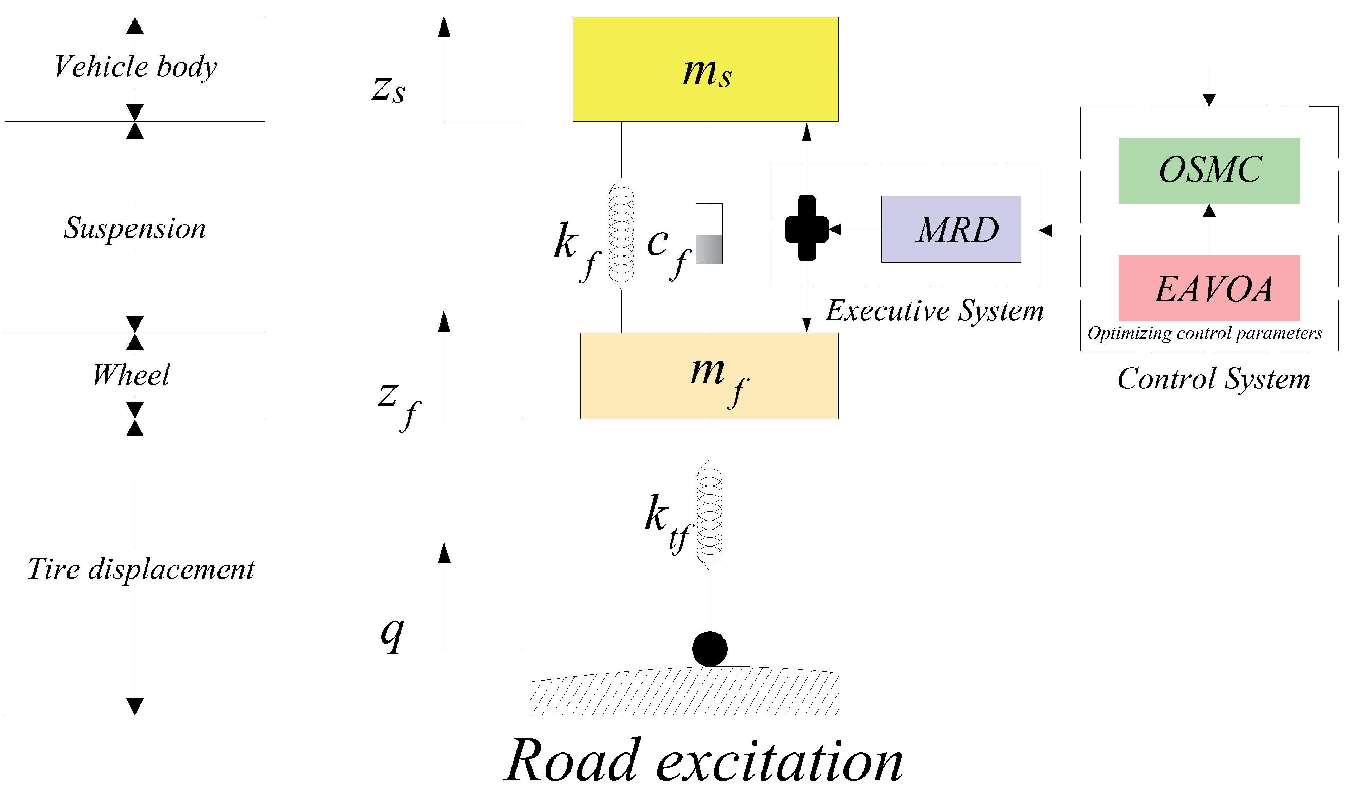
2.1. Mathematical Model of Automotive Suspension
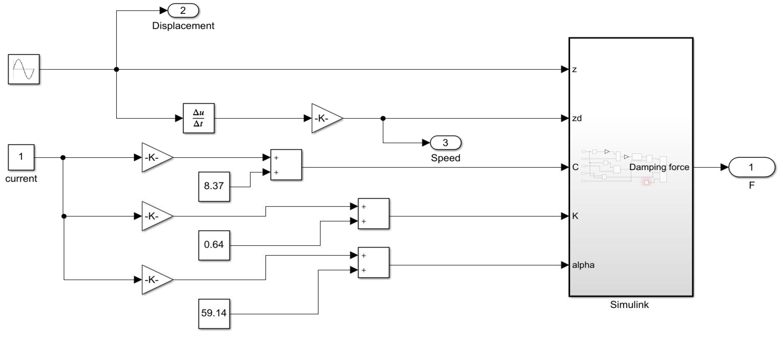
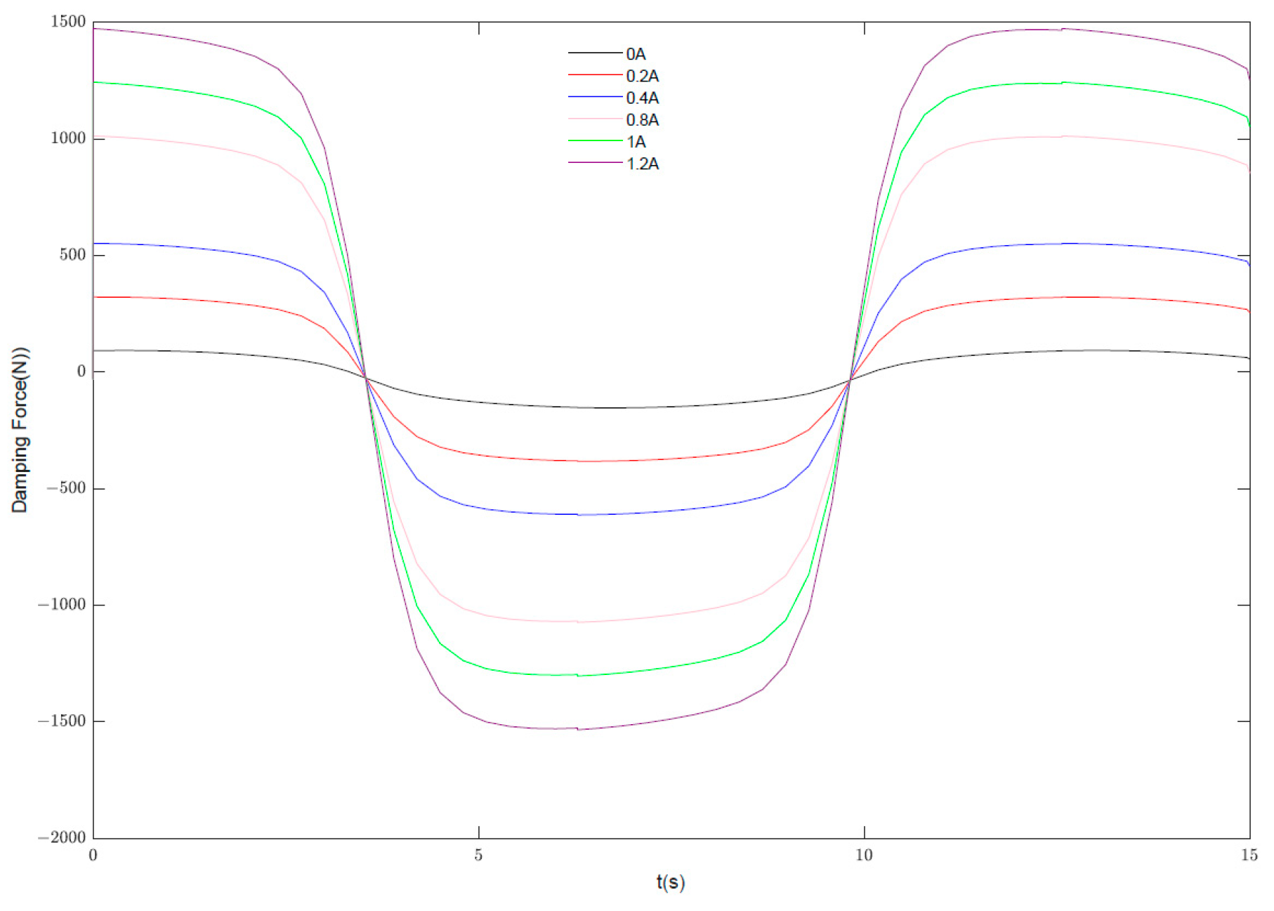
2.2. Automotive Suspension Actuator
3. Control Strategy
3.1. The Evaluation Criteria
3.2. The Design of OSMC
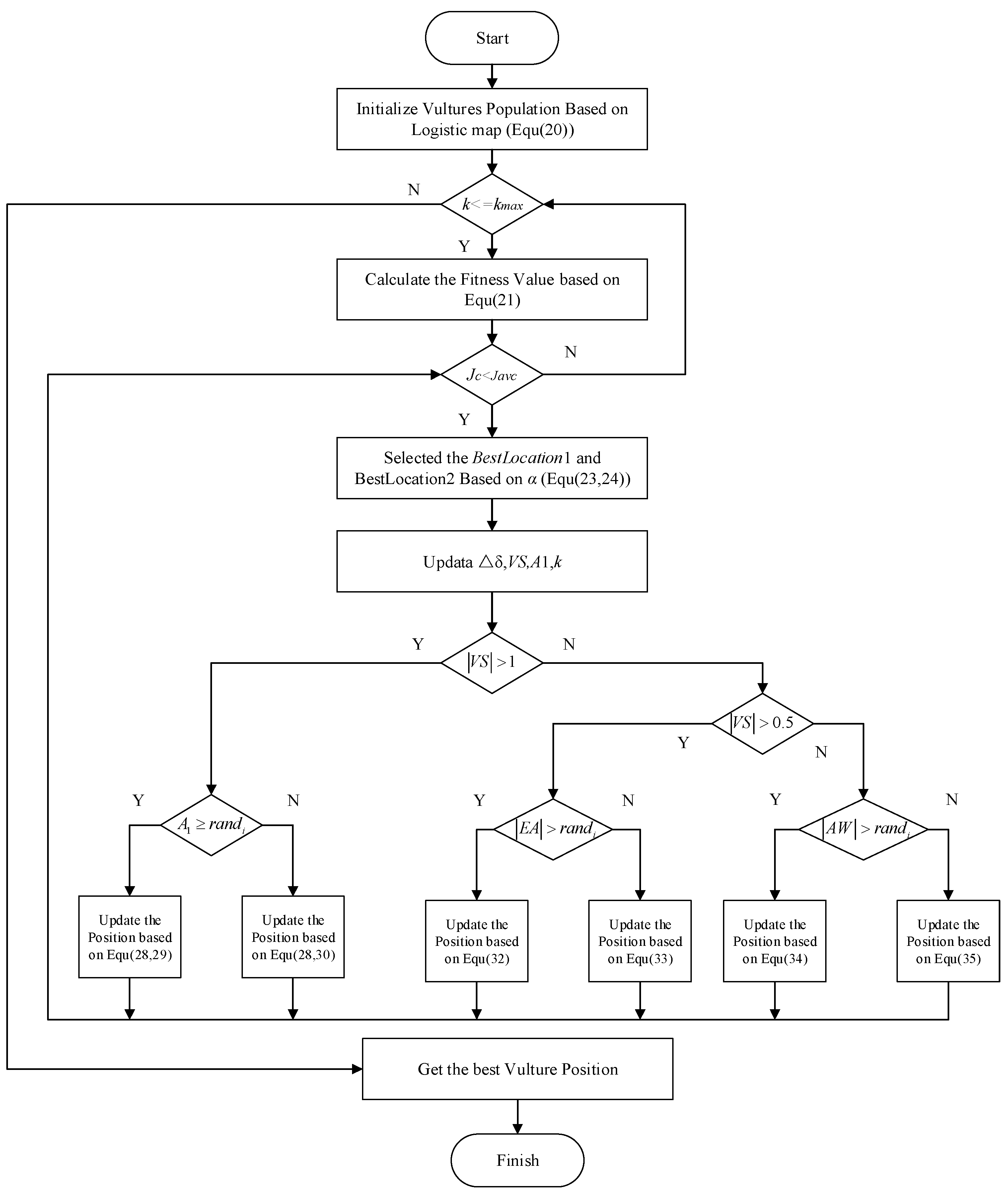
3.3. The Enhanced AVOA
- 1.
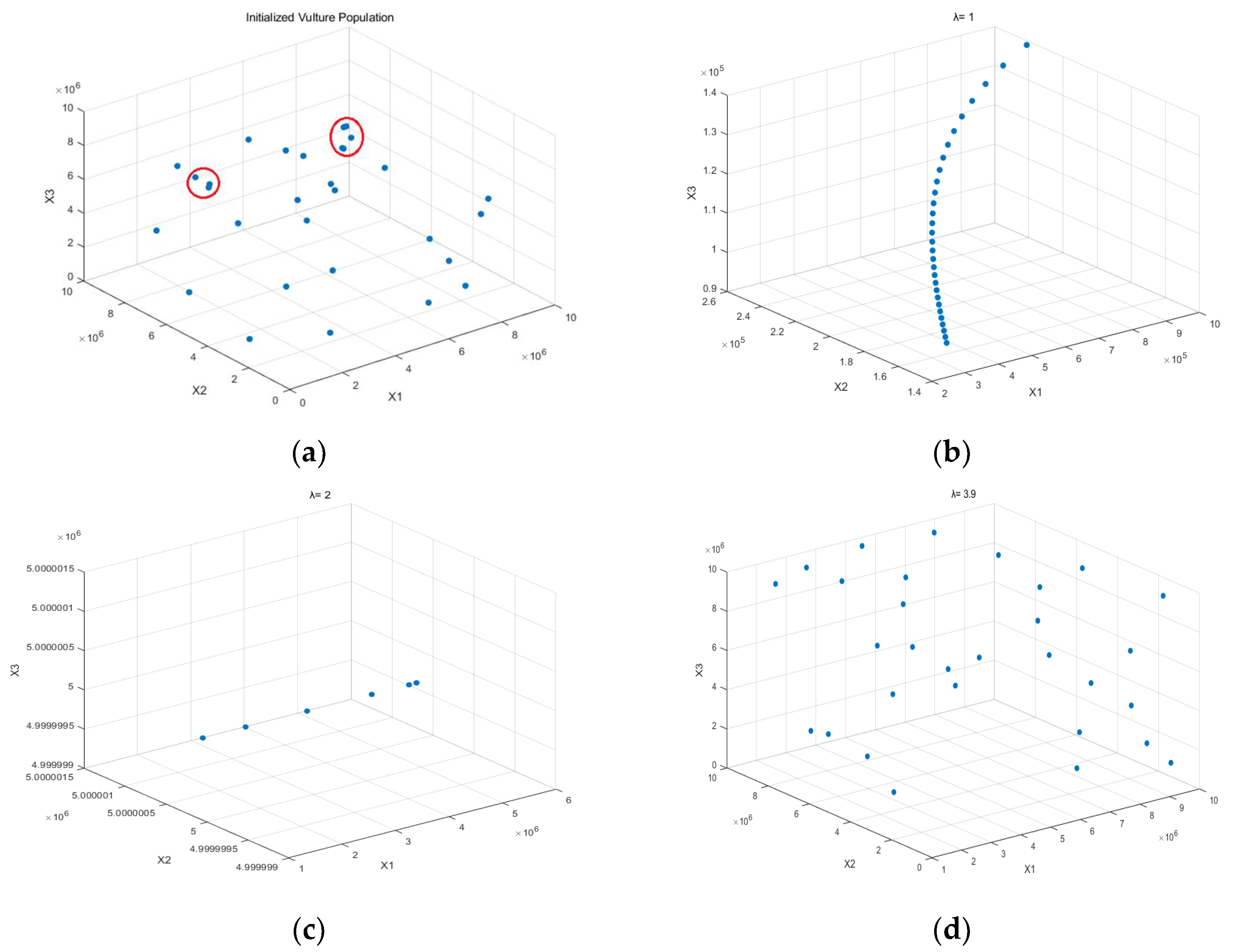
- To better initialize the population of vulture population, the Logistic map is adopted. The number of vulture populations is set to , and the dimension is set to . The expression of a single vulture and the Logistic map are as follows:
- 2.
- In the previous section, the suspension evaluation metric is established. When is smaller, it indicates a better suspension control performance. However, the is influenced by the units of these three-performance metrics and may not effectively balance these three performance aspects. As a result, the required fitness function will be obtained through Equation (21) in this paper.
- 3.
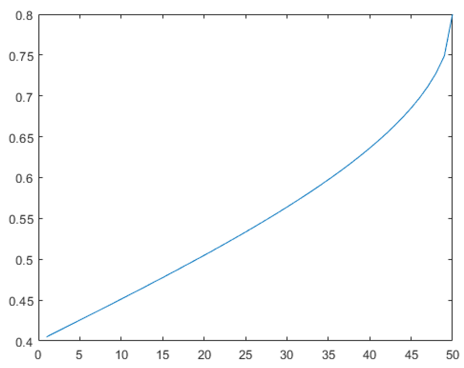
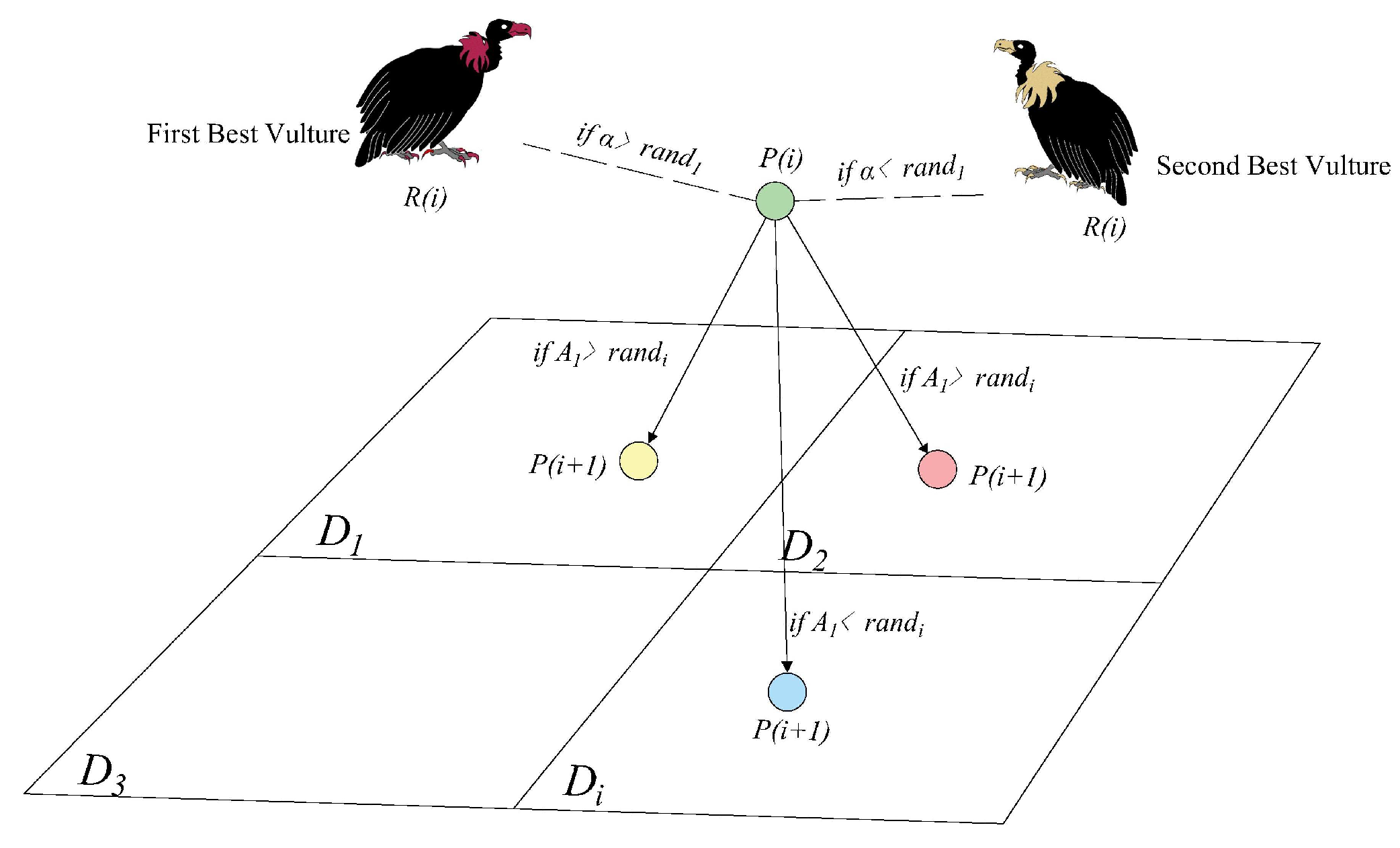
- After the vulture population is established and their respective fitness values are computed, the best solution is selected as the first group, embodying the optimal vulture value. The optimal solution for the second group is chosen as the second-best option. These two groups display two directions of vulture operation, and their formulae are as follows:where represents the current position. The value of is independent within the range . is the adjustment coefficient. In the AVOA, if the adjustment coefficient () is set to a fixed value, its value cannot be adjusted with iterations to enhance the search performance. When is a large value, it indicates a strong search capability. Where is a small value, it suggests the ability to conduct a broader search. To ensure the accuracy of the search, the extensive search is required and should be set to a smaller value in the initial stages. Once the search range is determined, the stronger search capabilities are needed and should be relatively large. Therefore, a nonlinear function is employed to optimize this value, and its formula is as follows:where represent the max and min values of the change interval and denotes the maximum number of iterations. The value of with iteration numbers is illustrated in Figure 6.
- 4.
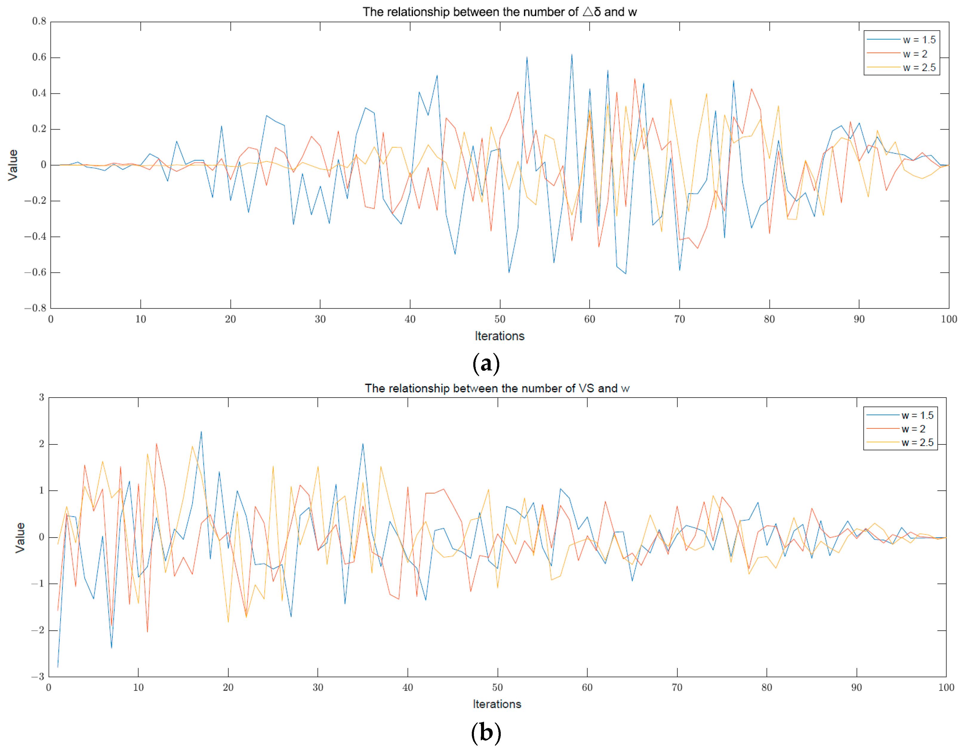
- The is introduced to represent the state of the vultures, with different levels of constraining the search range of these vultures. The is represented by Formula (27):where represents the perturbation value, displays the perturbation factor, is a random number within the range of [−2, 2], is a random number with the range of [−1, 1]. The is used to change the of the optimized vulture algorithm, so that it is not limited to a certain range and can fluctuate within a larger range. Different values of correspond to the varied search strategies. The perturbation value enhances the algorithm’s performance.
- 5.
- The is divided into three stages:
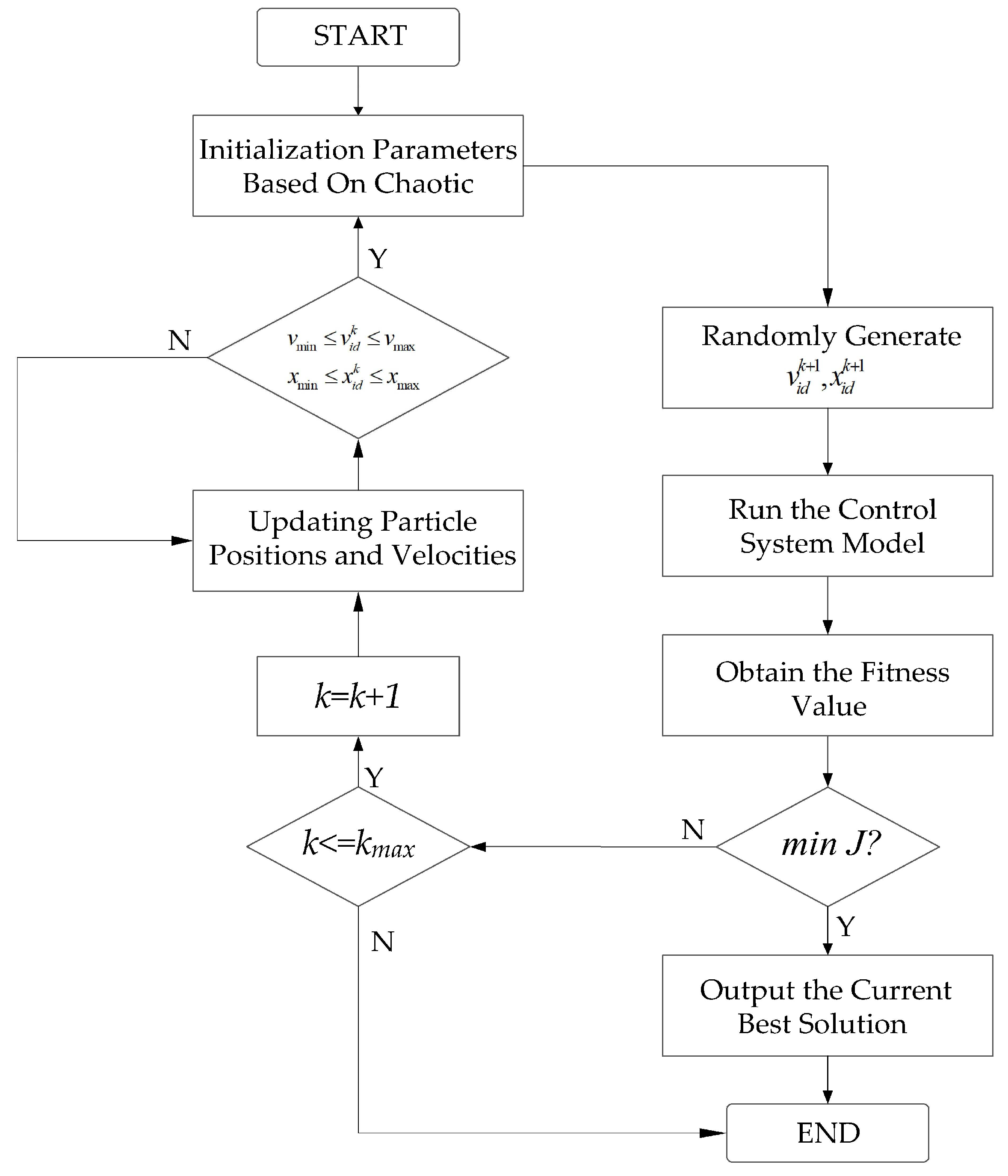
3.4. Optimizing OSMC Control Parameters Based on EAVOA
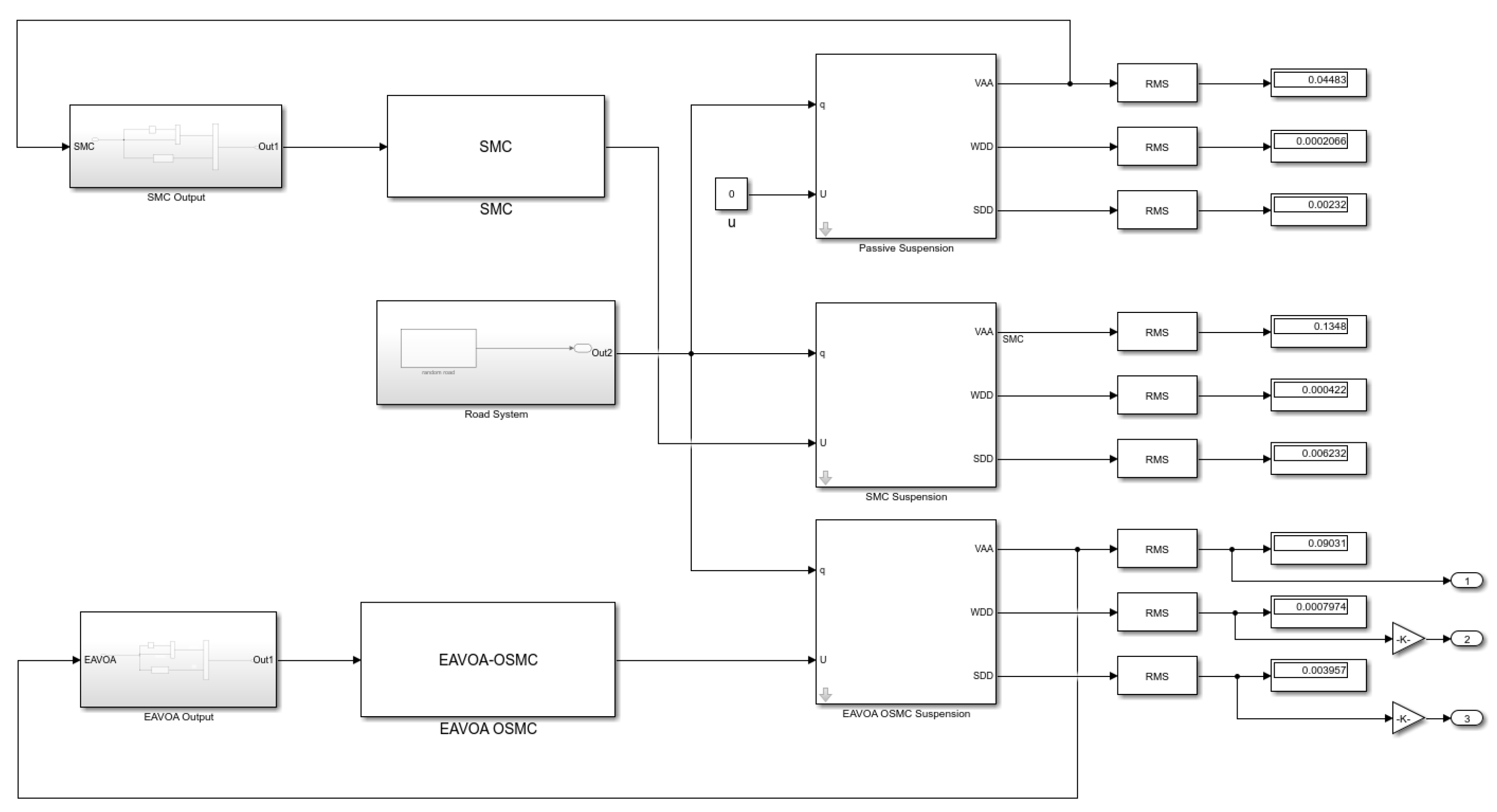
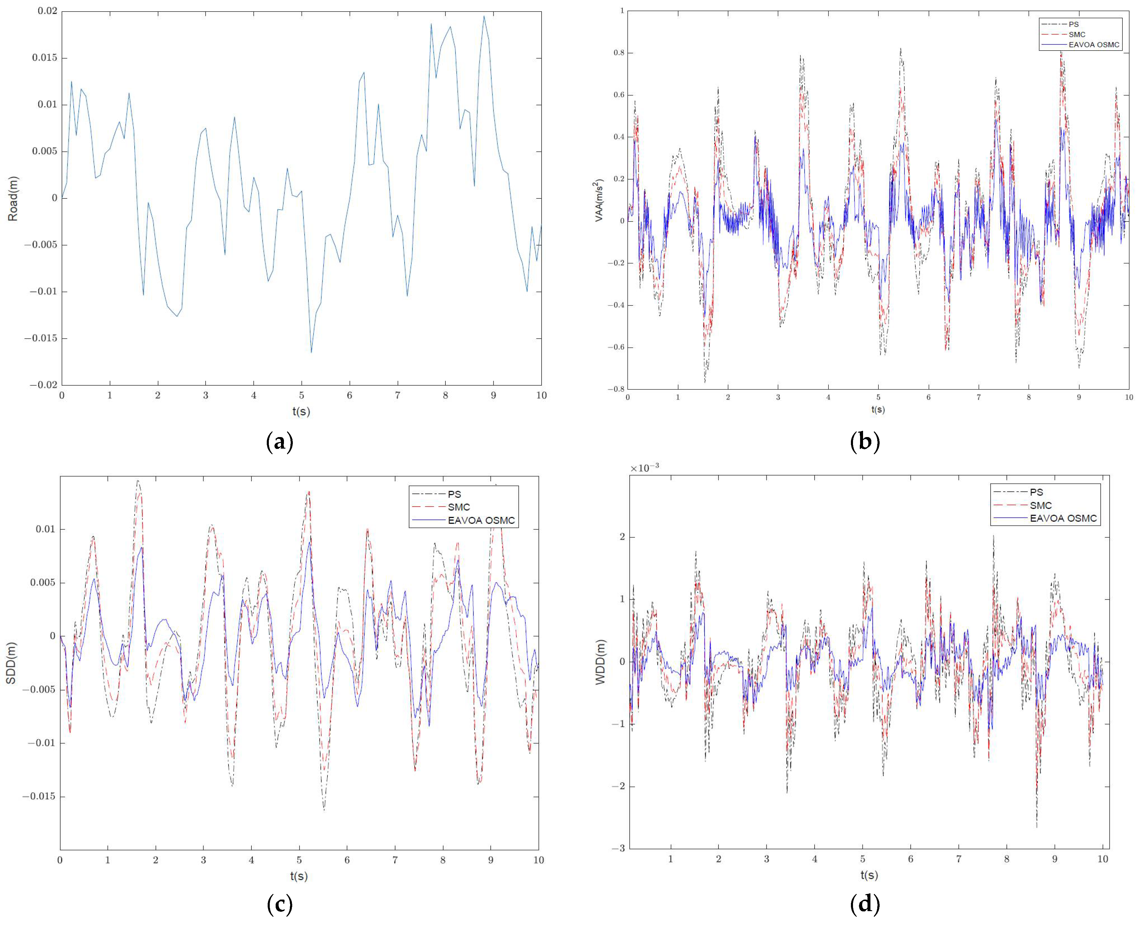
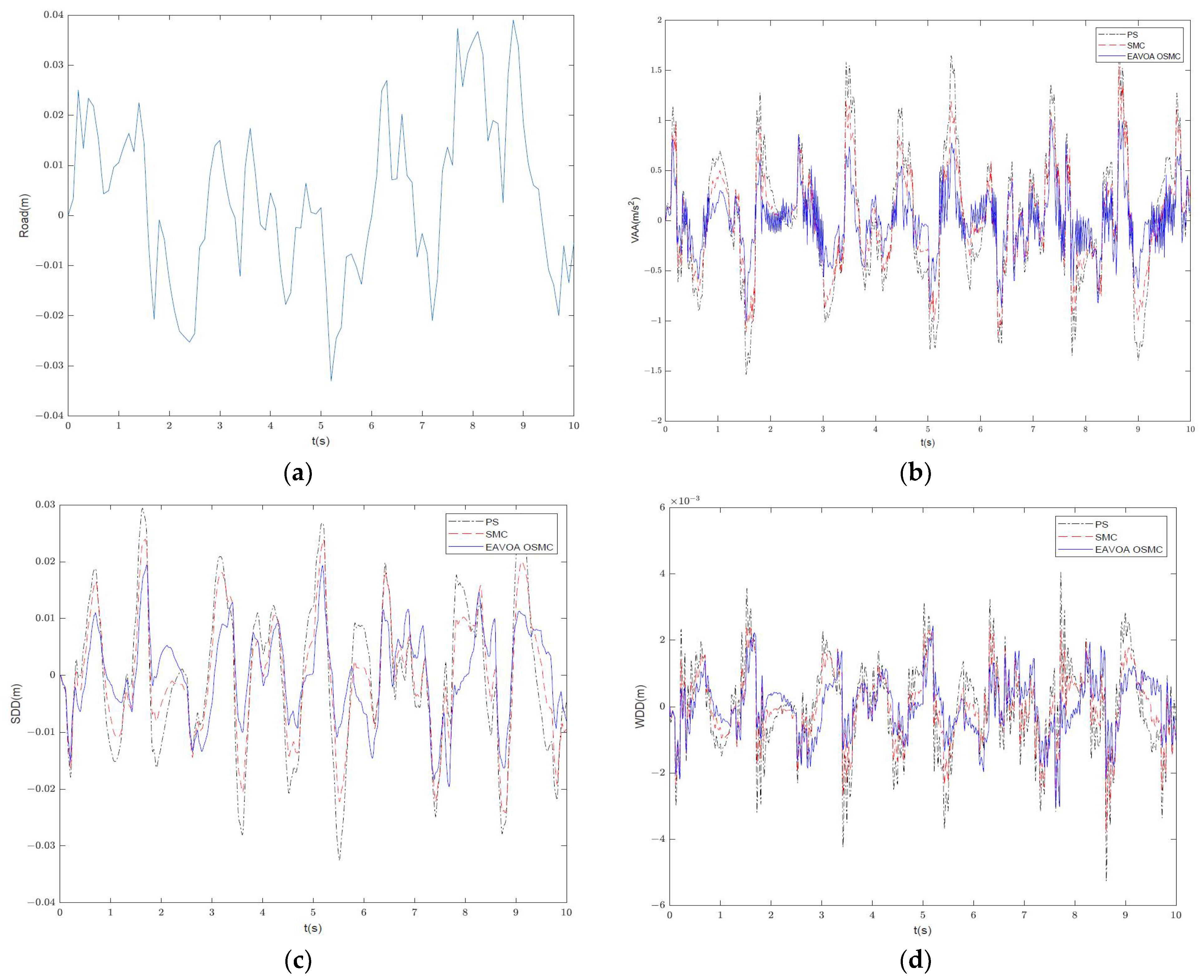
4. Simulation and Analysis
5. Discussion
- The combination of a semi-active suspension and an improved sliding mode control model to elucidate and determine the characteristics of SASS control strategy optimization.
- This paper utilizes chaotic mapping and nonlinear functions to improve the African vultures intelligent algorithm, which is then combined with a sliding mode controller to create an example for other scholars to study semi-active suspension comprehensive control strategies.
6. Conclusions
Author Contributions
Funding
Data Availability Statement
Conflicts of Interest
References
- Dižo, J.; Blatnický, M.; Gerlici, J.; Leitner, B.; Melnik, R.; Semenov, S.; Mikhailov, E.; Kostrzewski, M. Evaluation of Ride Comfort in a Railway Passenger Car Depending on a Change of Suspension Parameters. Sensors 2021, 21, 8138. [Google Scholar] [CrossRef] [PubMed]
- Miller, L.R. Tuning Passive, Semi-Active and Fully Active Suspension Systems. In Proceedings of the 27th IEEE Conference on Decision and Control, Austin, TX, USA, 7–9 December 1988; Volume 3, pp. 2047–2053. [Google Scholar]
- Yoshimura, T.; Kume, A.; Kurimoto, M.; Hino, J. Construction of an Active Suspension System of a Quarter Car Model Using the Concept of Sliding Mode Control. J. Sound Vib. J. Sound Vib. 2001, 239, 187–199. [Google Scholar] [CrossRef]
- Lin, J.; Lian, R.J. Intelligent Control of Active Suspension Systems. IEEE Trans. Ind. Electron. 2011, 58, 618–628. [Google Scholar] [CrossRef]
- Shiao, Y.; Lai, C.; Nguyen, Q. The analysis of a semi-active suspension system. In Proceedings of the SICE Annual Conference 2010, Taipei, Taiwan, 18–21 August 2010. [Google Scholar]
- Tran, G.Q.B.; Pham, T.-P.; Sename, O.; Costa, E.; Gaspar, P. Integrated Comfort-Adaptive Cruise and Semi-Active Suspension Control for an Autonomous Vehicle: An LPV Approach. Electronics 2021, 10, 813. [Google Scholar] [CrossRef]
- Wu, J.; Zhou, H.; Liu, Z.; Gu, M. Ride Comfort Optimization via Speed Planning and Preview Semi-Active Suspension Control for Autonomous Vehicles on Uneven Roads. IEEE Trans. Veh. Technol. 2020, 69, 8343–8355. [Google Scholar] [CrossRef]
- Yao, G.Z.; Yap, F.F.; Chen, G.; Li, W.H.; Yeo, S.H. MR damper and its application for semi-active control of vehicle suspension system. Mechatronics 2002, 12, 963–973. [Google Scholar] [CrossRef]
- Soliman, A.M.A.; Kaldas, M.M.S. Semi-active suspension systems from research to mass-market—A review. J. Low Freq. Noise Vib. Act. Control. 2019, 40, 1005–1023. [Google Scholar] [CrossRef]
- Tang, X.; Du, H.; Sun, S.; Ning, D.; Xing, Z.; Li, W. Takagi–Sugeno Fuzzy Control for Semi-Active Vehicle Suspension with a Magnetorheological Damper and Experimental Validation. IEEE/ASME Trans. Mechatron. 2017, 22, 291–300. [Google Scholar] [CrossRef]
- Alvarez-Sánchez, E. A Quarter-Car Suspension System: Car Body Mass Estimator and Sliding Mode Control. Procedia Technol. 2013, 7, 208–214. [Google Scholar] [CrossRef]
- Zhou, C.; Liu, X.; Chen, W.; Xu, F.; Cao, B. Optimal Sliding Mode Control for an Active Suspension System Based on a Genetic Algorithm. Algorithms 2018, 11, 205. [Google Scholar] [CrossRef]
- Ngoc, N.; Nguyen, T.A.; Duyen, D. A Novel Sliding Mode Control Algorithm for an Active Suspension System Considering with the Hydraulic Actuator. Lat. Am. J. Solids Struct. 2022, 19, e424. [Google Scholar] [CrossRef]
- Alves, U.N.L.T.; Garcia, J.P.F.; Teixeira, M.C.M.; Garcia, S.C.; Rodrigues, F.B. Sliding Mode Control for Active Suspension System with Data Acquisition Delay. Math. Probl. Eng. 2014, 1, 529293. [Google Scholar] [CrossRef]
- Pang, H.; Liu, F.; Xu, Z. Variable universe fuzzy control for vehicle semi-active suspension system with MR damper combining fuzzy neural network and particle swarm optimization. Neurocomputing 2018, 306, 130–140. [Google Scholar] [CrossRef]
- Wiseman, Y. Autonomous Vehicles, Encyclopedia of Information Science and Technology; IGI Global: Hershey, PA, USA, 2020. [Google Scholar]
- Basargan, H.; Mihály, A.; Gáspár, P.; Sename, O. Cloud-Based Adaptive Semi-Active Suspension Control for Improving Driving Comfort and Road Holding. IFAC-PapersOnLine 2022, 55, 89–94. [Google Scholar] [CrossRef]
- Brenner, N.; Jessop, B.; Jones, M.; Macleod, G. State/Space: A Reader; John Wiley & Sons: Hoboken, NJ, USA, 2008. [Google Scholar]
- Hamilton, J.D. State-Space Models. In Handbook of Econometrics; North-Holland: Amsterdam, The Netherlands, 1994; pp. 3039–3080. [Google Scholar]
- Chooi, W.W.; Oyadiji, S.O. Mathematical Modeling, Analysis, and Design of Magnetorheological (Mr) Dampers. J. Vib. Acoust. 2009, 131, 061002. [Google Scholar] [CrossRef]
- Brigadnov, I.A.; Dorfmann, A. Mathematical Modeling of Magnetorheological Fluids. Contin. Mech. Thermodyn. 2005, 17, 29–42. [Google Scholar] [CrossRef]
- Choi, S.; Lee, S.K.; Park, Y.P. A hysteresis model for the field-dependent damping force of a magnetorheological damper. J. Sound Vib. 2001, 245, 375–383. [Google Scholar] [CrossRef]
- Yu, W.; Zhu, K.; Yu, Y. Variable Universe Fuzzy PID Control for Active Suspension System with Combination of Chaotic Particle Swarm Optimization and Road Recognition. IEEE Access 2024, 12, 29113–29125. [Google Scholar] [CrossRef]
- Faraj, R.; Graczykowski, C.; Holnicki-Szulc, J. Adaptable Pneumatic Shock Absorber. J. Vib. Control. 2019, 3, 711–721. [Google Scholar] [CrossRef]
- Jeltsch, R.; Mansour, M. Stability Theory/Hurwitz Centenary Conference Centro Stefano Franscini, Ascona, 1995; Birkhäuser: Basel, Switzerland, 1996. [Google Scholar]
- Li, X.; Xu, N.; Guo, K.; Huang, Y. An Adaptive SMC Controller for EVs with Four IWMs Handling and Stability Enhancement Based on a Stability Index. Veh. Syst. Dyn. 2021, 59, 1509–1532. [Google Scholar] [CrossRef]
- Nasmyth, K.; Haering, C.H. The Structure and Function of SMC and Kleisin Complexes. Annu. Rev. Biochem. 2005, 74, 595–648. [Google Scholar] [CrossRef] [PubMed]
- Abdollahzadeh, B.; Gharehchopogh, F.S.; Mirjalili, S. African vultures optimization algorithm: A new nature-inspired metaheuristic algorithm for global optimization problems. Comput. Ind. Eng. 2021, 158, 107408. [Google Scholar] [CrossRef]
- Fan, J.; Li, Y.; Wang, T. An improved African vultures optimization algorithm based on tent chaotic mapping and time-varying mechanism. PLoS ONE 2021, 16, e0260725. [Google Scholar] [CrossRef]
- Gautestad, A.O.; Mysterud, I. Complex animal distribution and abundance from memory-dependent kinetics. Ecol. Complex. 2006, 3, 44–55. [Google Scholar] [CrossRef]
- Yang, X.S. Nature-Inspired Metaheuristic Algorithms, 2nd ed.; Luniver Press: Frome, UK, 2010. [Google Scholar]

| Value | w = 1.5 | w = 2 | w = 2.5 |
|---|---|---|---|
| 0.2549 | 0.1762 | 0.1539 | |
| 0.7528 | 0.7475 | 0.6319 |
| Symbol | Value | Unit | Symbol | Value | Unit |
|---|---|---|---|---|---|
| 330 | Kg | 2 | \ | ||
| 25 | Kg | −2 | \ | ||
| 13 | KN/m | 1 | \ | ||
| 170 | KN/m | 30 | \ | ||
| 1.2 | KN s/m | 0.01 | \ |
| Random Road Grade | Symbol | PS | SMC | EAVOA-OSMC |
|---|---|---|---|---|
| B | 0.32304 | 0.2606 | 0.1856 | |
| 0.0065 | 0.00593 | 0.00484 | ||
| 6.9528 × 10⁻⁴ | 5.6456 × 10⁻⁴ | 5.1281 × 10⁻⁴ | ||
| D | 0.6493 | 0.5245 | 0.4107 | |
| 0.0131 | 0.0105 | 0.0097 | ||
| 0.0014 | 0.0011 | 8.9723 × 10⁻⁴ |
| Random Road Grade | |||||
|---|---|---|---|---|---|
| B | 2.143 | −6.51 | 0.1306 | 0.562 | 28.14 |
| D | 3.527 | −8.33 | 0.1765 | 0.797 | 32.49 |
Disclaimer/Publisher’s Note: The statements, opinions and data contained in all publications are solely those of the individual author(s) and contributor(s) and not of MDPI and/or the editor(s). MDPI and/or the editor(s) disclaim responsibility for any injury to people or property resulting from any ideas, methods, instructions or products referred to in the content. |
© 2024 by the authors. Licensee MDPI, Basel, Switzerland. This article is an open access article distributed under the terms and conditions of the Creative Commons Attribution (CC BY) license (https://creativecommons.org/licenses/by/4.0/).
Share and Cite
Li, Y.; Fang, Z.; Zhu, K.; Yu, W. Sliding Mode Control for Semi-Active Suspension System Based on Enhanced African Vultures Optimization Algorithm. World Electr. Veh. J. 2024, 15, 380. https://doi.org/10.3390/wevj15080380
Li Y, Fang Z, Zhu K, Yu W. Sliding Mode Control for Semi-Active Suspension System Based on Enhanced African Vultures Optimization Algorithm. World Electric Vehicle Journal. 2024; 15(8):380. https://doi.org/10.3390/wevj15080380
Chicago/Turabian StyleLi, Yuyi, Zhe Fang, Kai Zhu, and Wangshui Yu. 2024. "Sliding Mode Control for Semi-Active Suspension System Based on Enhanced African Vultures Optimization Algorithm" World Electric Vehicle Journal 15, no. 8: 380. https://doi.org/10.3390/wevj15080380
APA StyleLi, Y., Fang, Z., Zhu, K., & Yu, W. (2024). Sliding Mode Control for Semi-Active Suspension System Based on Enhanced African Vultures Optimization Algorithm. World Electric Vehicle Journal, 15(8), 380. https://doi.org/10.3390/wevj15080380