Abstract
The sideslip angle and the yaw rate are the key state parameters for vehicle handling and stability control. To improve the accuracy of the input parameters and the time-varying characteristics of noise covariance in state estimation, a combined method of recursive least squares with a variable forgetting factor and adaptive iterative extended Kalman filtering is proposed for estimation. Based on the established three-degrees-of-freedom nonlinear model of the vehicle, the variable forgetting factor recursive least squares method is used to identify the tire cornering stiffness and serves as an input for vehicle state estimation. An innovative algorithm is used to optimise the uncertain noise covariance in the iterative extended Kalman filter (IEKF) process. Finally, with the help of the joint simulation of CarSim2019 and Matlab/Simulink R2022a, a distributed drive electric vehicle state parameter estimation model is established, and a simulation analysis of typical working conditions is carried out. Furthermore, an experiment is conducted with the pix moving vehicle and the integrated navigation system. The simulation and experimental results show that, compared to the traditional extended Kalman filter algorithm, the proposed algorithm improves the estimation accuracy of the yaw rate, sideslip angle, and longitudinal speed by 58.17%, 57.2%, and 76.47%, respectively, which shows that the algorithm has a higher estimation accuracy and a stronger applicability to provide accurate state information for vehicle handling and stability control.
1. Introduction
New energy vehicles are in the transition period from electrification to automation, a state in which the active safety system and intelligent assisted driving system are of great significance to the stability of vehicle operation. The sideslip angle is used as a handling dynamic state variable to characterise the vehicle’s performance in tracking a trajectory in coordination with the driver, while the yaw rate is used as a stability dynamic state variable to represent the stability of the vehicle’s motion state. A real-time accurate yaw rate, sideslip angle, and vehicle speed are the bases of vehicle stability control. The perfect stability control strategy applied to electric vehicles can decrease the driver’s operating difficulty and the risk of traffic accidents and improve the overall performance of the vehicle, especially in complex road conditions or adverse weather [1]. However, accurately obtaining these state parameters usually requires expensive inertial measurement units or photoelectric sensors, which are not practical for large-scale application in production vehicles. Recently, many studies have utilised algorithms combined with observational information from low-cost sensors to achieve the real-time and accurate estimation of vehicle state parameters [2]. Therefore, the accurate estimation of key vehicle state parameters is crucial for enhancing the vehicle’s handling stability, safety, and ride comfort. Additionally, vehicle state estimation technology is a crucial foundation for achieving advanced driver assistance systems, aiding autonomous driving systems in making accurate judgments and decisions in complex environments, thereby promoting the development of intelligent transportation.
There are two main methods for estimating vehicle motion state parameters. One is based on the physical model of the vehicle, and the other is from data-driven estimation. According to the different modelling principles, the estimation methods based on the vehicle model can be subdivided into estimation based on the kinematic model and estimation based on the dynamics model [3].
Federico Cheli et al. [4]’s method integrates the sideslip angle through a kinematic formulation, assuming that the longitudinal speed is known. This method takes less account of the effect of the cumulative integration error on the estimation accuracy, requires less accuracy of the vehicle model, has a certain robustness, and is less often used alone in practical processes [5]. Data-driven [6] vehicle state estimation methods do not rely on accurate physical models and vehicle parameters, and they utilise valid data from sensors, which are processed by deep learning or reinforcement learning algorithms to achieve the real-time estimation of a vehicle’s state. Srinivasan and others proposed a vehicle state estimation method based on an end-to-end recurrent neural network, which could achieve highly accurate speed estimation values with expensive external speed sensors [7]. Napolitano and others designed a two-network architecture based on FNN and RNN, where the first network was used to estimate longitudinal velocities, and the second network combined the longitudinal velocities to predict the sideslip angle [8]. The obtained results were in good agreement with the reference values. Although data-driven state estimation methods can quickly adapt to dynamically changing traffic environments, they have not been widely applied in engineering practice due to the limitation of requiring large amounts of historical data and real time.
The current dynamics estimation algorithms that are widely used in engineering practice are Kalman filter algorithms [9], which combine observations with estimation for conventional driving environments. Based on the Kalman filter, researchers have successively proposed a variety of improved filter algorithms: for instance, the PF (particle filter) reflects the changes in the posterior probability distribution of the state by changing the position of the particles and updating their weights, and many scholars have conducted research on state estimation based on the PF [10,11]. Chu Wenbo et al. [12] used unscented particle filtering to observe the vehicle motion state. Their algorithm can effectively avoid the problem of sampling data degradation, but it increases the computational complexity, which has a certain impact on the real-time requirements of the algorithm. Zhu et al. proposed an improved particle-filtering algorithm (MPF) for the higher accuracy estimation of key vehicle state parameters in an environment of sensor faults and excessive noise [13]. Although the PF is widely used for handling highly nonlinear problems, in vehicle state estimation, it is essential to minimise computational complexity to meet the real-time requirements and address the issue of particle degeneration.
Currently, the computationally simple EKF and UKF are relatively popular since the combined noise effects in vehicle state estimation approximate a Gaussian distribution. The UKF utilises the UT transform on top of the KF by selecting a specific sigma point to convert it nonlinearly. Zhang Yixi et al. [14] used an ant-lion optimisation algorithm to optimise the noise covariance matrix in the UKF and to accurately estimate the sideslip angle and the yaw rate of the vehicle’s traverse. The EKF is based on the principle of the KF to perform Taylor expansion of a nonlinear system at a specific point and linearise the nonlinear system by solving the Jacobian matrix. Gang Li et al. [15] optimised the noise covariance matrix of the EKF with the Sage-Husa algorithm for the real-time estimation of a vehicle’s state. Wang et al. [16] considered the effect of sensor data loss and proposed a new adaptive fault-tolerant extended Kalman filter to improve the observer’s immunity to interference. Li proposed an adaptive EKF algorithm, which treats the change in the sideslip angle as feedback to compensate for the model error and adds a damping term to improve the accuracy [17]. However, these algorithms fail to adequately account for the effect of stage errors induced by the EKF when performing the Taylor expansion. Since the UKF needs to ensure the positive characterisation of the noise covariance matrix for each transformation, the EKF is chosen as the basic algorithm for the study, and the stage error of the EKF is reduced through an iterative process.
This study proposes a vehicle state estimation method based on the fusion of VFFRLS and AIEKF. Conventional research methods are based on accurate tire cornering stiffness and noise covariance matrices. However, parameter changes could degrade the accuracy or even make the filter diverge. Therefore, this study first uses the recursive least squares method with a variable forgetting factor (VFFRLS) to identify the tire cornering stiffness, and the iterative extended Kalman filter (IEKF) is used as the basic algorithm for vehicle state estimation. The method reduces the stage error and improves the accuracy compared to the EKF. At the same time, the algorithm employs an innovative algorithm to optimise the uncertain noise covariance of the process. Finally, the stability and accuracy of the algorithm are verified by co-simulation and experiment.
2. Vehicle Dynamic Model
2.1. Nonlinear Vehicle Three-Degrees-of-Freedom Model
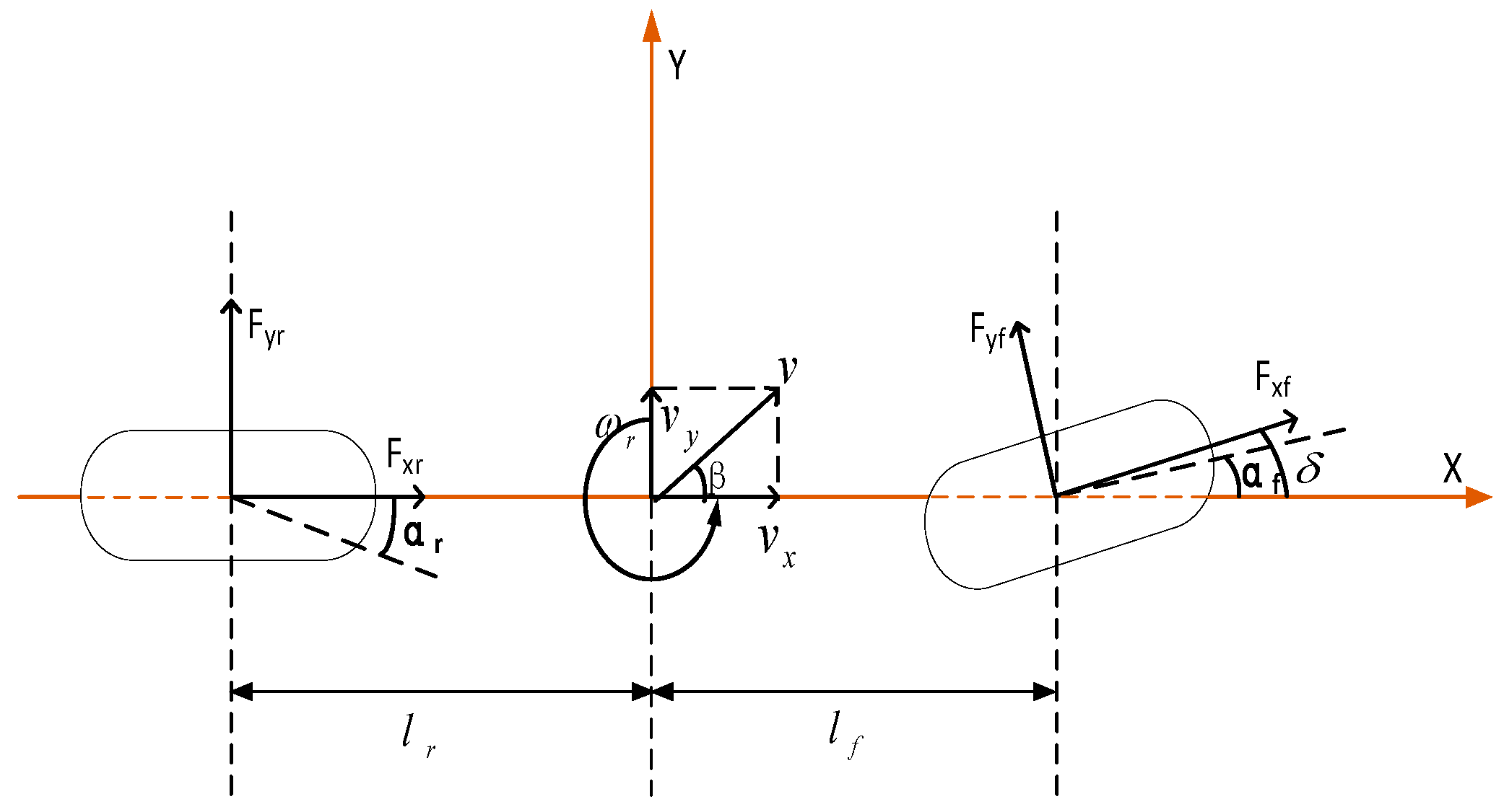
As shown in Figure 1, a nonlinear three-degrees-of-freedom vehicle model includes longitudinal, lateral, and yaw motions.
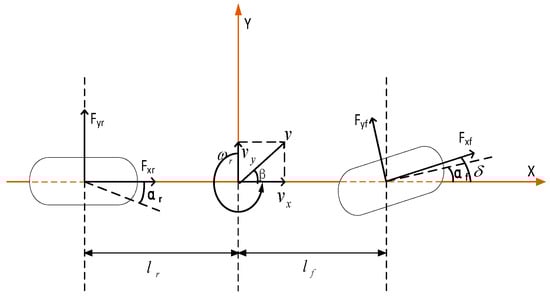
Figure 1.
Single-track three-degrees-of-freedom vehicle model.
The equation of longitudinal motion is
The equation of lateral motion is
The equation of yaw motion is
where is the mass of the vehicle; and are the longitudinal and lateral accelerations, respectively; and are the longitudinal and lateral forces of the wheels, respectively; denote the left front wheel, right front wheel, left rear wheel, and right rear wheel, respectively; is the moment of inertia of the vehicle about the Z axis; is the steering angle of the front wheel; and are the distance between the centre of gravity and the front axle and rear axle, respectively.
According to the vehicle’s dynamic equations, the state equations and measurement equations for the three-degrees-of-freedom vehicle are derived as follows
where is the yaw rate; is the sideslip angle; and are the cornering stiffnesses of the front axle and rear axle, respectively; is the longitudinal speed; is the lateral speed; and are longitudinal acceleration and lateral acceleration of the vehicle, respectively; is the moment of inertia of the vehicle about the Z axis.
2.2. Tire Model
The vehicle tire is in direct contact with the ground, supporting the vehicle’s weight, transmitting driving and braking torque and playing a crucial role in the vehicle’s safe operation [18]. The forces (lateral force, longitudinal force, vertical force) between the tire and the ground determine the actual motion of the vehicle. However, the tire structure is complex, and the nonlinear characteristics gradually increase with an increase in the side deflection angle; the accuracy of the tire model has a particular impact on the stability of vehicle handling. Therefore, a reliable tire model is necessary to estimate vehicle states accurately. The more commonly used tire model in vehicle dynamics is the magic tire model proposed by Professor H.B. Pacejka [19]. As a semi-empirical model, its expression is simple and has the nonlinear characteristics of tires with high fitting accuracy. The magic tire model expression is given as follows
where is the tire longitudinal force, lateral force, or aligning torque; depending on could represent the longitudinal slip rate or sideslip angle of the tire; is the peak factor; is the shape factor of a curve; is the curvature factor of a curve; is the stiffness factor; is the vertical offset; is the horizontal offset.
In observing vehicle state parameters, the longitudinal slip rate and the longitudinal and lateral tire forces could be given as follows
where is the longitudinal slip rate of each tire; is the tire radius; is the sideslip angle of each tire (from Equations (11) and (12)); the values of parameters , , , and can be calculated using the formulas provided in reference [20], which include the vertical load, roll angle, and fitting parameters. The fitting parameters to have already been determined through tire testing in reference [20].
3. Vehicle State Estimation Based on VFFRLS and AIEKF
3.1. Tire Cornering Stiffness Estimation Based on VFFRLS
For nonlinear vehicle systems, the tire cornering stiffness is an important parameter for linearising the vehicle model and a prerequisite for vehicle state parameter identification. Its realisation of accurate estimation is significant for vehicle manoeuvring stability. To avoid the correction term gradually decreasing to zero with an increase in sampling data and the phenomenon of false data saturation caused by the increasingly weak correction ability, this study introduces the concept of the variable forgetting factor. The forgetting factor is dynamically adjusted according to the real-time estimation error to improve the speed and robustness of the algorithm. This section uses the recursive least squares method with a variable forgetting factor to identify the tire cornering stiffness [21].
The fundamental vector equation for the least squares method is
where is the output vector; is based on the data vector provided by the sensor; is the unknown vector to be estimated; is the vector of the noise matrix.
When the tire side slip angle is small, the front and rear tire side slip angles are expressed as follows
where and are the front axle side slip angle and rear axle side slip angle, respectively; is the yaw rate of the vehicle.
The tire cornering force equation is transformed into the least squares form as follows
where is the tire cornering stiffness; is the tire side slip angle; = 1, 2 represents the front and rear axles, respectively; is the observation noise and model error during the tire cornering stiffness estimation.
The principle of recursive least squares with a forgetting factor is to determine an estimate , which minimises the sum of squared errors between the actual and estimated values and the objective function within the window of historical data under study. The objective function is defined as follows
where is a diagonal matrix consisting of forgetting factors.
The variable forgetting factor recursive least squares formula is derived as follows
Then, the recursive equation combining the tire cornering stiffness estimates is as follows
where the gain coefficient of parameter identification is recursively formulated as
The error covariance matrix is updated with the equation as follows
where is the estimated value of the tire cornering stiffness at the moment ; is a variable forgetting factor.
The gain and covariance matrix are only affected by the initial values and sensor signals. This results in the optimal forgetting factor at each time step.
The error between the estimated and actual values of the model at moment is as follows
The smaller means more trust in the new data, and the larger means more trust in the old data. To guarantee that the current moment and the overall trend are optimal, a variable forgetting factor function is established analogously to the loss function in neural networks as follows
where and are the moderating range of the forgetting factor. The forgetting factor of recursive least squares is considered to be between 0.95 and 1. Therefore, the value of is 1, and the value of is 0.95, is a positively adjustable parameter. In order to keep the value of the forgetting factor within the adjustment range, the value of is 5 [22].
3.2. Iterative Extended Kalman Filter Algorithm
The EKF (extended Kalman filter) is selected as the primary vehicle state estimation algorithm. The EKF algorithm is relatively simple to implement and has a certain robustness to the model uncertainty. The IEKF algorithm is employed to correct the truncation error caused by the first-order Taylor expansion in the EKF algorithm. The linearisation point is set to the a posteriori value of the last iteration in each iteration until the error of two consecutive iterations is less than the set value or the maximum number of iterations is reached, effectively improving the algorithm’s accuracy. The noise in vehicle state estimation includes the superposition of several independent noises, such as sensor errors, environmental perturbations, modelling errors, etc. The combined effect of these independent noises based on the Central Limit Theorem allows the total noise to be approximated as a Gaussian distribution.
The iterative extended Kalman filter is an iterative recursive filter that requires the discretisation of continuous-time systems, and the state space expression obtained by discretising Equations (4) and (5) using the forward Euler method is given by
where and denote the state equation function and observation equation function, respectively; represents the state vector; represents the input vector, which can be obtained from the longitudinal acceleration sensor and steering angle sensor at low cost; represents the observation vector; is the Gaussian white noise of the system process with covariance matrix ; is the Gaussian white noise of the observation process with covariance matrix .
The Jacobi matrices’, and , computation completes the linearisation of the nonlinear equations of state and observation. The equation of state function and the observation equation function of the vehicle nonlinearity are partial derivatives of the state at time to obtain the Jacobi matrices and , respectively.
After the linearisation is completed, initial values are assigned to the three state variables and covariance matrix to be estimated, followed by the IEKF algorithm process as follows
The prediction step is
The update step is
where is the error covariance matrix of the prediction step; is the Kalman gain; is the innovation vector; and is the number of iterations.
3.3. AIEKF Algorithm
The adaptive estimation algorithm based on innovation is less dependent on previous statistical information, some weight is given to the accuracy of the previous information, and the new observation and process noise covariance matrices are adapted according to the iterative results of the filter learning history [23]. The adaptive estimation algorithm based on innovation is used to adjust the noise covariance matrix of the estimation process [24]. The algorithm improves the robustness and adaptability of the estimation of the IEKF algorithm. Since simultaneously compensating and could lead to filter divergence, the compensated process noise covariance matrix is robust. Therefore, the adaptive iterative extended Kalman Filter (AIEKF) observer is updated with only the R matrix. In addition, the computation of is also feasible for other problems.
The method uses a sliding window of length N for the mean of the previous residual series. When the number of iterations is greater than or equal to N, the estimated covariance matrix of the innovation is given by
Considering the trade-off between estimation performance and computational burden, the sliding window length N in AIEKF is chosen as 16, and is the innovation vector in the IEKF algorithm. From this, the innovation update formula for the observation noise covariance can be derived as
where the equation for the change in state is
When the system reaches a steady state, the observation noise covariance is updated with the equation.
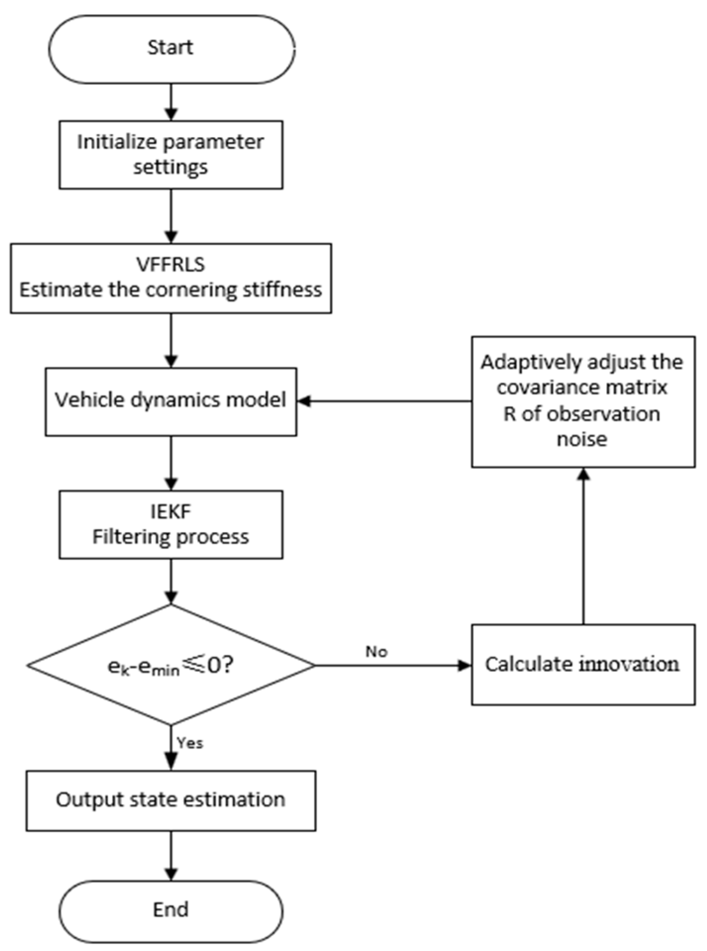
Therefore, a flowchart of the VFFRLS-AIEKF state estimation algorithm is shown in Figure 2.

Figure 2.
VFFRLS-AIEKF algorithm flowchart.
4. Simulation and Experiment Results
Co-simulation with CarSim2019 and Simulink R2022a verifies the accuracy of the proposed algorithm. A certain D-class car in CarSim2019 is selected for the simulation vehicle, and the parameters are shown in Table 1.

Table 1.
Vehicle parameter settings.
4.1. Tire Cornering Stiffness Estimation
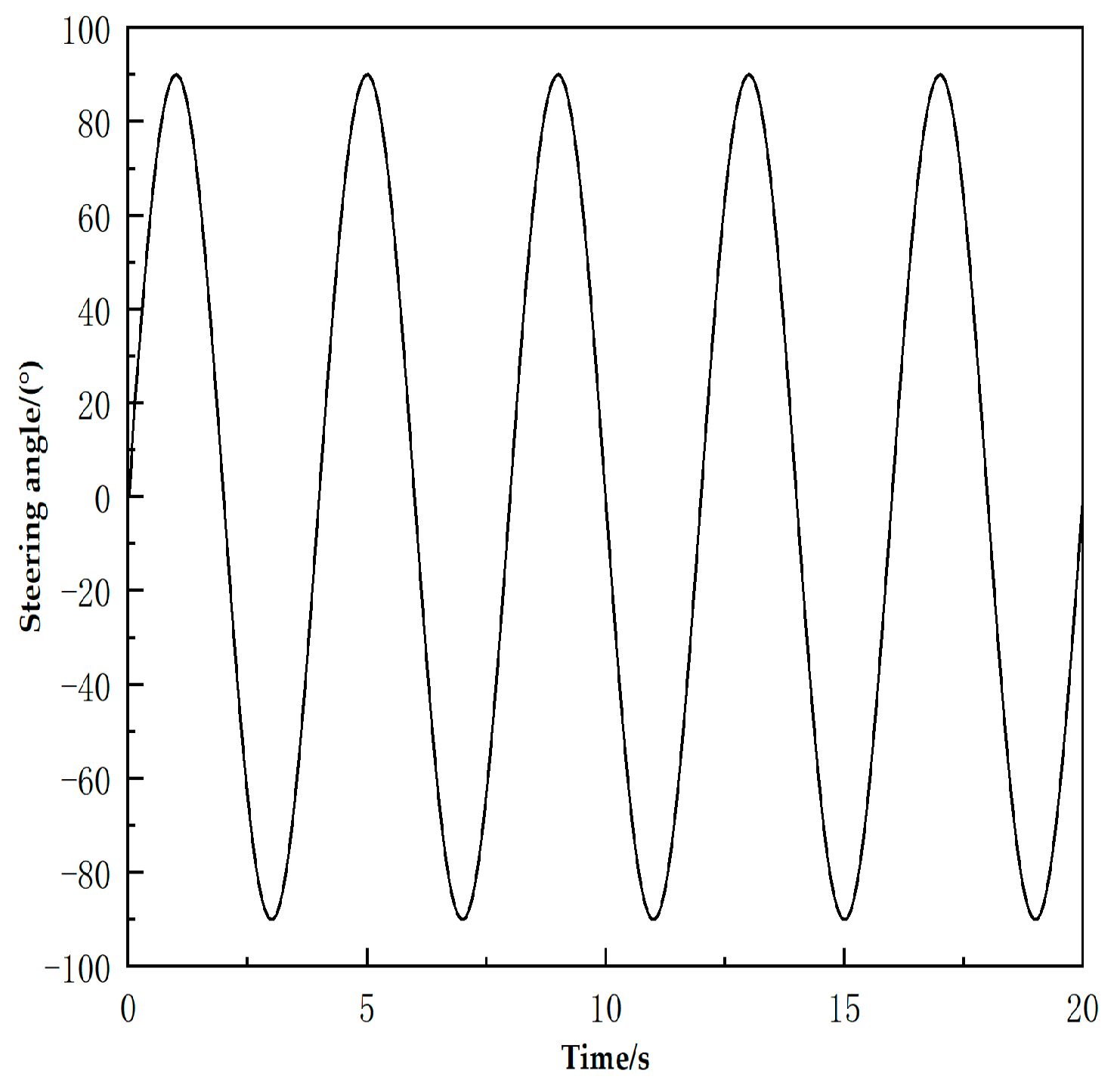
The steering wheel angle is a sinusoidal input (90°, 0.25 Hz), the road adhesion coefficient is set to 0.85, the speed is 60 km/h, and the sampling frequency is 1000 Hz.
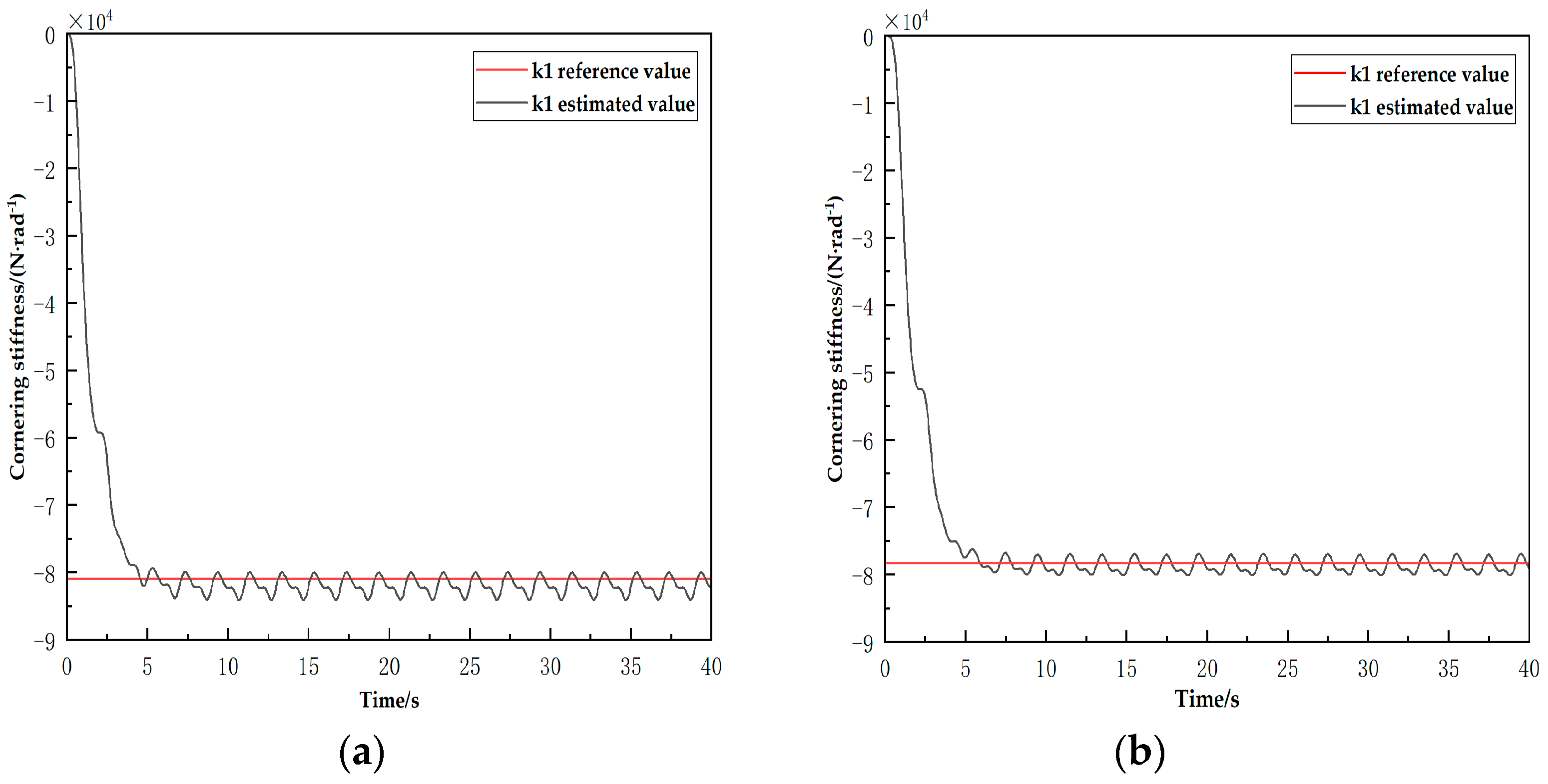
The side slip angles of the front and rear wheels in CarSim2019 are less than 4 degrees, and the cornering force is linearly related to the side slip angle. So, the ratio of the maximum cornering force to the maximum side slip angle of the front and rear wheels from CarSim2019 is selected as the reference value for estimating the cornering stiffness. As shown in Figure 3 and Figure 4, the cornering stiffness of the front and rear wheels estimated by the recursive least squares method based on the variable forgetting factor keeps fluctuating around the constant reference value near the 5 s period, and the convergence speed is faster. Meanwhile, the maximum relative error between the estimated cornering stiffness of the front wheel and the reference value after 5 s is 1.22%, and the maximum relative error between the estimated cornering stiffness of the rear wheel and the reference value is 1.21%. The relative error of this method meets the control requirements. Therefore, this algorithm has a fast convergence speed and high estimation accuracy. When the cornering force and side slip angle cannot be observed precisely, the tire cornering stiffness is determined by this algorithm to obtain a better control effect, and it is used as an important input for state observation.
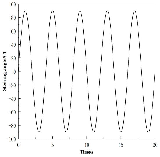
Figure 3.
Steering-angle variation under the sinusoidal steering condition.
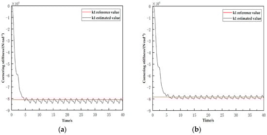
Figure 4.
Simulation results of tire cornering stiffness: (a) simulation result of front tire cornering stiffness; (b) simulation result of rear tire cornering stiffness.
4.2. Validation of the AIEKF Algorithm
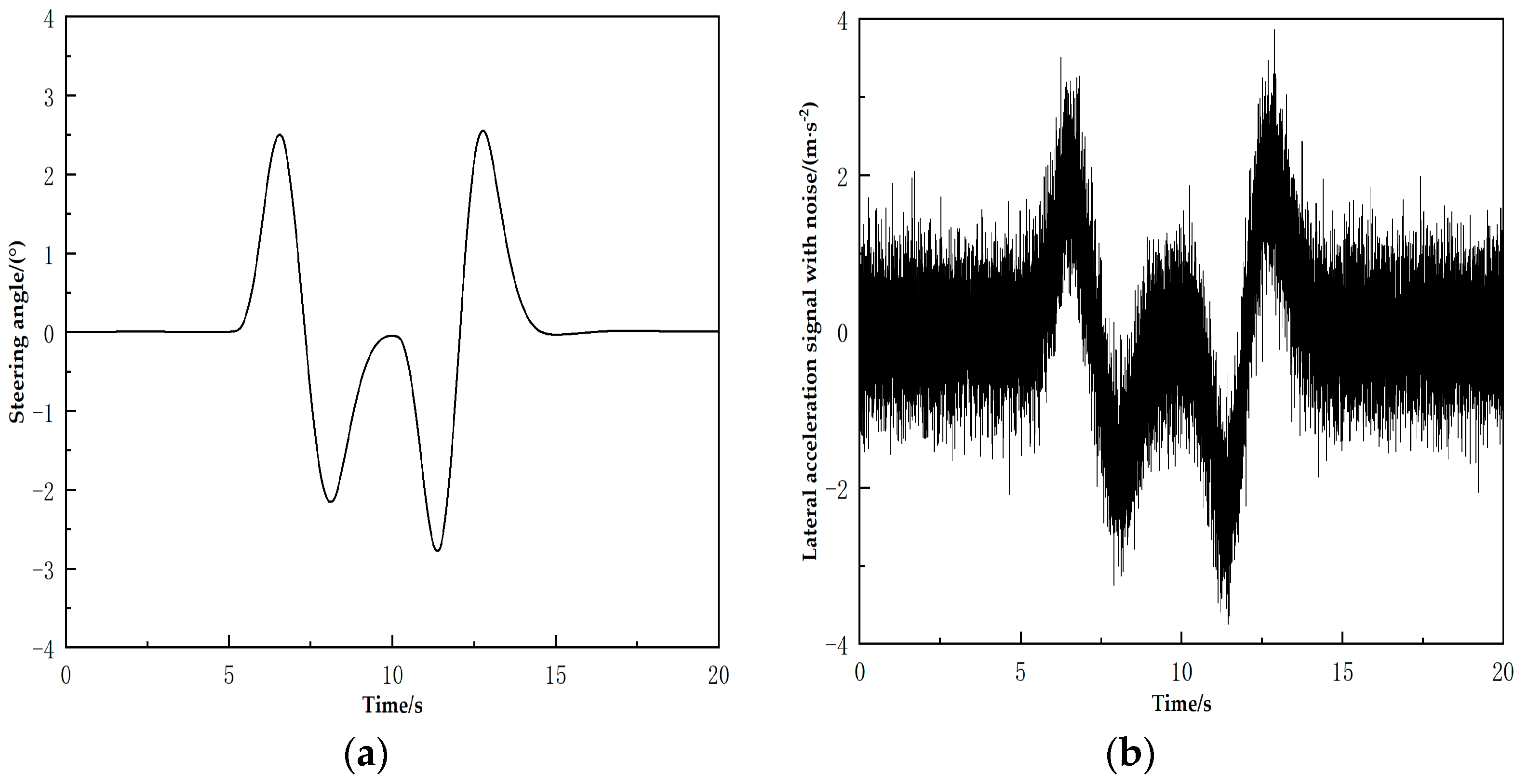
The typical condition of double-lane change is usually used to evaluate the manoeuvring stability of the vehicle under different road conditions. The input is the double-lane-change condition in CarSim2019, with a 40 km/h speed. The initial value of the system state vector is set to . The front wheel angle and lateral acceleration with Gaussian white noise are shown in Figure 5. The value of the road adhesion coefficient is set to 0.85, and the sampling frequency is 1000 Hz.
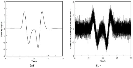
Figure 5.
Steering angle and noise change curve: (a) steering-angle variation under the double-lane-change condition, reprinted from Ref. [25]; (b) observation signal with time-varying Gaussian white noise.
The tire cornering stiffness estimated by the recursive least squares method with a variable forgetting factor is used as the input to the vehicle state observer. The simulation results of the AIEKF algorithm, compared with the reference values output by CarSim2019 and the estimation results of the EKF algorithm, are shown in the figure below. The initialisation parameters of the AIEKF algorithm for the whole state estimation are set. The initial value of the error covariance matrix is set to eye (3) 0.1, the initial value of the system process noise covariance matrix is set to eye (3), and the initial value of the observation noise covariance matrix is set to 10,000.
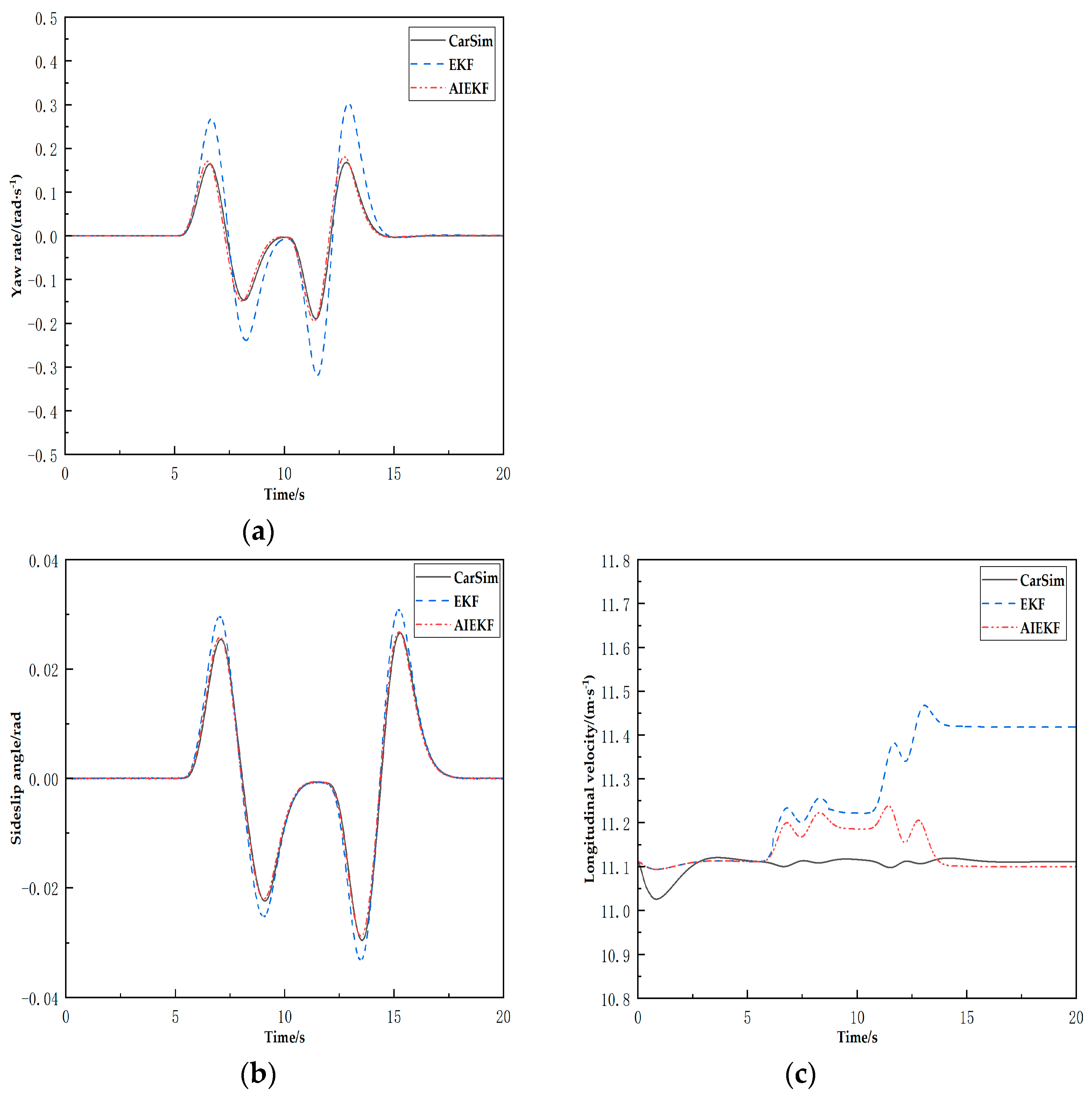
The simulation results show that the accuracy of the proposed AIEKF estimation algorithm is significantly higher than that of the EKF algorithm. As shown in Figure 6, the vehicle is traveling in the 5 s–15 s interval of lane changing under the double-lane-change condition. When the steering wheel angle responds rapidly, the sideslip angle and the yaw rate from the EKF algorithm will deviate from the ideal value, in which the yaw rate is more pronounced, and the proposed AIEKF algorithm could track the ideal value more accurately. At the same time, when the yaw rate and the sideslip angle reach the threshold value, the EKF algorithm estimates less accurately, and the AIEKF is still able to estimate accurately in this case, which is less affected by the fluctuation. As shown in Figure 6, the longitudinal speed from the EKF algorithm is greatly affected by the noise covariance during the vehicle changing lanes. It deviates from the target value, the maximum relative error is 5.35%, and there is a steady-state error after 14.2 s. Because the longitudinal speed estimated by the proposed AIEKF algorithm is adaptively updated, the accuracy is greatly improved, and the maximum relative error is 1.27%, which can satisfy the requirement of control accuracy.
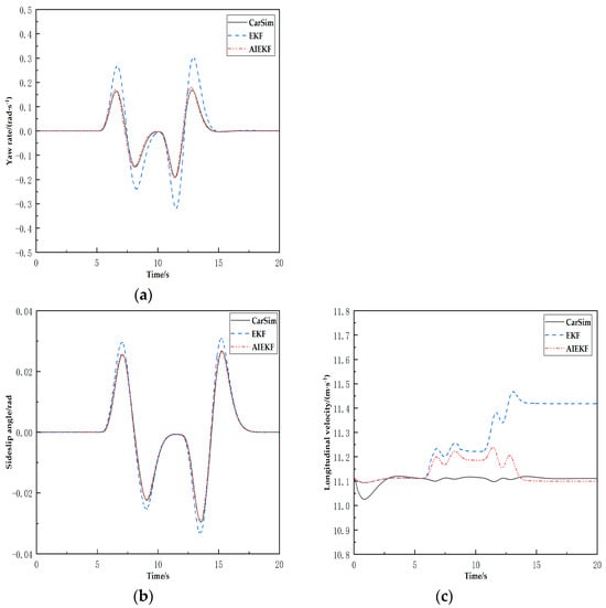
Figure 6.
Simulation results of vehicle state estimation: (a) variation result of yaw rate; (b) variation result of sideslip angle; (c) variation result of longitudinal velocity.
4.3. Experimental Validation
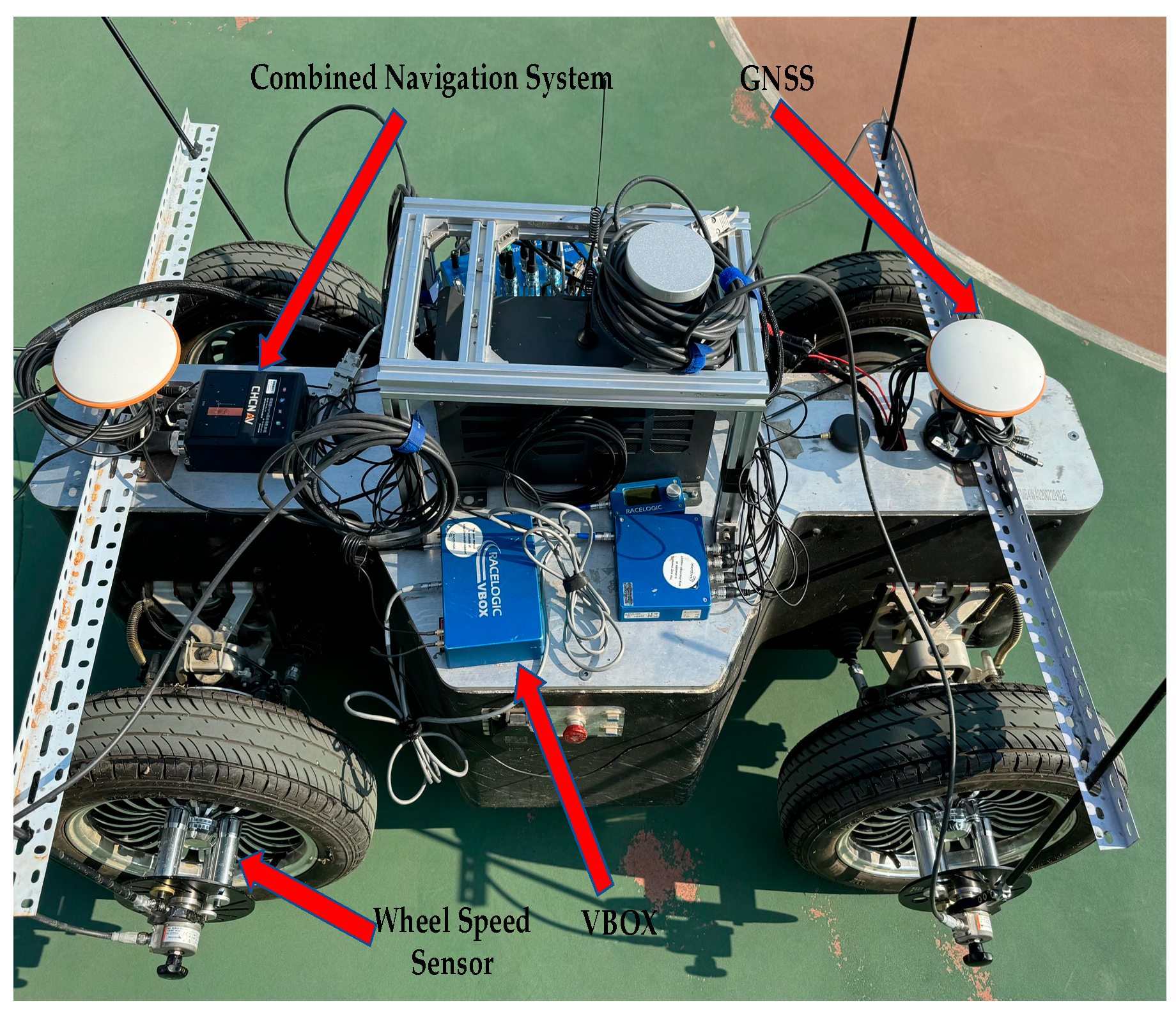
To further validate the accuracy of the proposed vehicle state estimation, a pix moving four-wheel-hub motor vehicle is applied to the experiment. As shown in Figure 7, a VBOX and four KISTLER wheel speed sensors measure the speed of the vehicle and wheels, respectively. The experiment uses the CGI-410 centimetre-level combined navigation system to obtain real-time longitudinal and lateral acceleration signals, yaw rate, and sideslip angle signals from the vehicle. The integrated navigation system incorporates high-precision MEMS gyroscopes and accelerometers, utilizing a combination of INS and GNSS navigation technology to obtain high-precision sensor information [26]. The test process requires logging into the RTK client to obtain differential data. The collected GPCHC data are analysed using serial debugging tools and the corresponding protocols to receive text data.
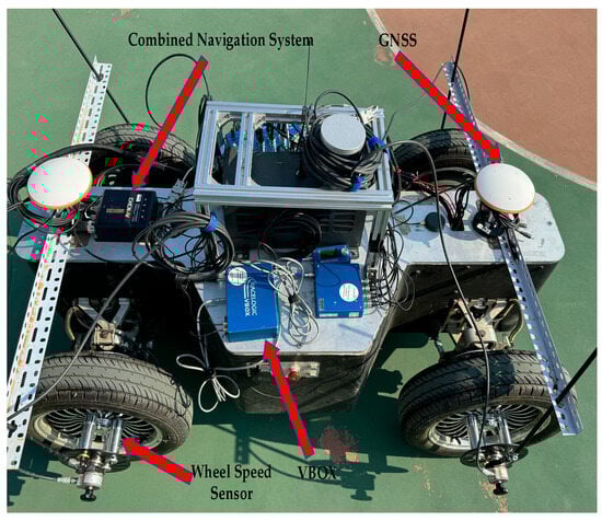
Figure 7.
Test vehicle and data acquisition equipment.
The school basketball court is selected as the test site to ensure that the test site is open and the antenna could receive a certain number of satellites. The test scenario is illustrated in Figure 8. The test vehicle conducted a 10-m slalom test with a data acquisition frequency of 100 Hz.
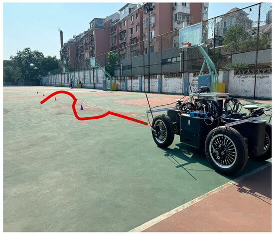
Figure 8.
Test scenario.
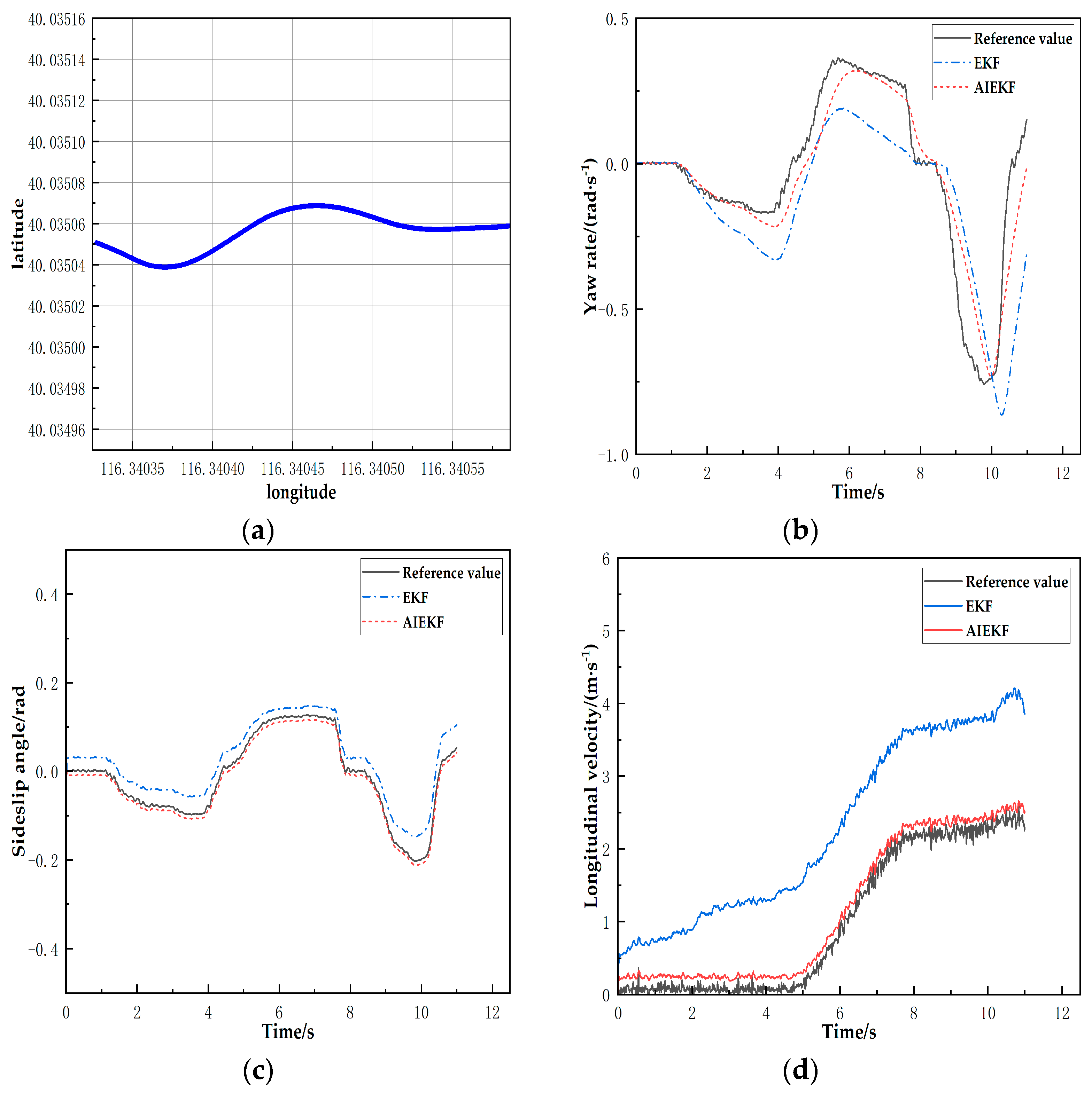
The experimental results show that the accuracy of the proposed AIEKF estimation algorithm is significantly higher than that of the EKF algorithm, especially in estimating the sideslip angle and the longitudinal velocity with less noise interference. As shown in Figure 9, during the initial slalom manoeuvre of the test vehicle, the rapid response of the steering wheel causes significant deviations in the yaw rate and sideslip angle estimated by the EKF algorithm. Additionally, the cumulative error increases with the duration of the steering, and the longitudinal velocity estimated by the EKF algorithm consistently shows an inevitable steady-state error throughout the test. In contrast, the AIEKF algorithm, due to its adaptive updating of the noise covariance matrix and ability to reduce stage errors, could quickly and accurately track the changing trends of state parameters during continuous steering of the test vehicle. Additionally, the estimation results have relatively small errors compared to the test data, with the maximum relative errors for the estimated sideslip angle and longitudinal speed being 23.02% and 17.43%, respectively. The results indicate that the AIEKF estimation algorithm has good accuracy and stability under the test condition and meets the requirements for control precision.
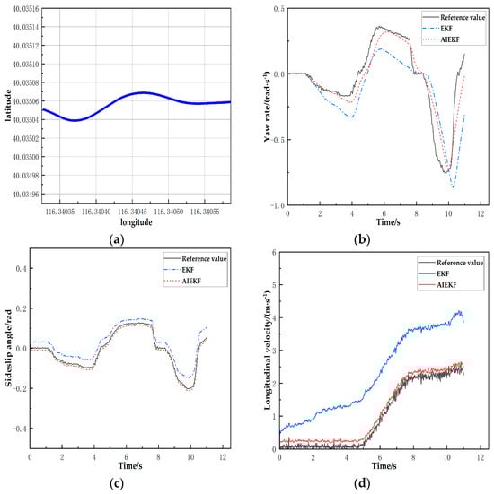
Figure 9.
Experimental results of vehicle state estimation: (a) latitude and longitude trajectory map of the test vehicle; (b) variation result of yaw rate; (c) variation result of sideslip angle; (d) variation result of longitudinal velocity.
To validate the accuracy of the proposed AIEKF algorithm in vehicle state estimation, the Mean Absolute Error (MAE) and Root Mean Square Error (RMSE) are applied as the metrics to test and quantify the accuracy of the estimation values. The expression is defined as follows
Meanwhile, to further validate the accuracy of the proposed AIEKF algorithm in estimating vehicle state parameters, a paired sample t-test will be conducted between the errors of AIEKF and the reference values, as well as the errors of EKF and the reference values, to compare whether there is a significant difference in the means of the two data sets. The test type is a two-tailed test, with a significance level set at α = 0.05. The formula for calculating the t-value is as follows.
where is the sample mean of the differences, is the sample standard deviation of the differences, and is the number of paired samples.
According to the results in Table 2 and Table 3, the estimation accuracy of the vehicle state parameters using the AIEKF algorithm is significantly higher than that of the EKF algorithm. In terms of assessing indicators, there is a significant decrease in the MAE and RMSE. In simulations and tests, the AIEKF algorithm improved the estimation accuracy of the yaw rate by 78.37% and 58.17%, respectively, compared to the EKF algorithm. Additionally, the estimation accuracy of the sideslip angle has been improved by 57.2% and 70.79%, and the estimation accuracy of the longitudinal speed has been improved by 76.47% and 87.11%. According to the results in Table 4, the t-values obtained from each data set are compared with the corresponding critical values in the t-distribution table to draw conclusions. There is a significant difference between the deviations of AIEKF and EKF. Therefore, it indicates that the AIEKF algorithm significantly improves the accuracy of vehicle state estimation compared to the EKF algorithm.
Table 2.
MAE indicators with different algorithms.
Table 3.
RMSE indicators with different algorithms.
Table 4.
The t-values with different data sets.
5. Discussion
As we all know, conventional research methods are based on accurate tire cornering stiffness and noise covariance matrices. However, parameter changes could degrade accuracy or even diverge the filter. To improve the estimation accuracy, our study first uses the recursive least squares method with variable forgetting factor (VFFRLS) to identify the tire cornering stiffness, and the iterative extended Kalman filter (IEKF) is used as the basic algorithm for vehicle state estimation. At the same time, we employ an innovative algorithm to optimise the uncertain noise covariance of the process. The algorithm compensates for the lack of consideration of the tire cornering stiffness and EKF estimation bias in the existing relevant literature.
The accuracy of the proposed algorithm is verified by simulation and experiment. From the results with MAE, RMSE indicators, and t-test, it is obvious that the estimation accuracy of the proposed AIEKF algorithm is significantly higher than that of the EKF algorithm. The reason is that the AIEKF algorithm considers the variation in the vehicle’s tire cornering stiffness, as well as the effect of the EKF-generated stage error and the adaptive adjustment of the observation noise. From the results, it can be seen that the deviation of the experiment is higher than the deviation of the simulation. The reason is that the simulation uses a high-precision vehicle model based on CarSim2019, which is a high-degrees-of-freedom vehicle model, but also makes some simplifying assumptions relative to the actual vehicle and has modelling errors. In the experiment, the estimation accuracy is reduced compared to the simulation because the vehicle is affected by several noises, such as environmental changes. However, the maximum relative error still meets the requirement of control accuracy.
The application of the AIEKF algorithm provides an idea for reducing the use of high-precision sensors and the cost of the whole vehicle. At the same time, it gives more reliable state information for studying vehicle handling stability and decision-making control in autonomous driving vehicles. However, the simulation and experimental results show that the AIEKF algorithm still has some deviations, which may have originated from the modelling error of the vehicle and tire models. Future research could be devoted to constructing more accurate vehicle and tire models and consider the influence of environmental factors, such as road slope and surface adhesion coefficient, to reduce the uncertainty error and further validate the algorithm’s accuracy through a real vehicle test in complex working conditions.
6. Conclusions
A fixed tire cornering stiffness setting affects the estimation accuracy in the vehicle state estimation process. Uncertainty noise could lead to the degradation of accuracy or even dispersion of the recognition results. To solve the problem, this study proposes the state estimation algorithm that combines the recursive least squares method with a variable forgetting factor and adaptive iterative extended Kalman filter. The process takes the identification results of cornering stiffness as the algorithm’s input and optimises the extended Kalman filter, which effectively reduces the impact of noise by updating the observation noise covariance matrix with online adjustments.
The proposed AIEKF algorithm is validated by co-simulation and experiment. The premise parameters are utilised to effectively estimate the yaw rate, the sideslip angle, and the longitudinal velocity of the vehicle under typical driving conditions. The simulation results show that the proposed AIEKF algorithm improves the estimation accuracy by 78.37%, 57.2%, and 76.47%, respectively, compared with the EKF algorithm. The experimental results show that the proposed AIEKF algorithm improves the estimation accuracy by 58.17%, 70.79%, and 87.11%, respectively, compared to the EKF algorithm. The new algorithm significantly enhances the ability to suppress observation noise and demonstrates robust stability.
Author Contributions
Conceptualisation, Y.C. and Y.H.; data curation, Y.H.; formal analysis, Y.H.; methodology, Y.C. and Y.H.; project administration, Y.C.; software, Y.H.; validation, Y.C. and Y.H.; visualization, Y.H.; writing—original draft, Y.H.; writing—review and editing, Y.C. and Z.S. All authors have read and agreed to the published version of the manuscript.
Funding
This research was funded by Project for capacity construction of science and technology innovation service, Beijing laboratory construction, Beijing Laboratory for New Energy Vehicles (PXM2021_014224_000065).
Data Availability Statement
The original contributions presented in the study are included in the article, further inquiries can be directed to the corresponding author.
Conflicts of Interest
The authors declare no conflicts of interest.
References
- Phadke, S.B.; Shendge, P.D.; Wanaskar, S.V. Control of antilock braking systems using disturbance observer with a novel nonlinear sliding surface. IEEE Trans. Ind. Electron. 2020, 67, 6815–6823. [Google Scholar] [CrossRef]
- Mousavinejad, E.; Han, Q.L.; Yang, F.; Zhu, Y.; Vlacic, L. Integrated control of ground vehicles dynamics via advanced terminal sliding mode control. Veh. Syst. Dyn. 2017, 55, 268–294. [Google Scholar] [CrossRef]
- Jin, X.; Yin, G.; Chen, N. Advanced estimation techniques for vehicle system dynamic state: A survey. Sensors 2019, 19, 4289. [Google Scholar] [CrossRef] [PubMed]
- Cheli, F.; Sabbioni, E.; Pesce, M.; Melzi, S. A methodology for vehicle sideslip angle identification: Comparison with experimental data. Veh. Syst. Dyn. 2007, 45, 549–563. [Google Scholar] [CrossRef]
- Selmanaj, D.; Corno, M.; Panzani, G.; Savaresi, S.M. Vehicle sideslip estimation: A kinematic based approach. Control Eng. Pract. 2017, 67, 1–12. [Google Scholar] [CrossRef]
- Grigorescu, S.; Trasnea, B.; Cocias, T.; Macesanu, G. A survey of deep learning techniques for autonomous driving. J. Field Robot. 2020, 37, 362–386. [Google Scholar] [CrossRef]
- Srinivasan, S.; Sa, I.; Zyner, A.; Reijgwart, V.; Valls, M.I.; Siegwart, R. End-to-end velocity estimation for autonomous racing. IEEE Robot. Autom. Lett. 2020, 5, 6869–6875. [Google Scholar] [CrossRef]
- Napolitano Dell’Annunziata, G.; Ruffini, M.; Stefanelli, R.; Adiletta, G.; Fichera, G.; Timpone, F. Four-Wheeled Vehicle Sideslip Angle Estimation: A Machine Learning-Based Technique for Real-Time Virtual Sensor Development. Appl. Sci. 2024, 14, 1036. [Google Scholar] [CrossRef]
- Guo, H.; Cao, D.; Chen, H.; Lv, C.; Wang, H.; Yang, S. Vehicle dynamic state estimation: State of the art schemes and perspectives. IEEE/CAA J. Autom. Sin. 2018, 5, 418–431. [Google Scholar] [CrossRef]
- Liu, Y.H.; Li, T.; Yang, Y.Y.; Ji, X.W.; Wu, J. Estimation of tire-road friction coefficient based on combined APF-IEKF and iteration algorithm. Mech. Syst. Signal Process. 2017, 88, 25–35. [Google Scholar] [CrossRef]
- Chen, Z.; Sun, H.; Dong, G.; Wei, J.; Wu, J.I. Particle filter-based state-of-charge estimation and remaining-dischargeable-time prediction method for lithium-ion batteries. J. Power Sources 2019, 414, 158–166. [Google Scholar] [CrossRef]
- Chu, W.; Luo, Y.; Dai, Y.; Li, K. In–wheel motor electric vehicle state estimation by using unscented particle filter. Int. J. Veh. Des. 2015, 67, 115–136. [Google Scholar] [CrossRef]
- Zhu, J.; Wang, Z.; Zhang, L.; Zhang, W. State and parameter estimation based on a modified particle filter for an in-wheel-motor-drive electric vehicle. Mech. Mach. Theory 2019, 133, 606–624. [Google Scholar] [CrossRef]
- Zhang, Y.; Ma, J.; Zhao, X.; Liu, X.; Zhang, K. A modified unscented Kalman filter combined with ant lion optimization for vehicle state estimation. Math. Probl. Eng. 2021, 2021, 8847075. [Google Scholar] [CrossRef]
- Gang, L.I.; Deyang, Z.; Ruichun, X.I.E. Vehicle state estimation based on improved Sage-Husa adaptive extended Kalman filter. Automot. Eng. 2017, 37, 1146–1432. [Google Scholar]
- Wang, Y.; Xu, L.; Zhang, F.; Dong, H.; Liu, Y.; Yin, G. An adaptive fault-tolerant EKF for vehicle state estimation with partial missing measurements. IEEE/ASME Trans. Mechatron. 2021, 26, 1318–1327. [Google Scholar] [CrossRef]
- Li, L.; Jia, G.; Ran, X.; Song, J.; Wu, K. A variable structure extended Kalman filter for vehicle sideslip angle estimation on a low friction road. Veh. Syst. Dyn. 2014, 52, 280–308. [Google Scholar] [CrossRef]
- Liu, Y.; Chen, H.; Wu, S.; Gao, J.; Li, Y.; An, Z.; Mao, B.; Tu, R.; Li, T. Impact of vehicle type, tyre feature and driving behaviour on tyre wear under real-world driving conditions. Sci. Total Environ. 2022, 842, 156950. [Google Scholar] [CrossRef]
- Pacejka, H. Tire and Vehicle Dynamics; Elsevier: Amsterdam, The Netherlands, 2005. [Google Scholar]
- Zheng, X.; Gao, X.; Zhao, Z. Simulation analysis of tire dynamic based on “Magic Formula”. Mach. Electron. 2012, 9, 16–20. [Google Scholar]
- Yuan, H.; Han, Y.; Zhou, Y.; Chen, Z.; Du, J.; Pei, H. State of charge dual estimation of a Li-ion battery based on variable forgetting factor recursive least square and multi-innovation unscented kalman filter algorithm. Energies 2022, 15, 1529. [Google Scholar] [CrossRef]
- Mao, Y.; Bao, J.; Zhang, Y.; Yang, Y. An Ultrafast Variable Forgetting Factor Recursive Least Square Method for Determining the State-of-Health of Li-ion Batteries. IEEE Access 2023, 11, 141152–141161. [Google Scholar] [CrossRef]
- Zerdali, E. A comparative study on adaptive EKF observers for state and parameter estimation of induction motor. IEEE Trans. Energy Convers. 2020, 35, 1443–1452. [Google Scholar] [CrossRef]
- Li, W.; Yang, Y.; Wang, D.; Yin, S. The multi-innovation extended Kalman filter algorithm for battery SOC estimation. Ionics 2020, 26, 6145–6156. [Google Scholar] [CrossRef]
- Chen, Y.; Yan, H.; Li, Y. Vehicle State Estimation Based on Sage–Husa Adaptive Unscented Kalman Filtering. World Electr. Veh. J. 2023, 14, 167. [Google Scholar] [CrossRef]
- Tang, Y.; Jiang, J.; Liu, J.; Yan, P.; Tao, Y.; Liu, J. A GRU and AKF-based hybrid algorithm for improving INS/GNSS navigation accuracy during GNSS outage. Remote Sens. 2022, 14, 752. [Google Scholar] [CrossRef]

Disclaimer/Publisher’s Note: The statements, opinions and data contained in all publications are solely those of the individual author(s) and contributor(s) and not of MDPI and/or the editor(s). MDPI and/or the editor(s) disclaim responsibility for any injury to people or property resulting from any ideas, methods, instructions or products referred to in the content. |
© 2024 by the authors. Published by MDPI on behalf of the World Electric Vehicle Association. Licensee MDPI, Basel, Switzerland. This article is an open access article distributed under the terms and conditions of the Creative Commons Attribution (CC BY) license (https://creativecommons.org/licenses/by/4.0/).