Abstract
In response to the problem of low optimization efficiency and low tracking accuracy in vehicle path tracking, a comprehensive optimization method is established based on the 3-DOF vehicle motion model. The outer layer adopts the adaptive particle swarm optimization (APSO) method for parameter optimization, and improves the adaptive inertia weight and adaptive particle exploration rate to improve the convergence efficiency and global search ability of the population. The inner layer adopts the segmented Gaussian pseudospectral method (GPM) to optimize the vehicle motion trajectory, and sets continuity constraints to ensure the continuity of the state and control variables at the segmentation points. The inner optimization results are fed back to the outer layer as a reference for the population updating fitness, achieving double-layer iterative optimization. The simulation results show that the proposed APSO-GPM optimization method can effectively solve the vehicle path tracking problem, with a high solving efficiency and stronger global optimization ability.
1. Introduction
With the increasing demand for safe, comfortable, energy-saving, and time-saving transportation services, many domestic and foreign automobile companies have invested a lot of manpower and material resources in the research of intelligent driving vehicles. Intelligent vehicles combine the characteristics and advantages of intelligent manufacturing technology and wire-controlled electric vehicle technology, which can not only reduce the pressure faced by drivers in complex driving environments, but also significantly improve the safety and comfort of vehicle driving. The horizontal and vertical control of intelligent vehicles are among the core technologies of intelligent driving, which can be used to process planned trajectories and vehicle position information, and output corresponding control commands to ensure that the vehicle travels along the predetermined trajectory. However, how to ensure that vehicles travel accurately along the planned trajectory and achieve the expected tracking accuracy is a major challenge in the field of intelligent vehicles. The continuous development of vehicle intelligence and electronic technology has greatly promoted the vigorous development of the automotive industry. How to improve the trajectory tracking, driving safety, and stability of intelligent vehicles has become a focus of research for many automotive companies. Accurately tracking complex paths is one of the necessary conditions for achieving stable vehicle operation. The goal of path tracking control is to make the vehicle travel according to a predetermined reference trajectory, that is, to control the vehicle to travel along the reference trajectory as much as possible through certain control methods, ensuring the handling stability of the vehicle and the comfort of the driver and passengers during driving. Path tracking control is a core component of intelligent vehicle autonomous driving technology, but there are strong nonlinear and time-varying characteristics in the vehicle path tracking system, which require a high dynamic performance of the control algorithm. How to improve the tracking accuracy and robustness of the controller is an important problem that urgently needs to be solved. Driving stability is an important factor affecting safety and comfort. A series of path tracking control algorithms have been developed to address these coupled optimization objectives. The autonomous vehicle puts forward high requirements for the accuracy of path tracking control; that is, it cannot deviate from the target path under all working conditions. Even if the road conditions are wet or the road is winding, the controller must have the ability to accurately track the target path, also known as the accuracy of path tracking, which is one of the important evaluation indicators of the path tracking algorithm [1,2,3].
Chen et al. designed a linear quadratic regulator (LQR) control strategy to improve the tracking accuracy of vehicles [4]. Ren et al. adopted the minimum model error criterion to reduce the estimation error of the observer and designed an adaptive sliding mode controller based on the observer [5]. Liang et al. used radial basis function neural networks to compensate for prediction errors, improving the tracking accuracy of vehicles on complex curvature changing roads [6]. Zhang et al. designed an MPC based on the nonlinear functions of the tire sideslip angle and slip ratio, which improved the tracking accuracy on low adhesion road surfaces [7]. In summary, the biggest limitation of model predictive control algorithms is the large amount of online computation and sensitivity to model uncertainty [8,9]. Wu et al. considered the uncertainty of tire lateral stiffness in controller design and designed a trajectory tracking controller based on robust predictive control [10]. However, the controller did not consider the influence of longitudinal vehicle speed on control performance, and online optimization was time-consuming. Cheng et al. proposed an online optimization method and an offline calculation method for predicting controllers based on linear matrix inequality (LMI) models, but ignored the influence of external disturbances on tracking performance, and the offline calculation method required known system state variables, which carried a conservative risk [11]. Dong et al. designed a robust H ∞ tracking controller, but did not consider the nonlinear characteristics of tires in the controller design [12]. In order to improve the stability, maneuverability, and comfort of vehicles during path tracking, and ensured that the performance of AFS and DYC could be fully utilized throughout the entire control process, many research experts had studied the joint control of AFS and DYC using different control methods. Liu et al. proposed a lateral dynamic control system that coordinated AFS and DYC, reducing lateral offset and heading angle deviation, effectively mitigating the inherent chattering problem of traditional SMC control [13]. Sang Nan et al. designed an active disturbance rejection integrated controller and divided it into control regions for active front wheel steering and direct yaw moment control, ensuring the performance of the two controllers when acting alone and the smoothness of the vehicle when switching between cooperative working modes [14]. Yao et al. proposed a coordinated controller that utilized stability judgment by applying the SOFM neural network and K-means algorithm. By weighting the coordinated system based on vehicle stability level, they proposed a coordinated controller that could achieve both tracking accuracy and handling stability [15]. Zhang et al. studied a path tracking control method that adapted to multi-parameter changes, improving the real-time robustness of intelligent driving vehicle path tracking control [16]. Kong et al. designed a lateral preview driver model with sliding mode control as the control objective to improve lateral stability, which increased the path tracking stability of the vehicle under high-speed conditions [17]. Chen et al. proposed multiple trajectory prediction driver models based on autonomous driving, which improved the robustness of the controller [18]. The above scholars were all studying front wheel steering path tracking control. Single front wheel steering path tracking control had problems such as large tracking errors and low stability on high-speed and low-adhesion roads. Therefore, four-wheel steering has become a research hotspot for improving path tracking control. Chen et al. proposed an improved grey wolf optimization–double adaptive extended Kalman filter algorithm based on a temperature-dependent second-order RC-equivalent circuit model [19]. Ni et al. proposed a Q-learning-based multi-strategy integrated artificial bee colony algorithm to address the issue of the monotonous and one-dimensional search strategy [20]. Rocha et al. proposed a hybrid genetic search for the traveling salesman problem [21]. Akopov proposed real-coded genetic algorithms for the multi-objective optimization problem [22]. Akopov et al. proposed a parallel hybrid biobjective genetic algorithm for traffic improvement [23]. Chai et al. proposed a novel swarm-intelligence-based algorithm for the optimal overtaking trajectory problem of vehicles [24]. Recently, an MPC method was used for the vehicle path tracking problem [25,26,27,28]. Several approaches [29,30,31] had been introduced to implement optimize-based schemes in real time which could be used to address potential computational constraints. In Reference [29], Chachuata et al. surveyed different ways of using measurements to compensate for model uncertainty in the context of process optimization. In Reference [30], Hosseinzadeh et al. developed a robust to early termination optimization approach that can be used to effectively solve onboard optimization problems. In Reference [31], Adetola et al. proposed a controller design approach that integrated RTO and MPC for the control of constrained uncertain nonlinear systems.
In summary, although there have been many studies on the problem of vehicle path tracking, some of the methods provided in the literatures have a low solving accuracy, and some research methods have a low solving efficiency. This article proposes a dual-layer comprehensive optimization method for the problem of vehicle path tracking. The rest of the article is organized as follows: Section 2 presents the problem of vehicle path tracking, while Section 3 describes the comprehensive optimization method. Section 4 presents numerical simulations and experimental verification. Finally, Section 5 concludes the main work of the article.
2. Vehicle Path Tracking Problem
2.1. Mathematical Model of Vehicle Path Tracking Problem
A nonlinear 4-DOF vehicle model shown in Figure 1 is used to describe the vehicle path tracking problem.
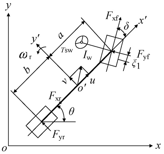
Figure 1.
4-DOF vehicle model.
In the state space form, the equation is as follows [1]:
The state variable is and the control variable is . Then, Equation (2) can be obtained by simplifying Equation (1).
2.2. Optimal Control Object of Path Tracking Problem
The minimum time required to complete the path tracking process is determined as the control object.
The cost function is as follows:
where is the initial time, and is the final time.
2.3. Tire Model
The lateral forces of the front and rear wheels can be expressed as follows [32]:
where and are the lateral stiffness values of the front and rear tires. and are the front and rear slip angles.
2.4. Constrains
The initial and terminal states are described as follows:
When the braking maneuver is applied to decelerate the vehicle, the constraints on , can be rewritten in the following manner:
Therefore, the optimal path tracking problem can be described as follows:
where expresses the inequality constraint.
3. Comprehensive Optimization Method
This article designs a double-layer iterative optimization algorithm to solve the comprehensive optimization problem. The outer layer uses APSO to search for static parameters as the overall parameter input for the inner layer trajectory optimization. The inner layer adopts the GPM and the SQP method to solve the trajectory optimization problem. And the optimization result is used as the fitness required for the updating of the outer particle swarm forming a double-layer iterative optimization algorithm. This can not only reduce the coupling between the parameter optimization problem and the trajectory optimization problem, but also achieve the satisfaction of process constraints and handover point equality constraints, thereby obtaining a convergent solution.
3.1. Adaptive Particle Swarm Optimization Algorithm
The particle swarm optimization (PSO) algorithm solves problems by simulating the mutual transmission and sharing of food location information among birds during their foraging process, thereby adjusting their own state towards the goal. It utilizes the mechanism of information sharing among biological populations to promote the development of the entire population. The PSO algorithm has excellent global optimization characteristics and does not require obvious gradient characteristics.
This article proposes an adaptive inertia weight APSO algorithm, which endows each particle with an adaptive random exploration desire to enhance their exploration ability and overcome the disadvantages of a slow convergence speed and easy falling into local optimum, improving the optimization speed and accuracy.
In APSO, each particle is considered as an independent solution in the solution space. And the dimension of the particle depends on the number of optimization variables. If the population size is set as M, the position of the ith () particle can be denoted as , with a velocity of . The position experienced by the particle with the highest fitness is denoted as the historical optimal position of the particle. And the position of the particle with the highest fitness in the entire population is denoted as the global optimal position. The position and velocity of any particle are updated according to Equation (10):
where is the inertia weight; and are the learning factors which are usually taken as fixed normal numbers; and represents the random number generated on the interval of [0, 1]. In Equation (14), the first equation represents the three parts of the velocity update, which, respectively, represent the previous velocity of the particle and the cognition of the current position, as well as the particle search process. This reflects the characteristics of particle swarm optimization, including local search, global search, and information sharing.
On the basis of PSO, APSO designs the inertia weight as a dynamic function that continuously changes with fitness, improving the efficiency of solving. The objective function obtained from the inner layer optimization is set as the fitness, which is denoted as , representing the fitness obtained by the ith particle in the dth iteration. The expression of the inertia weight is as follows:
where and are the preset minimum and maximum inertia coefficients, respectively; is the average fitness of the population in the dth iteration; and is the maximum fitness of the population in the dth iteration.
This article defines the adaptive random exploration rate of particles as which is designed as a dynamic function that adapts with the number of iterations:
where and represent the maximum and minimum exploration rates, respectively; is the maximum number of iterations for random exploration, satisfying , where is the maximum number of the iterations.
The meaning of Equation (12) is to endow particles with a greater desire to explore in the early stage and achieve global search and avoid becoming stuck in local optimal solutions. As exploration progresses, the desire for particle exploration gradually decreases and the ability for local search improves. The updating formula for particle velocity with as exploratory ability is as follows:
where is the proportion coefficient of the random exploration speed of particles to the maximum search speed ; is the random number satisfying the standard normal distribution; and represents the random numbers on the interval .
Equation (13) indicates that particles with a desire to explore will randomly search in the direction with velocity .
3.2. Segmented Gaussian Pseudospectral Method
This article uses the segmented Gauss pseudospectral method to transform the trajectory optimization problem of a vehicle into a nonlinear programming problem, which is solved using the sequential quadratic programming method.
On interval , the discretization steps of the segmented Gaussian pseudospectral method are as follows:
- (1)
- Time-domain normalization
The Gauss pseudospectral method discretizes the state and control variables at the Legendre–Gauss (LG) point. Due to the LG point being located between (−1,1), Equation (14) needs to be used for time-domain conversion:
- (2)
- Approximation of global interpolation polynomial
K + 1 nodes are composed of K collocation points of the Gauss pseudospectral method (roots of K-order Legendre polynomials) and . The state variable is approximated by a Lagrange polynomial based on K + 1 nodes:
where is the actual state variable at time; is the approximate state variable at time; is the discrete state variable at time; and is the Lagrange interpolation basis function.
The approximate expression of the control variable is as follows:
where is the actual control variable at time; is the approximate control variable at time; is the discrete control variable at time; and is the Lagrange interpolation basis function.
- (3)
- Constraint transformation
Equation (18) can be obtained by taking the derivative of Equation (15) at the pth collocation point.
where ; is the differential difference matrix.
It is set that the derivative of Equation (18) is equal to the right-hand function of the state variable. And, then, the constraint of the differential equation is transformed into an algebraic constraint.
The terminal state needs to satisfy the dynamic constraints, which can be obtained by integrating the initial state with the dynamic equation. The integral part is approximated by Gauss integration:
where is the weight value at the p collocation point.
The boundary constraints and path constraints are discretized into the following form:
- (4)
- Performance index
Equation (23) can be obtained by approximating the integral term with the Gauss integral.
The overall performance indicator is as follows:
In order to ensure the continuity of the trajectory and control variables, the state variables, time nodes, and control variables should also satisfy the following relationships:
In summary, the optimization problem of the path tracking of a vehicle can be transformed into the optimal control problem of the segmented Gauss pseudospectral method for solving the objective function Equation (24), path constraint Equation (21), boundary constraint Equation (22), state equation constraint Equation (19), terminal state constraint Equation (20), and segmented connection point constraint Equation (25).
The scheme of the algorithm is shown in Figure 2.
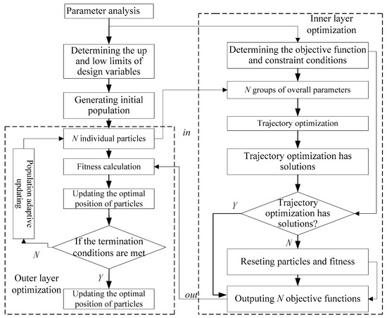
Figure 2.
Scheme of the algorithm.
4. Numerical Simulations and Experimental Verification
4.1. Numerical Simulations
A simulation is established under the double lane changing condition with different adhesion coefficients to verify the effectiveness of the algorithm.
4.1.1. Condition of
Figure 3 is the simulation result of the lateral distance and the yaw rate under the condition of . It can be seen from Figure 3a that there are small errors at the lateral distance of 60 m and 80 m, that is, at the turns of the double lane changing road. However, the vehicle can track the given path well, with the control of the proposed algorithm indicating a good control performance.
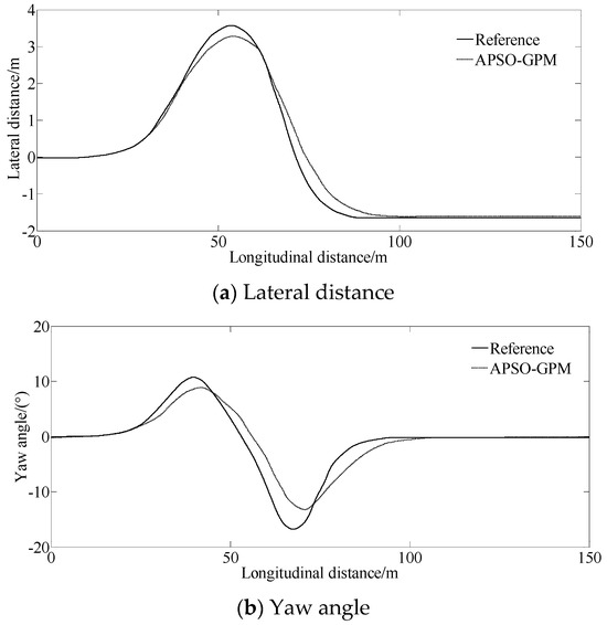
Figure 3.
Simulation result under condition of .
This is because the adaptive inertia weight and adaptive exploration rate of the proposed algorithm can improve the autonomy and exploration efficiency of particles and improve the convergence speed of the population, and also avoid local convergence. From Figure 3b, it can be seen that there are peak values at 40 m and 70 m of the lateral distance. This is because the vehicle needs a higher yaw angle to ensure the vehicle stability. However, the simulation curve maintains consistency with the reference, indicating the effectiveness of the proposed idea.
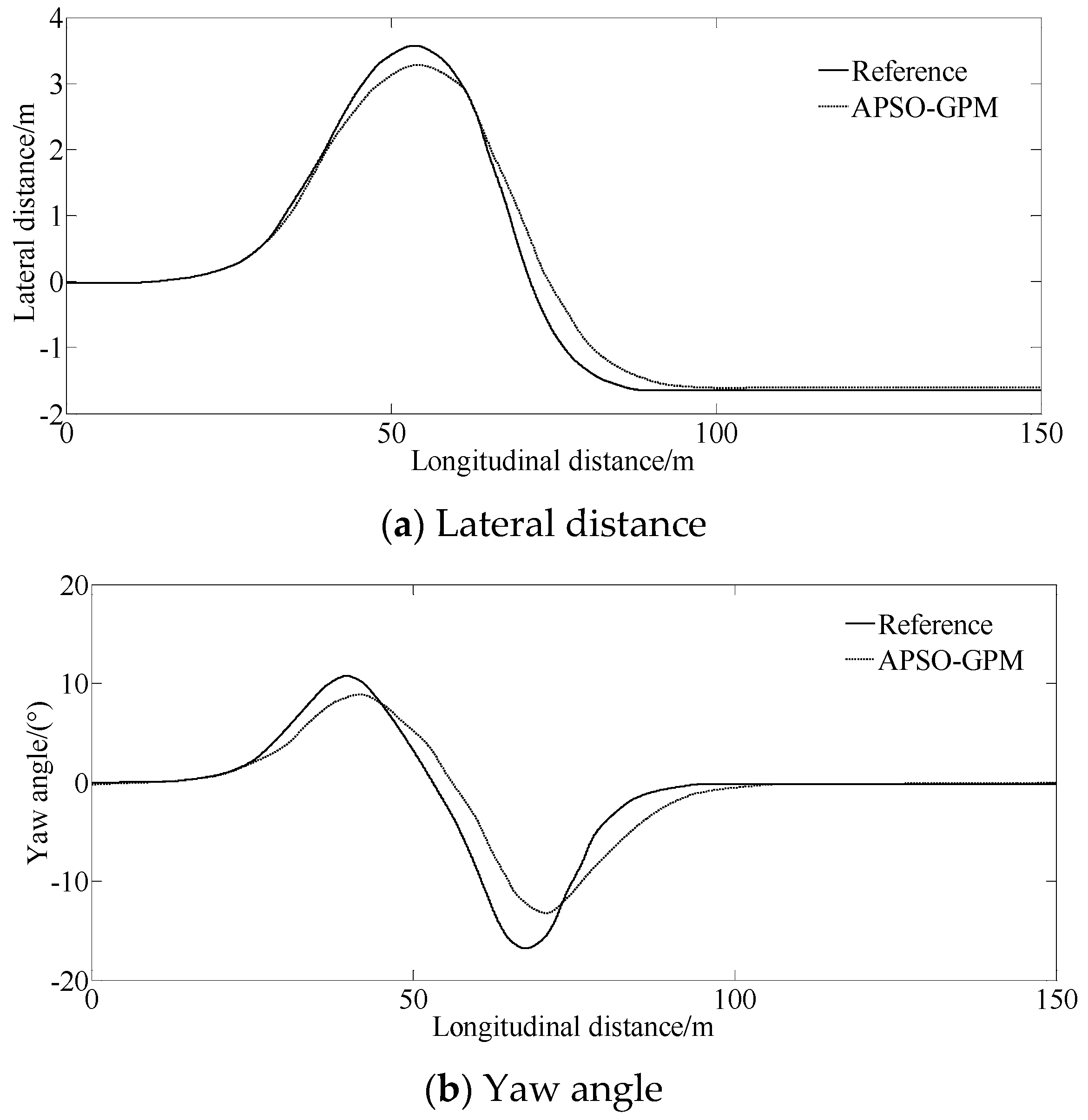
4.1.2. Condition of
Figure 4 is the simulation result of the lateral distance and the yaw rate under the condition of . It can be seen from Figure 4a that there are errors at the lateral distance of 60 m and 80 m. And, moreover, it can be seen that, when the adhesion coefficient becomes smaller, the error between the simulation result and the reference become larger. From Figure 4b, it can be seen that there are peak values at 40 m and 65 m of the lateral distance. And moreover, it can be seen that, when the adhesion coefficient becomes smaller, the error between the simulation result and the reference become larger.
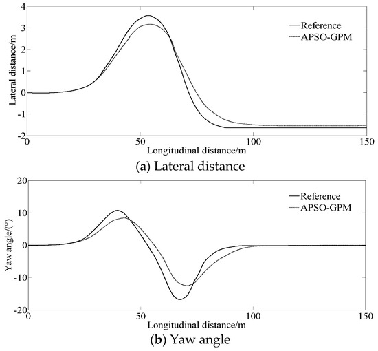
Figure 4.
Simulation result under condition of .
4.2. Accuracy Verification
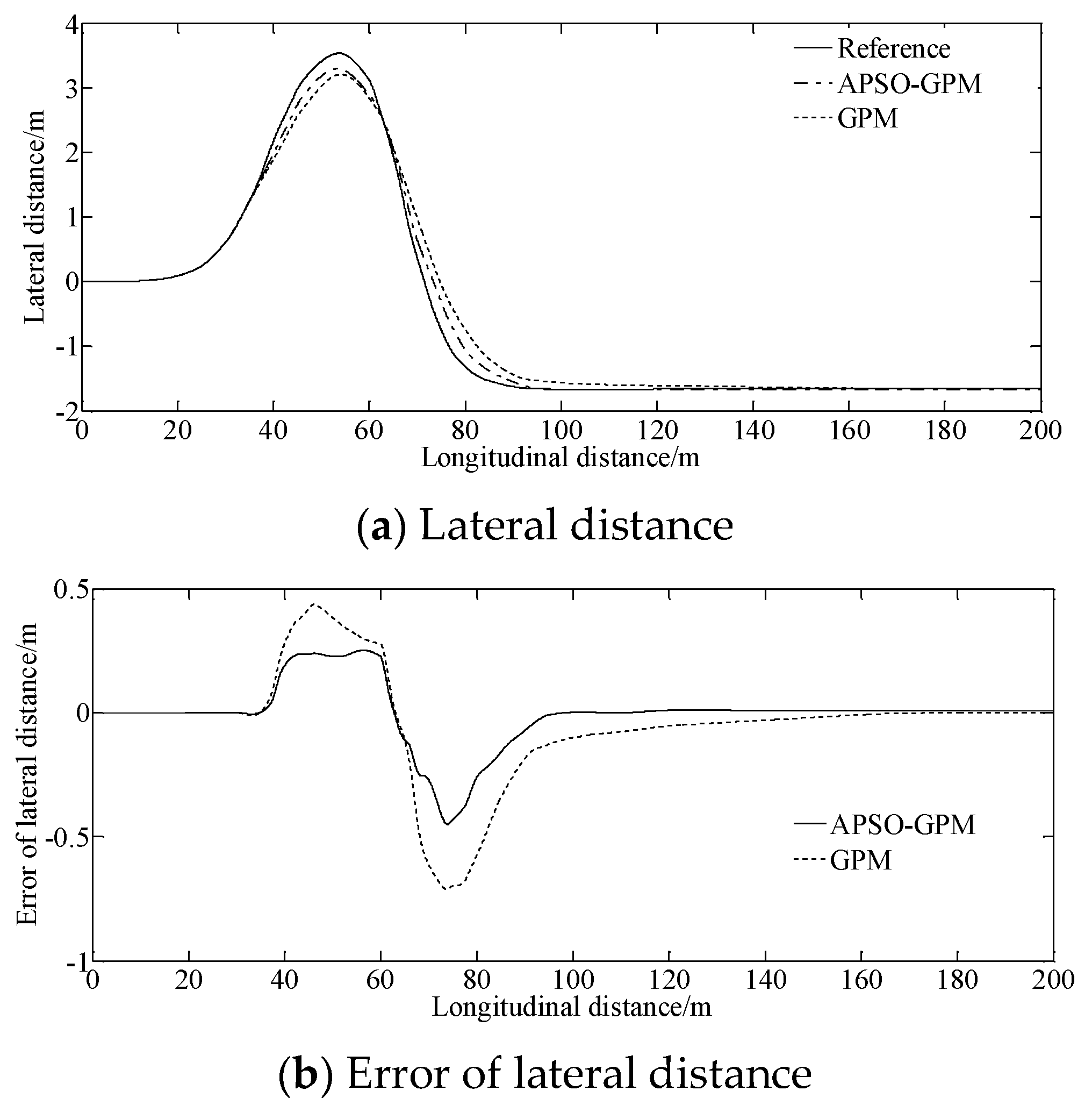
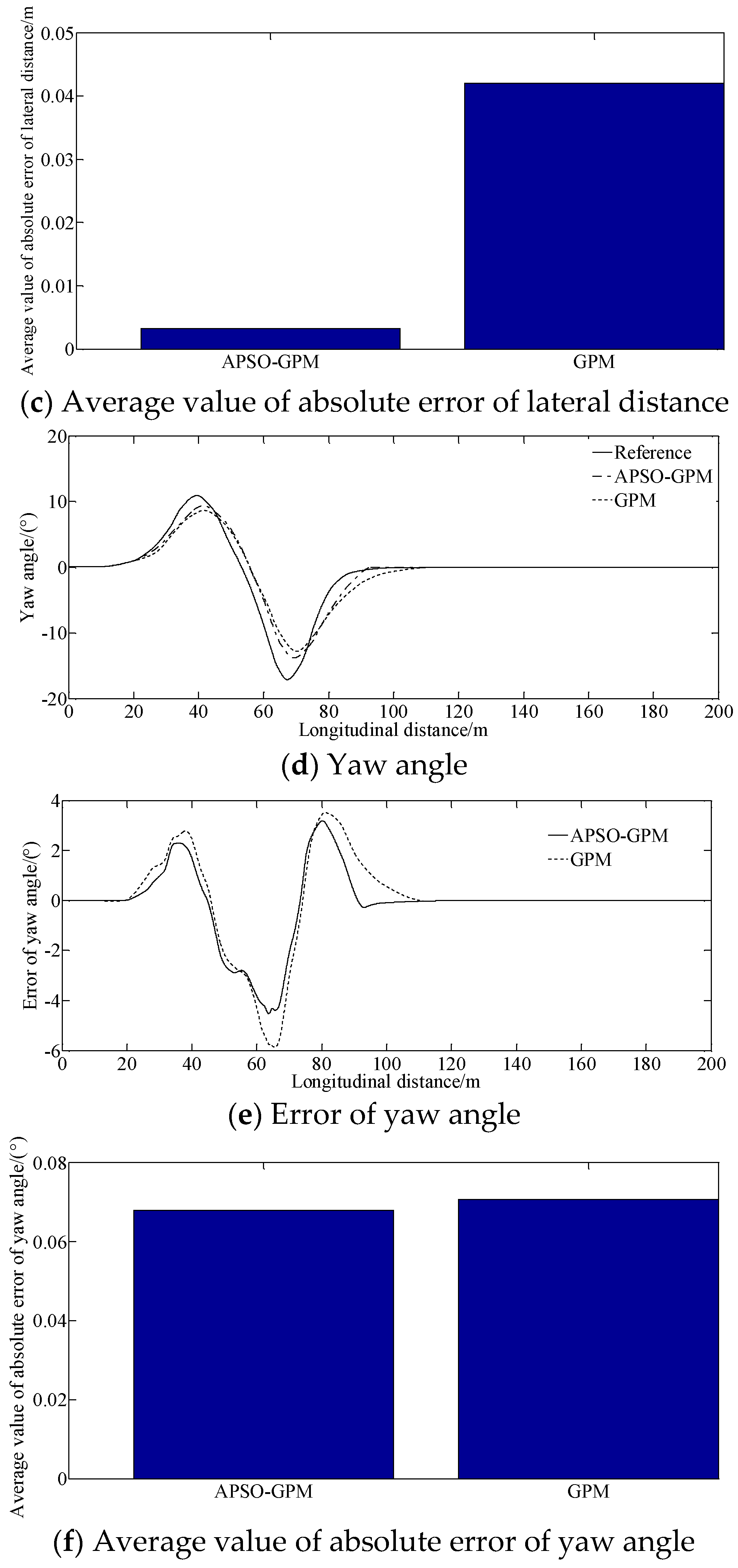
Figure 5 is the result of the lateral distance for accuracy verification. It can be seen that, when tracking the same given path under the same conditions, the error between the reference and the simulation value of the APSO-GPM algorithm is smaller than that of the MPC method, indicating a higher calculation accuracy. Table 1 is the comparison of the average value of the absolute error between the different methods. Table 2 is the number of iterations and CPU time of the two methods.

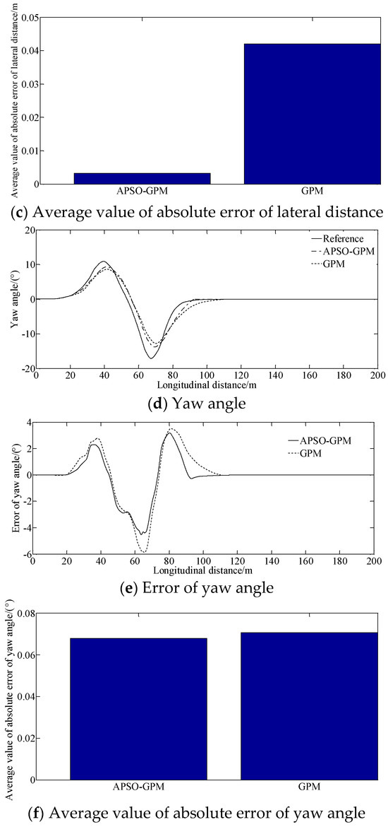
Figure 5.
Accuracy and efficiency verification.

Table 1.
Comparison of average value of absolute error between different methods.
Table 2.
Comparison of the number of iterations and CPU time of each method.
Figure 5c,f and Table 1 show that, compared with the traditional GPM method, the proposed algorithm can control the vehicle to track the given path well, maintaining a good tracking accuracy.
It can be seen from Table 2 that the number of iterations and the CPU time of the APSO-GPM are lower than that of the traditional GPM, indicating the better solving efficiency and higher convergence rate of the proposed method.
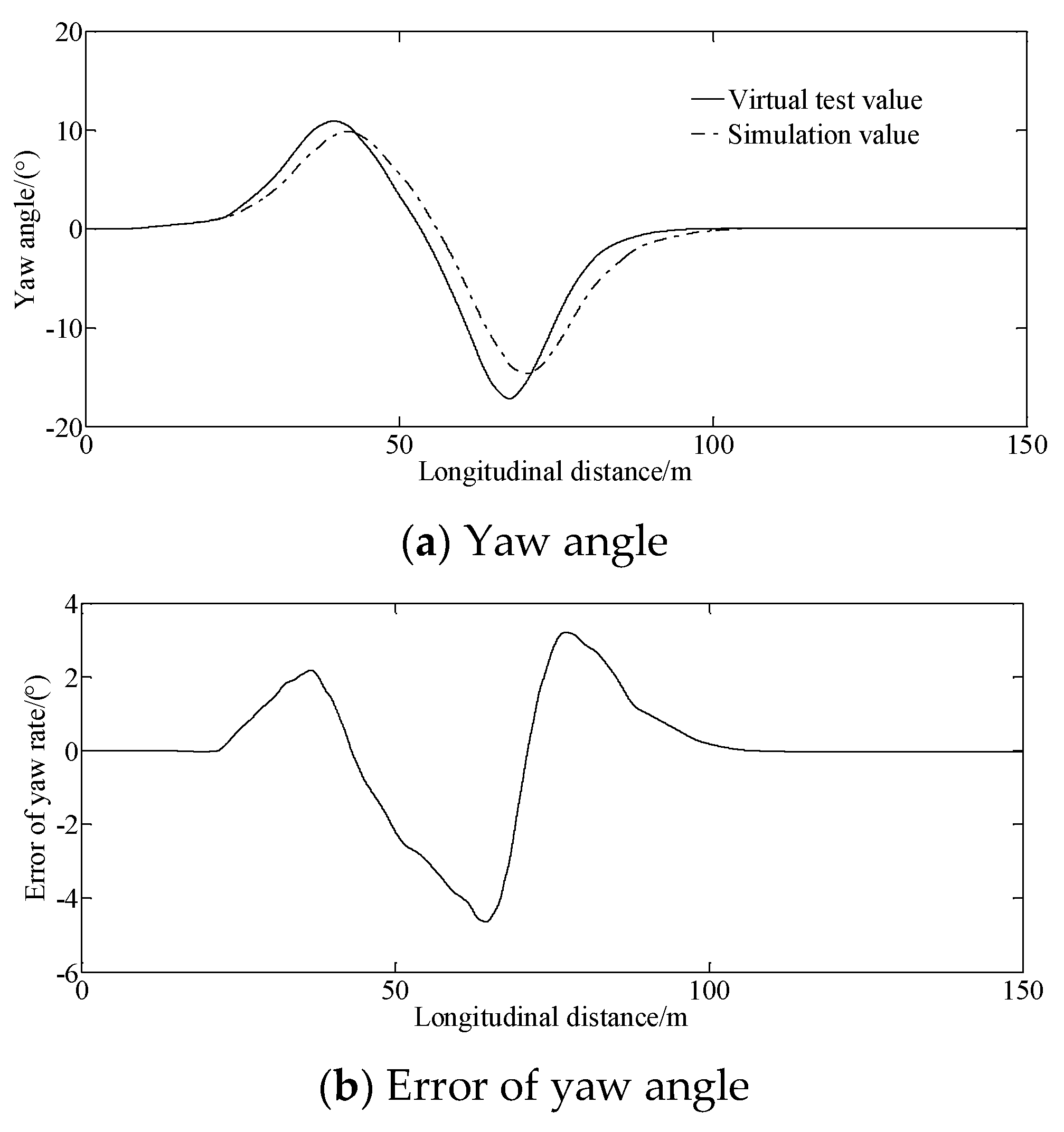
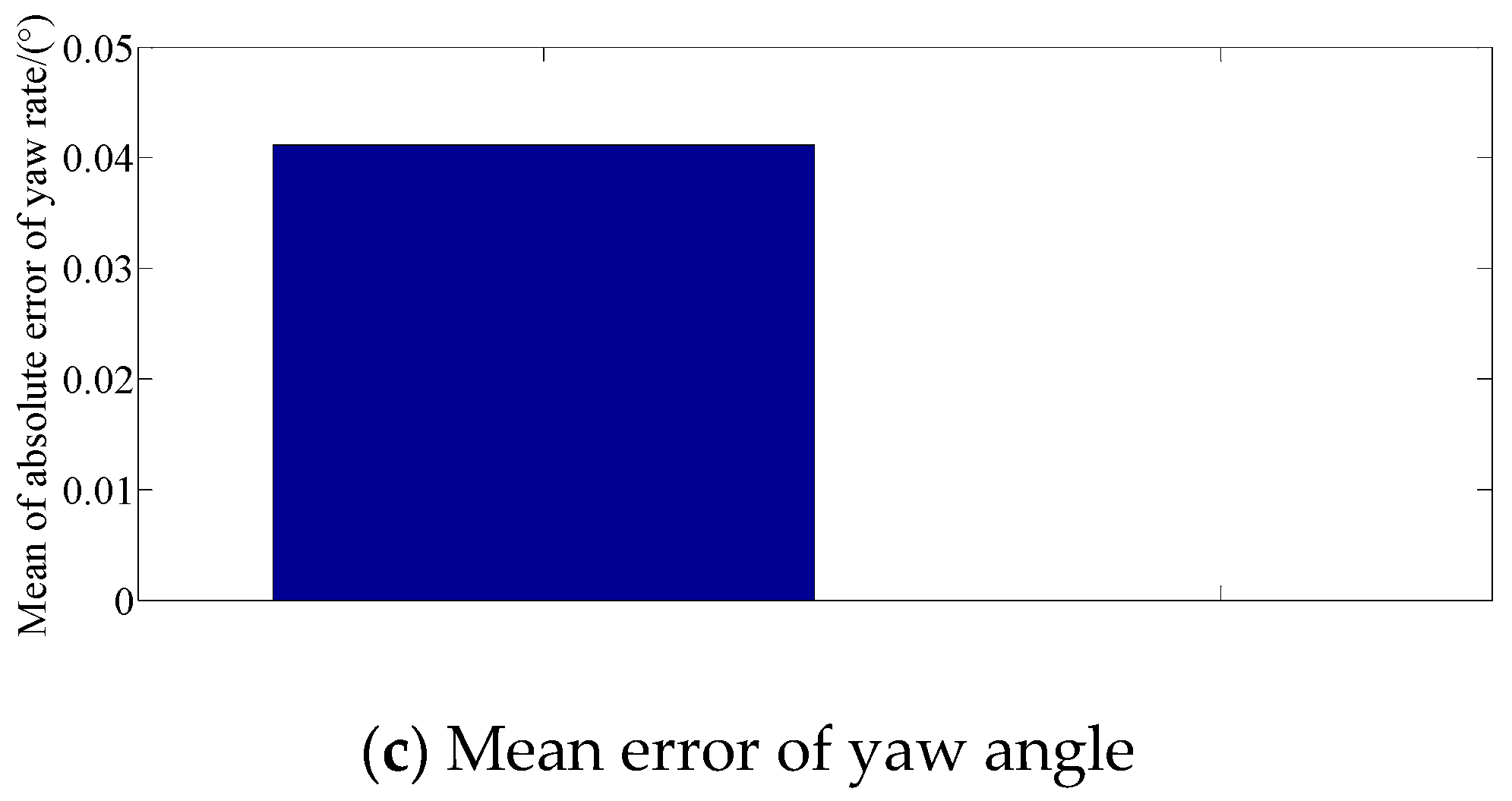
4.3. Experimental Verification
A virtual test adopting the CarSim R2019 software is conducted to verify the feasibility of the simulated results.
CarSimR2019 is a simulation software specifically designed for vehicle dynamics, which can respond to the driver, different road conditions, and aerodynamic inputs. It simulates the autonomous driving function by setting parameters for various systems of the vehicle and customizing algorithms. The simulation results are played through 3D animation, and data analysis graphics are generated to help users understand specific functions. Its powerful backend data, including vehicle models, operating conditions, and autonomous driving algorithms, allow users to complete a simulation exercise in a short period of time and observe data results in real time. CarSim R2019 can also be well-integrated with mathematical models, such as conducting joint simulations with MATLAB/Simulink to establish autonomous driving algorithm models and gain a deeper understanding of autonomous driving functions. CarSim R2019 software, as the mainstream software for automotive kinematic simulation, comes with various experimental models and has good scalability. It can be connected with external software such as Simulink to conduct relevant testing.
Figure 6 is the experimental result of the yaw angle. It is shown that there are errors between the simulation and the virtual test values. The reason is that the model in the virtual test ignores the nonlinearity of the steering system and suspension system. However, the mean of the absolute error of the yaw angle is 0.041 degrees. The trend of the curves and small error are enough to illustrate the correctness of the proposed method.
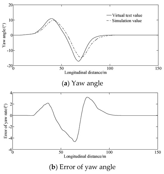
Figure 6.
Experimental results of yaw angle.
5. Conclusions
In order to solve the problem of vehicle path tracking, this article designs an APSO-GPM double-layer iterative optimization algorithm to solve the problem of vehicle trajectory tracking. The designed double-layer iterative framework enables the optimization algorithm to have a good convergence. The improved adaptive inertia weight and adaptive exploration rate APSO method further enhances the convergence speed and optimization ability of the optimization algorithm. The theoretical analysis and simulation results indicate that the double-layer iterative optimization method can effectively solve the optimization problem of vehicle trajectory tracking. And, moreover, the APSO has a stronger global search capability and higher search efficiency. The segmented GPM can effectively solve trajectory optimization problems that satisfy the process and terminal constraints, improving the solution efficiency.
The performance of the APSO algorithm deteriorates as the dimensionality of the problem to be solved increases. In the future, whether the algorithm allows the solving of this problem by distributing the processing among several processors of a computer system will be researched.
Author Contributions
Methodology, Y.L.; software, D.C. All authors have read and agreed to the published version of the manuscript.
Funding
This research was supported by the Open Research Program of Huzhou Key Laboratory of Urban Multidimensional Perception and Intelligent Computing under Grant No. UMPIC202404.
Data Availability Statement
The related data used to support the findings of this study are available from the corresponding author upon request.
Acknowledgments
This research was supported by the Open Research Program of Huzhou Key Laboratory of Urban Multidimensional Perception and Intelligent Computing under Grant No. UMPIC202404. The authors gratefully acknowledge the support agency.
Conflicts of Interest
The authors declare no conflicts of interest.
References
- Liu, Y.J.; Cui, D.W.; Peng, W. Optimum Control for Path Tracking Problem of Vehicle Handling Inverse Dynamics. Sensors 2023, 23, 6673. [Google Scholar] [CrossRef] [PubMed]
- Liu, Y.J.; Cui, D.W.; Peng, W. Optimal Lane Changing Problem of Vehicle Handling Inverse Dynamics Based on Mesh Refinement Method. IEEE Access 2023, 11, 115617–115626. [Google Scholar] [CrossRef]
- Liu, Y.J.; Cui, D.W. Vehicle dynamics prediction via adaptive robust unscented particle filter. Adv. Mech. Eng. 2023, 15, 16878132231170766. [Google Scholar] [CrossRef]
- Chen, L.; Qin, Z.B.; Kong, W.W.; Chen, X. Lateral control using LQR for intelligent vehicles based on optimal front tire lateral force. J. Tsinghua Univ. Sci. Technol. 2021, 61, 906–912. [Google Scholar]
- Ren, Y.; Ji, J.; Zhao, Y.; Lang, Y.X.; Zheng, L. Path tracking control of intelligent vehicle based on minimal model error estimation. Automot. Eng. 2021, 43, 580–587. [Google Scholar]
- Qie, T.Q.; Wang, W.D.; Yang, C.; Li, Y.; Liu, W.; Xiang, C. A path planning algorithm for autonomous flying vehicles in cross-country environments with a novel TF-RRT* method. Green Energy Intell. Transp. 2022, 1, 100026. [Google Scholar] [CrossRef]
- Zhang, W.G.; Zhang, P.; Wei, H.; Xiong, J.Z. An improved path tracking control algorithm for autonomous vehicle based on LTVMPC. J. Hunan Univ. Nat. Sci. 2021, 48, 67–73. [Google Scholar]
- Wang, B.; Zhang, Y.M.; Zhang, W. Integrated path planning and trajectory tracking control for quadrotor UAVs with obstacle avoidance in the presence of environmental and systematic uncertainties: Theory and experiment. Aerosp. Sci. Technol. 2022, 120, 107277–107294. [Google Scholar] [CrossRef]
- Xie, L.T.; Xie, L.; Su, H.Y. Comparison of robust and stochastic model predictive control algorithms for uncertain systems. J. Autom. 2017, 43, 969–982. [Google Scholar]
- Wu, H.D.; Si, Z.L. Intelligent vehicle trajectory tracking control based on linear matrix inequality. J. Zhejiang Univ. Eng. Sci. 2020, 54, 110–117. [Google Scholar]
- Cheng, S.; Li, L.; Chen, X.; Wu, J. Model-predictive-control-based path tracking controller of autonomous vehicle considering parametric uncertainties and velocity-varying. IEEE Trans. Ind. Electron. 2020, 68, 8698–8707. [Google Scholar] [CrossRef]
- Dong, Q.; Ji, X.W.; Liu, Y.L.; Tao, S.; Liu, Y. Robust LPV/H∞ control for automatic path tracking of heavy commercial vehicles. J. Tsinghua Univ. Sci. Technol. 2022, 62, 438–446. [Google Scholar]
- Liu, J.; Gao, L.; Zhang, J.J.; Yang, F. Super-twisting algorithm second-order sliding mode control for collision avoidance system based on active front steering and direct yaw moment control. Proc. Inst. Mech. Eng. 2021, 235, 43–54. [Google Scholar] [CrossRef]
- Sang, N.; Liu, R.Q.; Zhao, W.Z. Coordinated control of active front steering and direct yaw moment for vehicles. J. Nanjing Univ. Sci. Technol. 2018, 42, 655–661. [Google Scholar]
- Yao, X.X.; Gu, X.G.; Jiang, P. Coordination control of active front steering and direct yaw moment control based on stability judgment for AVs stability enhancement. Proc. Inst. Mech. Eng. Part D J. Automob. Eng. 2022, 236, 59–74. [Google Scholar] [CrossRef]
- Zhang, L.X.; Wu, G.Q.; Guo, X.X. Path Tracking Using Linear Time-varying Model Predictive Control for Autonomous Vehicle. J. Tongji Univ. 2016, 44, 1595–1603. [Google Scholar]
- Kong, X.X.; Deng, S.W.; Yu, S.J.; Yi, Q.; Jin, Y.H. Driver Model of Vehicle Lateral Preview Based on Sliding Mode Control. J. Hubei Univ. Automot. Technol. 2020, 34, 25–28. [Google Scholar]
- Chen, W.W.; Tan, D.K.; Wang, H.B.; Wang, J.; Xia, G. A Class of Driver Directional Control Model Based on Trajectory Prediction. J. Mech. Eng. 2016, 52, 106–115. [Google Scholar] [CrossRef]
- Chen, L.; Wang, S.L.; Chen, L.; Gao, H.; Fernandez, C. An improved grey wolf optimization-double adaptive extended Kalman filtering algorithm for co-estimation of state of charge and state of health for lithium-ion batteries based on temperature-dependent second-order. RC Model. Ion. 2024, 30, 4631–4646. [Google Scholar] [CrossRef]
- Ni, X.R.; Hu, W.; Fan, Q.C.; Cui, Y.; Qi, C. A Q-learning based multi-strategy integrated artificial bee colony algorithm with application in unmanned vehicle path planning. Expert Syst. Appl. 2024, 236, 121303. [Google Scholar] [CrossRef]
- Rocha, Y.; Subramanian, A. Hybrid genetic search for the traveling salesman problem with hybrid electric vehicle and time windows. Comput. Oper. Res. 2023, 155, 106223. [Google Scholar] [CrossRef]
- Akopov, A.S. An Improved Parallel Biobjective Hybrid Real-Coded Genetic Algorithm with Clustering-Based Selection. Cybern. Inf. Technol. 2024, 24, 32–49. [Google Scholar] [CrossRef]
- Akopov, A.S.; Beklaryan, L.A. Traffic Improvement in Manhattan Road Networks with the Use of Parallel Hybrid Biobjective Genetic Algorithm. IEEE Access 2024, 12, 19532–19552. [Google Scholar] [CrossRef]
- Chai, R.; Tsourdos, A.; Savvaris, A.; Chai, S.; Xia, Y.; Chen, C.P. Multiobjective Overtaking Maneuver Planning for Autonomous Ground Vehicles. IEEE Trans. Cybern. 2021, 51, 4035–4049. [Google Scholar] [CrossRef]
- Bejarano, G.; Manzano, J.M.; Salvador, J.R.; Limon, D. Nonlinear model predictive control-based guidance law for path following of unmanned surface vehicles. Ocean. Eng. 2022, 258, 111764–111777. [Google Scholar] [CrossRef]
- Alejandro, G.G.; Ivana, C.G.; Rodolfo, C.U.; Sotelo, C.; Sotelo, D.; Castañeda, H. Path-following and LiDAR-based obstacle avoidance via NMPC for an autonomous surface vehicle. Ocean. Eng. 2022, 266, 112900–112907. [Google Scholar]
- Rokonuzzaman, M.; Mohajer, N.; Nahavandi, S. Effective adoption of vehicle models for autonomous vehicle path tracking: A switched MPC approach. Veh. Syst. Dyn. 2022, 61, 1236–1259. [Google Scholar] [CrossRef]
- Wang, M.; Chen, J.X.; Yang, H.W.; Wu, X.; Ye, L. Path Tracking Method Based on Model Predictive Control and Genetic Algorithm for Autonomous Vehicle. Math. Probl. Eng. 2022, 2022, 4661401. [Google Scholar] [CrossRef]
- Chachuata, B.; Srinivasanb, B.; Bonvinc, D. Adaptation strategies for real-time optimization. Comput. Chem. Eng. 2009, 33, 1557–1567. [Google Scholar] [CrossRef]
- Hosseinzadeh, M.; Sinopoli, B.; Kolmanovsky, I.; Baruah, S. Implementing Optimization-Based Control Tasks in Cyber-Physical Systems with Limited Computing Capacity. In Proceedings of the 2022 2nd International Workshop on Computation-Aware Algorithmic Design for Cyber-Physical Systems (CAADCPS), Milan, Italy, 3–6 May 2022; pp. 15–16. [Google Scholar]
- Adetola, V.; Guay, M. Integration of real-time optimization and model predictive control. J. Process Control 2010, 20, 125–133. [Google Scholar] [CrossRef]
- Liu, Y.J.; Cui, D.W.; Peng, W. Vehicle state and parameter estimation based on improved extend Kalman filter. J. Meas. Eng. 2023, 11, 496–508. [Google Scholar] [CrossRef]


Disclaimer/Publisher’s Note: The statements, opinions and data contained in all publications are solely those of the individual author(s) and contributor(s) and not of MDPI and/or the editor(s). MDPI and/or the editor(s) disclaim responsibility for any injury to people or property resulting from any ideas, methods, instructions or products referred to in the content. |
© 2024 by the authors. Published by MDPI on behalf of the World Electric Vehicle Association. Licensee MDPI, Basel, Switzerland. This article is an open access article distributed under the terms and conditions of the Creative Commons Attribution (CC BY) license (https://creativecommons.org/licenses/by/4.0/).