Abstract
A trajectory planning method is proposed to address the lane-changing problem in intelligent vehicles. The method is based on quintic polynomial improvement. The transit position is determined according to the position and state of motion of the vehicle and the obstacle vehicle; the lane-changing process is divided into two segments. The quintic polynomials are commonly applied in trajectory planning, respectively, in the two segments. According to the different characteristics of the lane-changing paths in the front and rear segments, a multi-objective optimization function with different weight coefficients is established. A safe and comfortable lane-changing trajectory is achieved through the improved particle swarm optimization algorithm. Real-time simulation tests of lane-changing method are conducted on the hardware-in-the-loop platform. The method can be used in different scenarios to plan safe and comfortable trajectories.
1. Introduction
Self-driving vehicles can fulfill most of the operations of human drivers and reduce traffic accidents caused by improper operation of human drivers [1]. According to relevant studies, it is predicted that the popularization of self-driving technology can reduce the rate of automobile accidents by more than 90% and significantly improve road traffic safety [2,3]. As a prevalent driving action when intelligent vehicles drive automatically, lane-changing behavior that is safe, fast and smooth can improve the efficiency of passage and reduce the incidence of traffic accidents [4].
Reasonable lane-changing trajectory is a prerequisite for intelligent vehicles to accomplish the lane-changing task safely [5]. Trajectory planning for self-driving vehicles is the core technology to ensure safe and efficient driving, and with the increase in complexity and dynamics of the traffic environment, trajectory planning algorithms need to be efficient, robust and adaptive [6]. The current mainstream methods are systematically categorized into five groups: graph search methods search for optimal paths by constructing environment maps (e.g., raster maps) and search algorithms (e.g., A* algorithms), which are suitable for static environments but have high computational complexity [7]; sampling methods (e.g., RRT, PRM) generate paths by random sampling, which are suitable for high-dimensional spaces and dynamic environments, but the paths may not be smooth enough [8]; geometric methods use geometric curves (e.g., polynomial curves) to generate smooth trajectories that satisfy dynamical constraints [9]; optimal control-based methods generate high-quality trajectories by solving optimization problems, but are computationally burdensome [10]; and learning-based methods use machine learning (e.g., reinforcement learning) to learn planning strategies from data, which is adaptive, but data acquisition and model generalization capabilities are still challenges [11,12]. The performance comparison of different planning algorithms is summarized in Table 1.

Table 1.
Comparison of planning algorithms.
Out of the techniques previously described, the geometric method has the easiest computational process compared to the other methods, which can generate smooth trajectories that satisfy the kinematic constraints through simple computations, and thus polynomial curves are a popular choice for trajectory planning. Low-order polynomials (e.g., cubic polynomials) can satisfy the continuity of position and velocity and are often used in simple trajectory planning problems. The literature [13] proposes a trajectory planning method via discrete cubic polynomial curves to identify the optimal path by adjusting the vehicle’s location in a defined area. Higher order polynomials (e.g., sixth or higher order) can satisfy higher order dynamics constraints and are suitable for high-speed motion or scenarios that require very high trajectory smoothness, but the computation becomes complicated as the order increases. The literature [14] proposes a trajectory planning algorithm using a sixth-order polynomial for obstacle avoidance based on vehicle kinematics equations. However, this algorithm suffers from high computational complexity and slow convergence due to higher order and more coefficients to be determined. The lane-changing trajectory planned using quintic polynomials can effectively balance the smoothness of the trajectory and computational efficiency. Compared with the low-order polynomials, quintic polynomials can satisfy the continuity requirements of position, velocity and acceleration, and generate smoother trajectories. Meanwhile, a quintic polynomial has lower computational complexity compared with higher-order polynomials, which can quickly generate trajectories in scenes with high real-time requirements. The literature [15] proposes a path planning algorithm via polynomial functions, which sets the acceleration constraints and establishes a polynomial parameterized simulation model with velocity boundaries and path time optimization, which provides a reference for the subsequent research on dynamics models. The literature [16] proposes a real-time path planning method via quintic polynomial optimization, which generates smooth and dynamically constrained trajectories by quintic polynomials and combines the optimization algorithm to achieve real-time and safety, applied to the trajectory generation of self-driving vehicles in complex traffic environments.
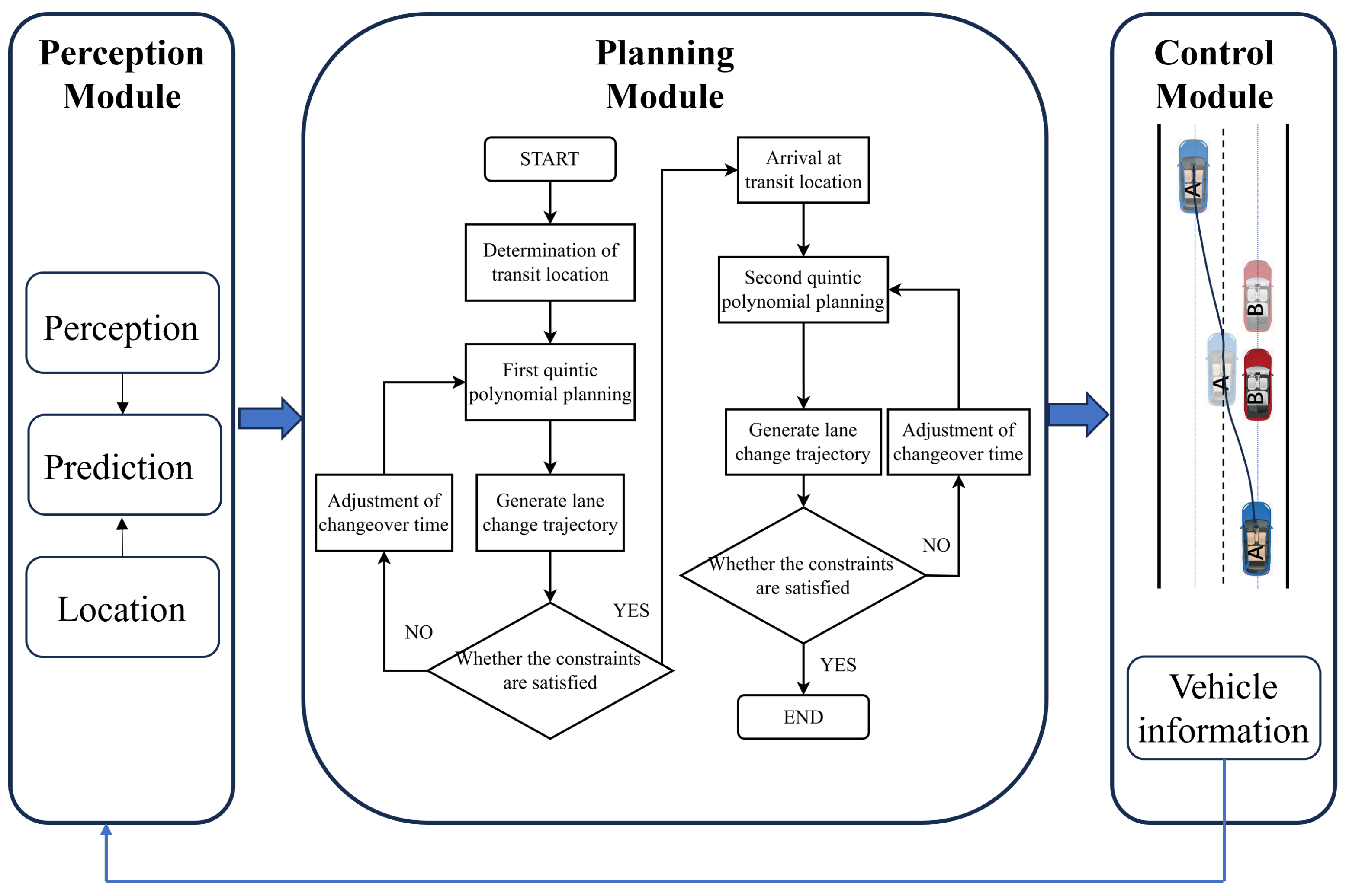
Quintic polynomials are commonly applied in lane-changing path planning due to unique advantages; however, the traditional quintic polynomial model is commonly used to increase the order of the constraint equations in obstacle avoidance and lane changing to satisfy the demands of vehicle dynamics limitations and driving performance. The method is computationally cumbersome, which can lead to an increase in planning time and a decrease in safety [17]. To solve the above problems, an intelligent vehicle lane-changing path planning method via improved quintic polynomial is proposed. The process of lane-changing is segmented into two parts before and after by setting a suitable transit position. Then, according to the different characteristics of the two paths, a multi-objective optimization objective function with different weight coefficients is established, and a secure and comfortable lane-changing trajectory is obtained through optimization algorithm. The proposed framework for lane-changing path planning in self-driving cars is graphically represented in Figure 1.
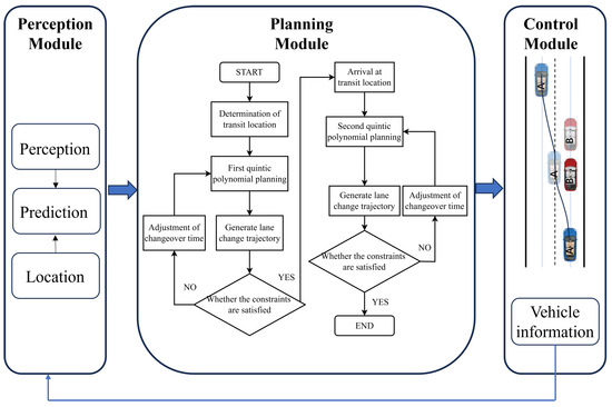
Figure 1.
The framework diagram of the strategy.
Contributions of this article:
(1) Via the traditional quintic polynomial planning for lane-changing trajectory planning, it is proposed to increase the staging position and change it into segmented planning for lane-change trajectory. By analyzing the critical collision state of the intelligent car and the obstacle car in front, and at the same time considering the state of the two cars to determine the transit position, it is ensured that there is no collision risk between the intelligent car and the obstacle car when changing lanes.
(2) Establish multi-objective optimization functions with different weighting coefficients according to the different characteristics of the paths at the front and rear ends, which are used to adjust the lane-changing time. Improve the optimization algorithm by integrating genetic algorithm in particle swarm algorithm to accelerate the convergence process, and enhance the diversity of solutions and global search ability, so that the optimization algorithm has stronger adaptability and robustness.
(3) In addition to static and dynamic obstacle vehicle scenarios, the validation algorithm adds the validation in low adhesion coefficient roadway scenarios, which ensures that the lane-changing model has wide applicability.
2. Problem and Scenario Descriptions
This paper mainly centers on the lane-changing and obstacle-avoiding behavior of self-driving vehicles. When the self-driving vehicle cruises at a certain speed in the lane, when there is an obstacle vehicle in front of the lane that affects the normal passage of the vehicle, the self-driving vehicle takes the initiative to change lanes according to a safe and comfortable lane-changing trajectory that is planned so as to avoid the obstacle vehicle in front of it and continue to drive normally.
A typical scenario of a self-driving vehicle changing lanes to avoid obstacles is shown in Figure 2:

Figure 2.
Typical scenario of lane-changing obstacle avoidance.
Figure 2 shows a typical unidirectional two-lane highway lane-changing scenario; two same direction lanes are a super lane (fast lane) and an ordinary lane, both lane widths are 3.75 m. Intelligent vehicle A, the front obstacle vehicle B and the rear vehicle C are all driving in the right ordinary lane, and the left front vehicle D and the left rear vehicle E are all driving in the left lane. According to traffic rules as well as actual driving habits, vehicle lane-changing to avoid obstacles generally chooses to change lanes from the current lane to the neighboring lane on the left side, so the left overtaking lane is the target lane for the self-driving vehicle A. As the relative longitudinal distance between intelligent vehicle A and vehicle B decreases, intelligent vehicle A has to perform the lane-changing operation to avoid the potential collision danger with the vehicle in front of it, B.
The focus of this paper is to study the lane-changing trajectory planning for self-driving vehicles to avoid the obstacle vehicles in front of them, so it is assumed that the lane-changing vehicles are only affected by the obstacle vehicles in front of them, except that they are not affected by other vehicles in the surrounding area, and the scenarios are simplified as follows.
(1) Vehicle A has sufficient space to change lane to the target lane (vehicle D and vehicle E will not affect vehicle A’s lane change).
(2) Rear vehicle C has also been travelling at a safe distance from vehicle A and will not affect vehicle A’s lane-changing operation.
(3) Vehicle A is travelling at a safe distance from vehicle B in front of it before changing lanes, and the effect of longitudinal speed on transverse speed is ignored during the lane change.
Eventually, the simplified lane-changing collision avoidance scenario is shown in Figure 3.

Figure 3.
Simplified scenario.
Via the simplified scenario, we plan lane-changing trajectories of smart car A that encounters obstacle car B in front of it.
3. Modeling of Lane-Change Trajectory Planning
3.1. Conventional Quintic Polynomial Lane-Change Model
After the above simplification of scenario, when the intelligent vehicle A needs to change lanes to avoid the obstacle vehicle B in order to continue normal driving, the lane-changing path planning mainly considers the vehicle A to avoid collision with the obstacle vehicle B during the lane-changing process. The intelligent vehicle A can choose a quintic polynomial curve based on time as a parameter of the lane-changing trajectory when it executes instruction to change lane.
In Figure 3, vehicle A is about to perform the lane-changing operation. Vehicle A drives from the centerline position of the lane it is in to the target position on the centerline of the adjacent target lane. When using the quintic polynomial curve as the planning trajectory curve of the vehicle lane change, we only need to know the start state and the end state of the intelligent vehicle A. After calculation, we can get a smooth quintic polynomial curve as the obstacle avoidance trajectory of the intelligent vehicle.
The start state and the goal state of smart vehicle A are
where x, , , y, and are the displacement, speed and acceleration of vehicle A in longitudinal as well as transversal direction, respectively.
The commutative trajectory functions in the x- and y-directions are computed as follows:
where and are the coefficients to be determined for the trajectory function in the x and y directions, respectively; t is time; means longitudinal state function; is transverse state function.
Combining Equations (1) and (2), the quintic polynomial commutative channel model can be expressed as
where T is the time parameter matrix and and are the longitudinal and transverse state vectors, respectively.
Define the time parameter matrix T as follows:
where is the initial moment of channel change; is the moment of channel change completion.
Define the coefficient matrices of the longitudinal and transverse state functions A and B, respectively, as follows:
At the starting moment of lane-changing, the displacement, speed and acceleration of vehicle A in the transverse direction are zero. After the longitudinal distance L, vehicle A completes the lane change, and its target state has a displacement of W in the transverse direction and zero velocity and acceleration in the transverse direction. The trajectory function should satisfy the following boundary conditions:
where for the starting moment; for the ending moment; , for the beginning and end of vehicle A speed, respectively; W is usually taken as the standard high-speed lane width of 3.75 m; L for the longitudinal displacement; assuming that the longitudinal speed of vehicle A is unchanged when changing lanes, then .
By setting the boundary conditions, it can be ensured that not only the speed is continuous without sudden change between the starting and ending positions of the planning path, but also the acceleration is continuous without sudden change, which improves the smoothness of traveling when vehicle A is changing lanes, and enhances passenger comfort.
Combining the boundary conditions and other constraints of Equation (6), and then combining Equations (3)–(5), the coefficient matrices A and B in Equation (5) can be found:
After obtaining the coefficient matrices A and B, the final lane-changing trajectory function is achieved through combining Equations (2) and (3).
In traditional quintic polynomial planning, if the initial speed and the final speed of the lane-changing vehicle are determined, the lane-changing time T is the only remaining variable to be considered, and the final lane-changing trajectory function can be obtained via the boundary conditions and constraints [18].
3.2. Improved Quintic Polynomial Lane-Change Model
Traditional lane-change trajectory planning using quintic polynomial curves not only requires a large safety distance, but also takes a long time to change lanes. In order to solve the defects of using a single quintuple polynomial, we propose a double-quintic polynomial lane-changing trajectory planning algorithm via the quintic polynomial. By adding a transitional state in the lane-changing process, the original lane-changing process is segmented into two parts. The transit position not only acts as the end point of the first planning, but also the starting point of the second planning, thus obtaining the lane-changing trajectory composed of two quintuple polynomial curves. The lane-changing process is shown in Figure 4, where vehicle A is the intelligent vehicle that needs to perform lane-changing, and vehicle B is the obstacle vehicle in front of the original lane.

Figure 4.
Improved channelization process.
Vehicle A arrives at the expected staging position at the end of the first planning, at which time vehicle A maintains a safe distance from the right front obstacle vehicle B in the transverse direction. Thereafter, when the lane-changing vehicle A performs the second planning, not only is it no longer intersecting with the obstacle vehicle B in the longitudinal direction, but also the distance in the transverse direction is increasing, and there is no risk of collision with the obstacle vehicle B in the transverse and longitudinal directions.
After smart vehicle A reaches the transit location of the transition, it performs five times polynomial path planning again via the transit state and the final goal condition at this time, as shown in Figure 5:

Figure 5.
Diagram of the second lane change.
Adding a suitable transition staging location to divide the lane-changing process into two phases significantly improves the safety of intelligent vehicles during the lane-changing phase.
3.2.1. Solving for Transit Position
Selecting the appropriate transition staging location is the difficulty. The selection of the transit position needs to consider the speeds of the lane-changing vehicle A and the obstacle vehicle B ahead, the distance between the two vehicles, the displacement of the lane-changing vehicle A, and the width of the obstacle vehicle B ahead, in conjunction with lane-change safety distance modeling.
It is assumed that during the local planning cycle of lane-changing path planning, the intelligent vehicle A is cruising normally at a certain speed. The perception system module of the intelligent vehicle obtains the motion status information of the obstacle vehicle B ahead, as well as the position state information through the sensors. A right-angle coordinate system is constituted with the center of mass of the vehicle in the initial state of lane-changing of the intelligent vehicle as the coordinate origin and the centerline of the initial lane as the X-axis, from which the state of the obstacle vehicle B ahead in the following period of time can be determined.
Taking the transit position as the demarcation point, the lane-changing process of the intelligent vehicle is segmented into two successive stages. In the first stage, the intelligent vehicle travels from the initial position of lane-changing to the mid-turn position, and only needs to move the appropriate lateral displacement to complete the obstacle avoidance task for the obstacle vehicle in front; in the second stage, the intelligent vehicle travels from the mid-turn position to the target position, and since there is no risk of collision between the lane-changing vehicle and the obstacle vehicle in this stage, the second lane-changing path planning can be regarded as the lane-changing path planning under the barrier-free situation.
At time , at this time the lane-changing vehicle A has just completed the first stage of lane-changing planning and arrived at the transit position. At this time, vehicle A and the obstacle vehicle B are in the critical collision state, as shown in Figure 6a. In order to make the two vehicles have no risk of collision, the following needs to be satisfied:
where , are the horizontal coordinates of the center of mass of the obstacle vehicle B and the intelligent vehicle A at , respectively; is the distance from the center of mass of the intelligent vehicle A to the front of the vehicle; is the distance from the center of mass of the obstacle vehicle B to the rear of the vehicle; is the width of the vehicle A; and is the angle between the axis of the body of the intelligent vehicle A and the direction of the road at the end of the first planning.
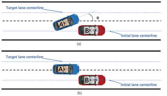
Figure 6.
Comparison of transit positions: (a) Theoretical transit point. (b) Transit point after ignoring heading angle.
In the actual process, the intelligent vehicle at the end of the first lane change has a very small angle between its body axis and the road, and its body is nearly parallel to the road. Therefore, the heading angle of vehicle A at the end of the first stage of planning can be ignored, assuming that the position of vehicle A at this time is at the transit position shown in Figure 6b.
That is, Equation (8) becomes the following:
Therefore, the state of smart vehicle A vehicle in the transit position is
where , , and are the transverse displacement, longitudinal displacement, and longitudinal velocity, respectively, of intelligent vehicle A when it is located in the transit position at the moment .
The is marginally broader than the width of the obstacle vehicle B ahead. According to the actual width of the obstacle vehicle B, adjustments are made, and the value is generally between 1.8 m and 2 m to ensure that the cars have a certain safety distance in the lateral direction. From this, we can get :
where is a constant between 1.1 and 1.2, the value is related to the condition of the two vehicles; is the width of the vehicle B.
The longitudinal displacement is determined via the lane-changing time in the first stage and the starting speed of vehicle A. The vehicle’s speed is hypothesized to remain constant while a short period of time is planned for. From this, is obtained:
The speed in the transition position is usually slightly greater than . In order to complete the lane change expeditiously, the vehicle making the lane change generally adopts the strategy to accelerate to make the lane change. There is a special situation, that is, if the front obstacle vehicle is in the stationary state, the lane change vehicle may be required to decelerate appropriately to make the longitudinal lane change; at this time, the transit speed needs to be slightly less than . From this, we can get :
where and denote the longitudinal velocity of car A at the transit moment and the initial moment, respectively, is a constant taking values between 0.8 and 1.4.
3.2.2. Modeling of Double-Quintic Polynomial Lane Change
After determining the appropriate transition staging position state function, and then combining the initial and goal states described in the previous section, the double quintuple polynomial path planning state can be obtained, as shown in Equation (13):
where , , are the initial state, the transitional transit state, and the final target state of the lane change, respectively; is the speed of vehicle A in the initial state of the lane change; , , , and , , are the longitudinal displacement, longitudinal velocity, and transverse displacement in the transit state and the final target state of the lane change.
The first phase of the lane change involves smart vehicle A traveling to the mid-turn position to avoid the obstacle vehicle in front of it, and the second phase involves smart vehicle A traveling from the mid-turn position to the final target position.
To acquire the coefficient matrices A and B in Equation (3), the longitudinal speed at the staging position and the lane-changing time at the first stage can be used as the optimization variables. and can be taken in a range of values according to the condition of the two vehicles.
The starting condition of the front obstacle vehicle B vehicle is shown in Equation (15):
where is the speed of the vehicle B ( is less than ); is the distance between the two vehicles; is the acceleration of the vehicle B ().
Assuming that the center of mass of the two vehicles moves to the same position in the longitudinal direction after t time and the intelligent vehicle A maintains a constant speed within the shorter planning cycle, Equations (16) and (17) can be obtained:
where is the vehicle speed of the obstacle vehicle B after time t.
In real driving situations, the speed of the smart vehicle A usual varies, so solving Equation (16) yields the maximum lane-change time :
where p is the speed difference between the two vehicles; q is the distance of the two vehicles B ().
When the front obstacle vehicle B is not stationary and has a certain speed to travel, the first quintic polynomial lane-changing process is able to be subdivided into two phases. The first phase is the intelligent vehicle A traveling to the starting location of the obstacle vehicle B. In the second phase, the vehicle A travels to the end of the first quintic polynomial planning (i.e., the transition mid-range position).
Two times and are calculated based on the states of the lane-changing vehicle A and the obstacle vehicle B ahead:
Then, the total time for the first stage of lane-changing is
Determine the optimal range of values for depending on whether the front vehicle is stationary or in motion, respectively:
where, , are real numbers less than 1. When the obstacle vehicle in front is stationary, the lane-changing time must have a certain safety margin, which should be less than the theoretical maximum lane-changing time. In addition, to ensure safety, should also satisfy
When the front obstacle vehicle is stationary (i.e., both and are 0), at this time, the front obstacle vehicle stays where it is and does not continue to move forward. If the intelligent vehicle wants to avoid collision with it, it needs to satisfy Equation (9): .
In the second segment of the quintic polynomial trajectory planning, both the initial state and the final goal state are determined. Similar to traditional quintic polynomial programming, only the lane-changing time and longitudinal displacement need to be solved by the optimization algorithm.
4. Trajectory Optimization Based on GA-PSO Hybrid Algorithm
4.1. GA-PSO Hybrid Algorithm
Particle Swarm Optimization (PSO) is an optimization algorithm via group intelligence, which explores the optimal solution by simulating a group of “particles” interacting and collaborating in a search space [19]. The main advantage of PSO is its fast convergence speed and simple and easy-to-implement update mechanism. However, when the solution space is multi-peaked or of high complexity, the local search ability of PSO is weak.
The Genetic Algorithm (GA) is an optimization method based on heuristic principles, drawing inspiration from natural selection and biological evolution. It functions by emulating evolutionary mechanisms, wherein a group of potential solutions undergoes iterative refinement across multiple generations to identify optimal or near-optimal outcomes for complex problems. The process starts with an initial set of randomly generated individuals, each encoded as a chromosome representing a possible solution. Through repeated cycles of selection, crossover, and mutation, the population gradually evolves, enhancing fitness as measured by an objective function. A notable strength of GA lies in its capability to address non-linear, multi-modal, and high-dimensional optimization challenges, particularly in scenarios where traditional gradient-based techniques may struggle. Unlike deterministic methods, GA maintains a diverse population, enabling broader exploration of the search space and reducing the likelihood of getting trapped in local optima.
Compared with PSO, genetic algorithm GA performs more outstandingly in global search and can effectively avoid the search from falling into local optimum. Therefore, the genetic algorithm is embedded within the particle swarm optimization framework to enhance its capabilities:
(1) Selection operation: use roulette selection to retain particles with higher adaptation and eliminate particles with lower adaptation.
(2) Crossover operation: use arithmetic crossover to perform crossover operation on the selected particles to generate new particles:
where is a random number and and are selected particles.
(3) Mutation operation: using Gaussian variation, particles are randomly mutated to increase the diversity of the population.
(4) Retention of elite particles: in each iteration, the best-adapted particles are retained to avoid losing the optimal solution.
(5) Stagnation detection: if the global optimal solution does not change in multiple iterations, reset to avoid the algorithm from falling into local optimality.
In the proposed GA-PSO hybrid algorithm (Algorithm 1), the Gaussian variation probability is set to 0.1 (). This means that each selected particle has a 10% chance to undergo Gaussian mutation during each generation. The Gaussian perturbation is defined as follows:
where is the Gaussian standard deviation set to 5% of the search space length. The convergence of the GA-PSO algorithm is determined based on two conditions: (1) The algorithm terminates if the iteration number reaches a predefined maximum, . (2) Early termination when the global optimal solution does not improve significantly (i.e., ) within 20 consecutive generations.
By fusing genetic algorithms, the performance of PSO will be significantly improved. It can not only accelerate the convergence process, but also enhance the diversity of solutions and global search ability, which makes the algorithm more adaptable and robust.
| Algorithm 1. GA-PSO hybrid optimization algorithm. |
|
4.2. Optimization Problem Construction
To generate an optimal lane-changing trajectory that ensures driving safety, passenger comfort, and lane-changing efficiency, a constrained multi-objective optimization model is established based on vehicle dynamics and evaluation metrics. The decision variables, objective function, and constraints are clearly defined as follows.
4.2.1. Optimization Variable Analysis
With Equation (2), it can be seen that the vehicle trajectory is represented as a two-dimensional function over time where the decision variables are vectors that are combinations of two sets of polynomial coefficients.
The optimization objective is to find z such that the vehicle lane-changing trajectory is optimal in terms of safety, comfort and efficiency combined.
4.2.2. Multi-Objective Optimization Function
In order to obtain the optimal lane-changing trajectory, combined with the vehicle safety, passenger comfort and vehicle lane-changing efficiency of the three evaluation factors, the multi-objective optimization evaluation function on the lane-changing trajectory can be established [20]; the evaluation function is as follows:
where the weighting coefficients of the objective functions , , and are , , and , respectively, and the sum of the three weighting coefficients should be one.
Due to the use of three cost terms , and to evaluate the merits of lane-changing trajectories, the overall weights assigned to vehicle lane-changing efficiency, vehicle safety and passenger comfort need to be rationalized. Different weight assignments are used depending on the characteristics of the two successive lane-change situations. The first section focuses on completing the obstacle avoidance task for the obstacle vehicle B in front, and the vehicle A needs to travel to the staging position as soon as possible, so this section needs to give more consideration to vehicle safety. In the latter section, the vehicle has no obstacle vehicle to avoid, and only needs to travel to the final target position, so this part needs to give more consideration to the comfort of the passengers. Therefore, the weight coefficients of the objective function of the two segments are different: the weight coefficients of the vehicle safety in the front segment are larger, and the weight coefficients of the passenger comfort in the back segment are larger. Based on the empirical principles and simulation tuning results in real road scenarios, different weight coefficients of the multi-objective function on the front and back trajectories are obtained. The weight coefficients of the first section are , , ; the weight coefficients of the second section are , , .
is the vehicle safety evaluation function. Vehicle safety is reflected in the body’s stability, and the body stability is in turn correlated with the vehicle’s swing angular velocity and side deflection angle of the two parameters; the smaller the value of the two indicates that the vehicle is more stable. On the contrary, the vehicle may easily produce a side-slip phenomenon, so the vehicle is unsafe to change lanes. Establish evaluation function as follows:
where and denote the optimization process that computes the maximum and , and denote the maximum values of the two parameters that are allowed when the vehicle does not undergo lateral deflection, respectively.
The angular velocity of the transverse pendulum can be expressed as follows:
Depending on the two-degree-of-freedom vehicle dynamics model, center-of-mass lateral deflection can be represented by
is the function used to assess passenger comfort. Passenger comfort reflects the passenger’s riding experience, which can be expressed by the vehicle’s lateral acceleration and lateral leap ; the smaller its value, the better the passenger comfort, and too large a value will negatively affect the passenger riding comfort. The evaluation function is established as follows:
where and mean the maximum values of lateral acceleration and lateral leap allowed by the vehicle.
is the evaluation function of lane-changing efficiency. The shorter the time t used, the higher the efficiency of lane-changing. The evaluation function of is established as follows:
where indicates the longest time allowed for lane-changing, and indicates the maximum length of longitudinal displacement allowed for lane-changing.
4.2.3. Analysis of Constraints
(1) Safety constraints analysis:
In order to prevent the risk of sideslip or rollover of the vehicle changing lanes, it is necessary to set critical conditions for the occurrence of vehicle skidding. The values of the three parameters of vehicle lateral acceleration , vehicle swing angular velocity and vehicle center of mass lateral deviation angle need to be controlled within certain limits. When the vehicle is changing lanes, its longitudinal velocity is much larger than the transverse velocity, and is smaller, where the focus is on considering constraint:
where denotes the coefficient of road friction. g denotes the gravitational acceleration. and are the lateral forces operating on the main vehicle’s front and rear wheels.
(2) Comfort constraints analysis:
While guaranteeing the vehicle’s safety, the ride comfort of the passengers in the vehicle also needs to be considered. Due to the road surface undulation generated by the bumps and vehicle acceleration in the process of changing lanes, normal vehicle driving will affect the passenger’s ride comfort [19]. During the vehicle lane change, the vehicle passengers are increasingly sensitive to the lateral motion of the vehicle compared to the longitudinal motion of the vehicle. When the vehicle changes lanes to produce lateral motion, the passengers will feel obvious center of gravity deflection. If the lateral movement is more intense, the vehicle occupants will also be squeezed with other occupants in the narrow space inside the vehicle, which seriously reduces the comfort of the passengers. According to the national standard document GB/T13441.1-2007 [21] on the approximate description of occupant comfort and the current consensus of the automotive industry, and combined with the constraints of the vehicle dynamics in the actual movement process [20], passenger comfort is related to the vehicle’s transverse acceleration and transverse leap. Smaller values of both mean that the change in velocity and acceleration is smooth and the vehicle occupant comfort is higher. Therefore, we use these two parameters as the main coefficients for measuring comfort.
(3) lane-changing efficiency constraints:
The lane-changing efficiency is mainly reflected in the two parameters of commutation time and commutation longitudinal displacement.
In summary, the following constraints are established on the quintic polynomial commutation trajectory:
5. Simulation Test and Result Analysis
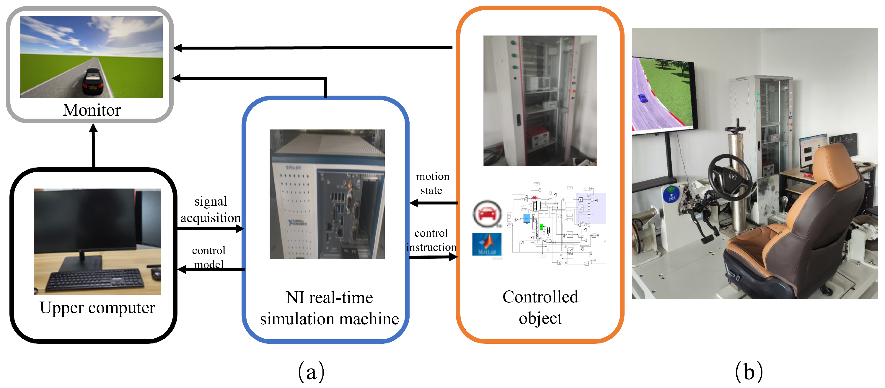
We use a hardware-in-the-loop (HIL) simulation device to validate the above lane-changing trajectory planning algorithm. Unlike the traditional simulation that is only virtualized within the software, the HIL simulation platform can make the simulation results more accurate and convincing by combining real-time hardware and software for real-time simulation [22]. The structure of the HIL simulation platform is illustrated in Figure 7.

Figure 7.
HIL simulation platform: (a) Components of the HIL equipment; (b) Overall setup of the HIL system.
The platform integrates a real-time controller, vehicle dynamics simulation model, traffic environment simulation and algorithm deployment modules to realize a complete closed-loop testing process. The upper processor is equipped with an Intel Core i9-12900K processor (Intel Corporation, Santa Clara, CA, USA) and an NVIDIA RTX 4080 GPU (NVIDIA Corporation, Santa Clara, CA, USA); the real-time controller is used to deploy the trajectory planning and control algorithms; the simulation modeling platform is based on the co-simulation of CarSim and Simulink; the communication interface module simulates the sensor inputs and actuator outputs through the CAN bus and the I/O interfaces; the trajectory planning algorithms are integrated into the Simulink controller in a modular form and run in real time on the HIL platform. The main experimental parameters are summarized in Table 2.

Table 2.
Experiment-related parameters.
5.1. Scenario Configuration
(1) s1: static scenario
When vehicle A is cruising at a certain speed, a stationary obstacle vehicle B suddenly appears in front of the lane where it is located, and it needs to change lanes to avoid it. The speed of vehicle A is set to be 17 m/s, and vehicle B in front of vehicle A is about 45 m. The optimized and improved double-quintic polynomial lane-changing model is simulated with the unoptimized double-quintic polynomial model and the traditional quintic polynomial model for the lane-changing paths.
(2) s2: dynamic scenario
The obstacle vehicles in front of us cannot be all stationary, but are more in dynamic motion, i.e., the obstacle vehicles in front of us have a certain initial velocity and are still decelerating. Set the speed of the vehicle A to 14 m/s; the front obstacle vehicle B is 30 m ahead of the vehicle A; the speed is 12 m/s, and the acceleration of m/s2 is the deceleration.
(3) s3: low coefficient of adhesion pavement scenario
The low traction coefficient road surface will significantly reduce the friction between the tires and the ground, and it is easy for the vehicle to skid and lose control. Therefore, it is necessary to verify the safety and stability in the condition of a low adhesion coefficient environment. Setting the road surface adhesion coefficient to 0.6, the speed of the vehicle 11 m/s, the distance of the obstacle vehicle in front to 40 m, the speed of the vehicle 9 m/s.
5.2. Analysis of Results
(1) s1: static scenario
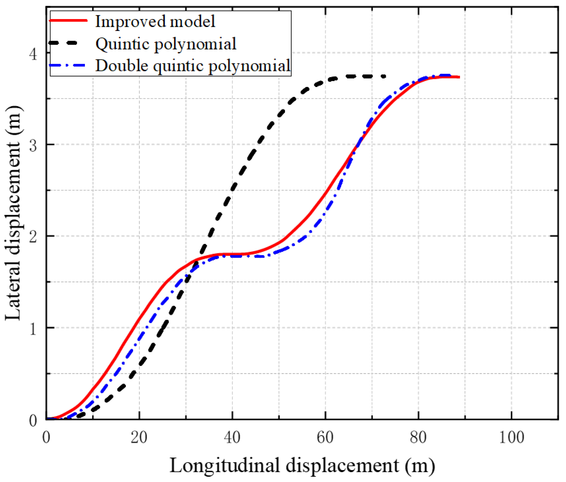
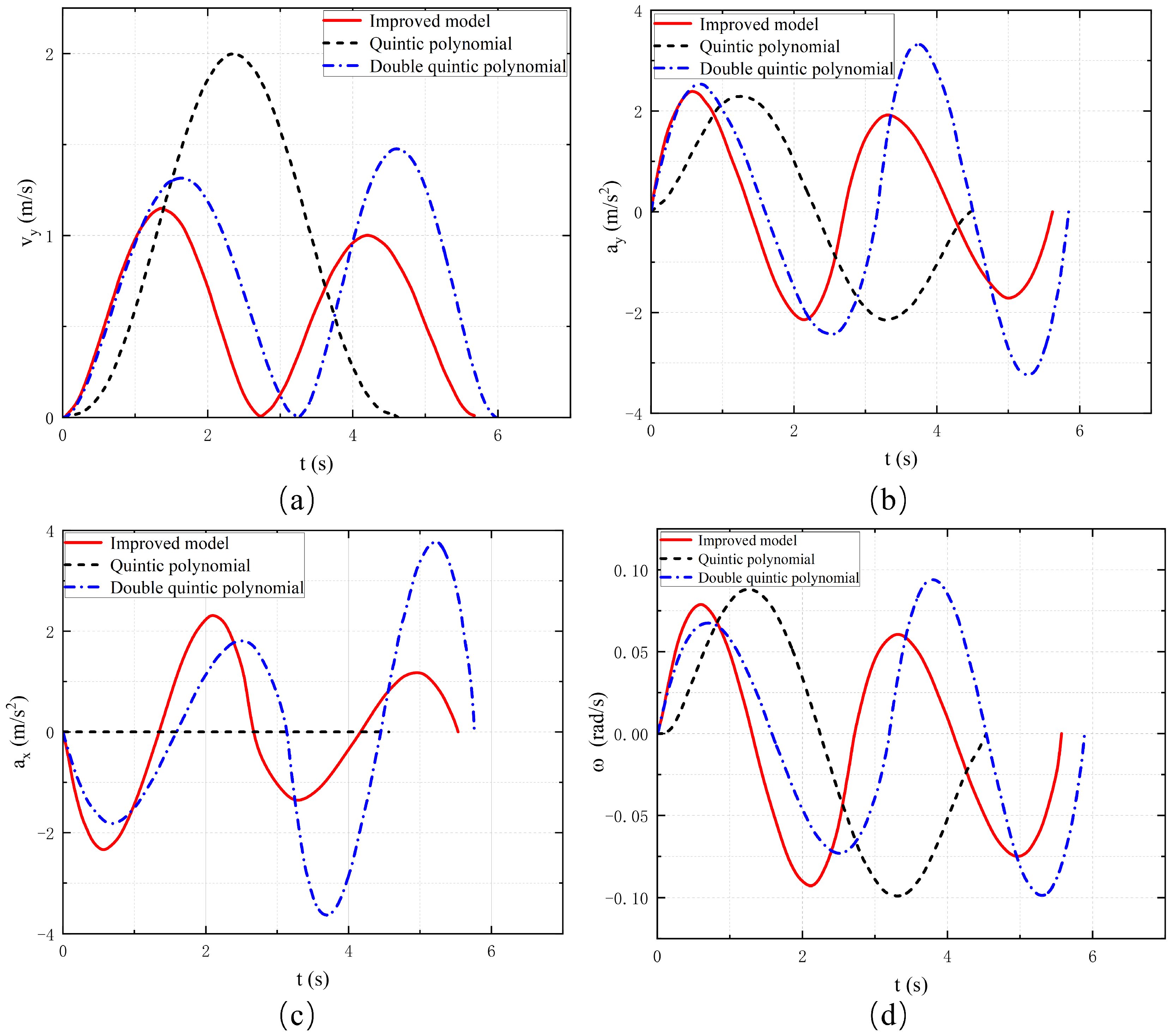
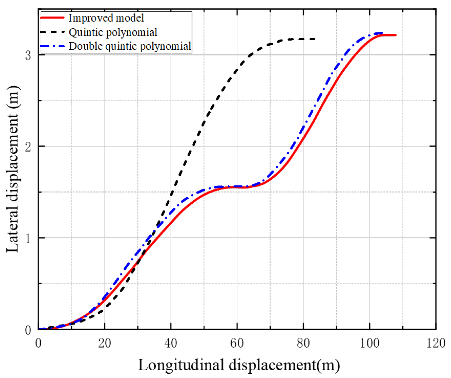
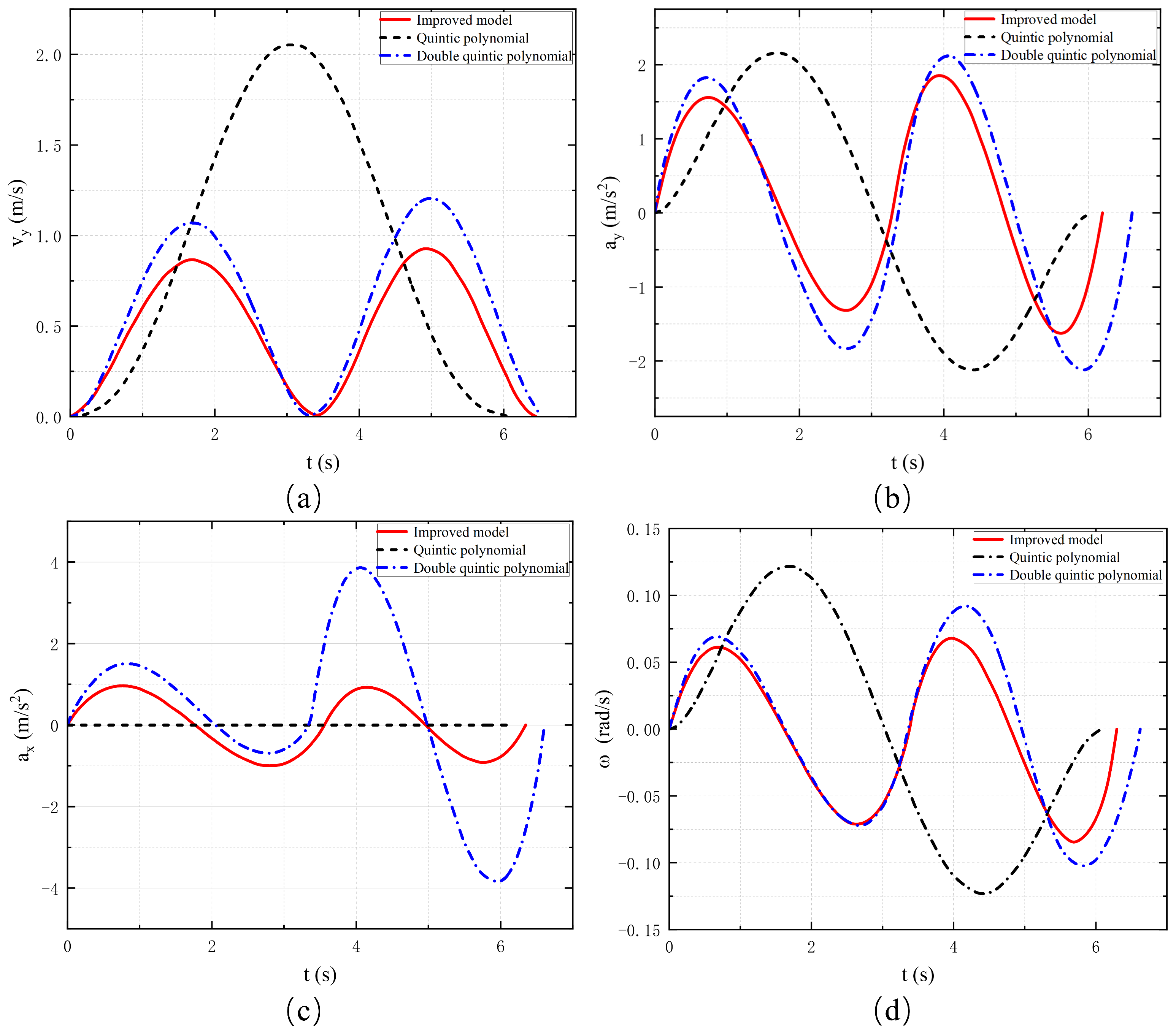
A comparison of planning times across three methods is presented to evaluate computational efficiency. The proposed trajectory planning algorithm, enhanced by the GA-PSO hybrid optimization, achieved the shortest average computation time of 22.3 ms. In contrast, the unimproved version without hybridization took 30.4 ms, and the traditional quintic polynomial method required 25.7 ms on average. All methods satisfy the real-time control cycle requirement (100 ms). The traditional quintic polynomial lane-changing model plans trajectory only via the start and final goal states. It is common to set the longitudinal velocity constant and utilize a larger transverse velocity and transverse acceleration as a way to avoid collision with the vehicle B during the lane-changing process. Figure 8 and Figure 9 show that the time required for lane-changing is shorter and the longitudinal displacement is smaller than that of the two quintic polynomials. However, the vehicle moves violently in the transverse direction, especially in Figure 9a, which shows that its transverse velocity is much larger than that of the other two models. Therefore, the traditional quintic polynomial model is less stable and comfortable.
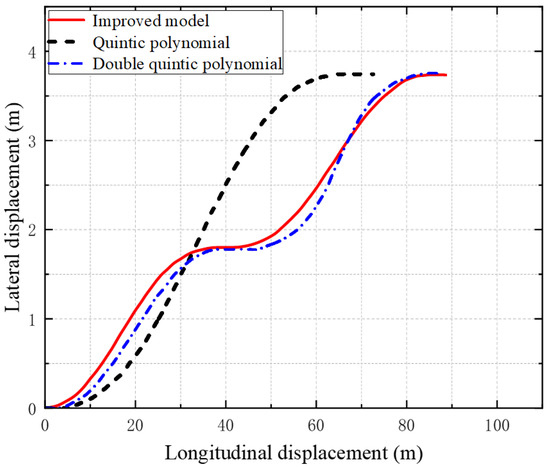
Figure 8.
Planning trajectories for models.
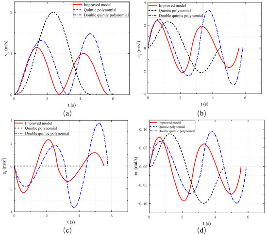
Figure 9.
(a) Lateral velocity. (b) Lateral acceleration. (c) Longitudinal acceleration. (d) Yaw rate.
The double-quintic polynomial lane-changing model separates the lane-changing process into two phases by adding transition states. The vehicle only needs to move a certain distance laterally in the first half of the process to avoid the obstacle vehicle in front of it. Since the vehicle in front is stationary and will not move forward, the lane-changing vehicle takes a deceleration in the longitudinal direction to reserve more time for lane-changing in the first phase, and the longitudinal acceleration is shown in Figure 9c. Even so, the front vehicle is stationary compared to the front vehicle with a certain speed; the lane-changing time in the first phase is still a little shorter, so the vehicle’s transverse velocity and transverse acceleration are also slightly larger, and the main vehicle’s transverse motion parameters are shown in Figure 9a,b. After the lane-changing vehicle passes through the staging position, the remaining second phase of lane-changing is equivalent to the barrier-free lane-changing, and there is no obstacle avoidance task in this phase, so it only needs to travel to the final target position. As can be seen through Figure 9a,b,d, the vehicle’s transverse angular velocity as well as the values of lateral velocity and lateral acceleration are smaller in this phase, in which the stability of the lane-changing vehicle and the passenger’s ride comfort are a bit better. In particular, our proposed optimized double-quintic polynomial commutation model not only satisfies the constraints in terms of velocity, acceleration, and angular velocity of the pendulum, but also has smaller fluctuations in the range of values compared to the unoptimized double-quintic polynomial model. Therefore, the optimized model is more stable and comfortable.
(2) s2: dynamic scenario
In a second test under a dynamic environment, our proposed hybrid algorithm achieved an average planning time of 35.6 ms, compared to 49.5 ms without the hybrid improvement and 45.3 ms using the traditional quintic polynomial method. All three methods meet the real-time requirement of the control cycle. The planned trajectories and the dynamic response results under different methods are shown in Figure 10 and Figure 11, respectively. In Figure 11, the peak value of the transverse velocity profile of the improved double quintuple permutation trajectory is lower than 1.0 m/s. Compared with the other two models, the improved permutation model trajectory satisfies the constraints in terms of transverse acceleration and longitudinal acceleration as well as transverse pendulum angular velocity, and the range of fluctuation of the values is lower compared with the other two models, so that the optimized and improved double quintuple polynomial permutation model is better in terms of stability and comfort. Therefore, the optimized and improved double-quintic polynomial commutation model is more stable and comfortable.
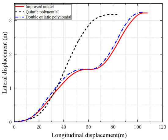
Figure 10.
Planning trajectories for models.
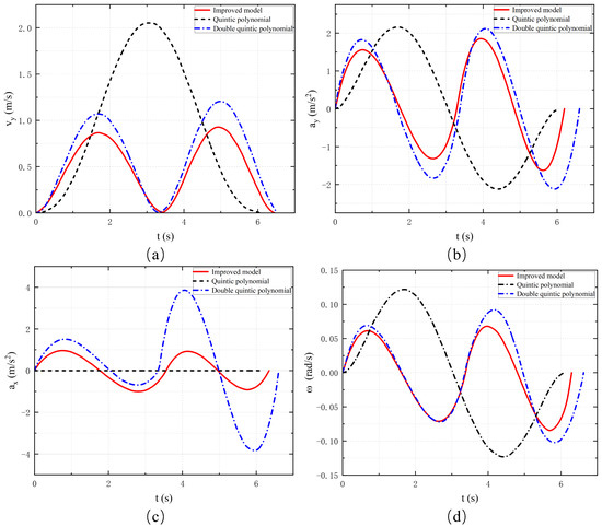
Figure 11.
(a) Lateral velocity. (b) Lateral acceleration. (c) Longitudinal acceleration. (d) Yaw rate.
(3) s3: low coefficient of adhesion pavement scenario
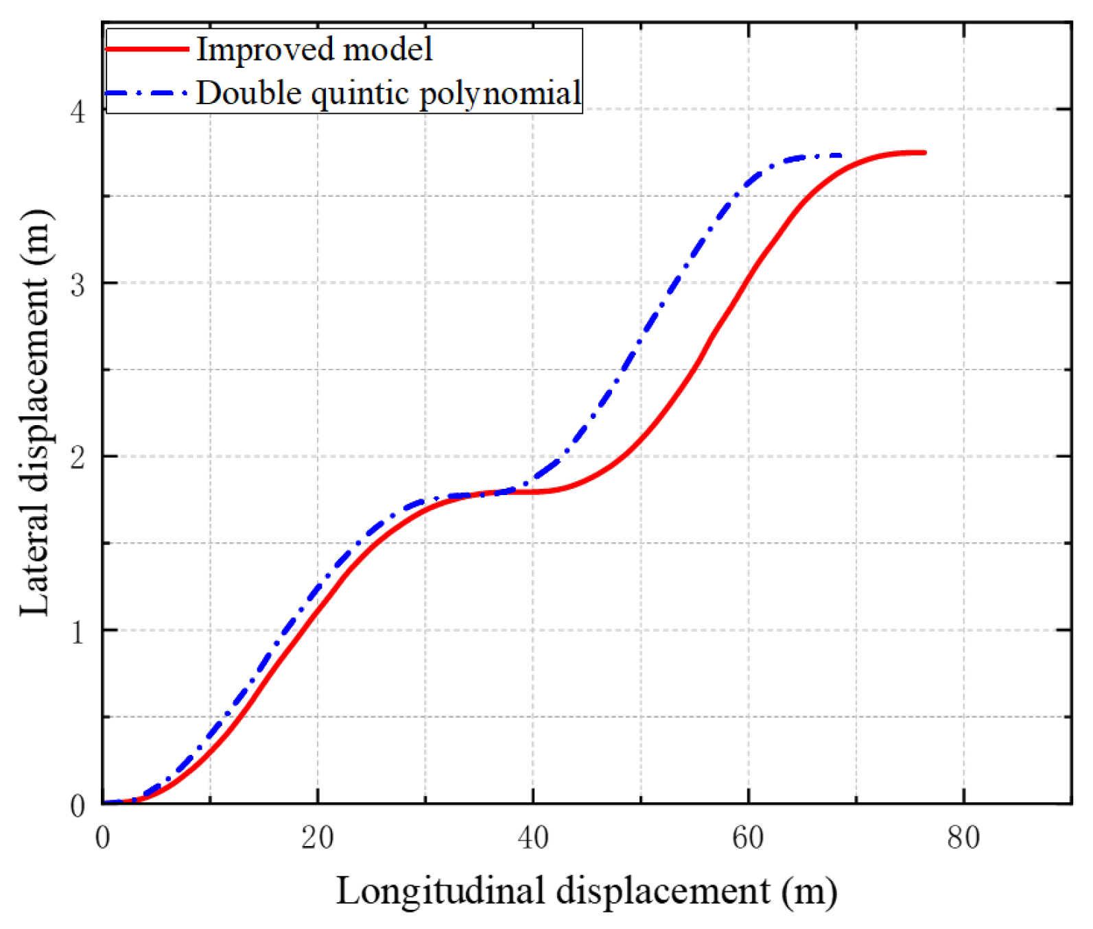
In the third group of experiments conducted under low-adhesion road conditions, the proposed hybrid planning algorithm achieved an average computation time of 27.3 ms, compared to 36.8 ms for the non-hybrid version. Both algorithms met the real-time requirements of the control cycle. Based on Figure 12 and Figure 13, it can be seen that the optimized and improved lane-changing model, compared with the unoptimized model, improves the performance in many aspects, such as transverse velocity, transverse acceleration, and transverse angular velocity. Not only do the values all satisfy the constraints, but also the range of numerical fluctuations is a bit smaller, so the improved model is suitable for roads with low coefficient of adhesion.
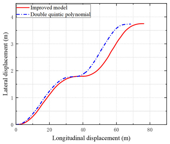
Figure 12.
Planning trajectories for models.
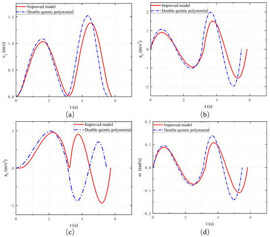
Figure 13.
(a) Lateral velocity (b) Lateral acceleration. (c) Longitudinal acceleration. (d) Yaw rate.
6. Conclusions and Future Work
A lane-changing trajectory planning method via improved quintic polynomials for intelligent cars is proposed. For the unidirectional two-lane scenario, first, by analyzing the critical collision state between the two cars, and at the same time, considering the state of the two cars to determine the transit position, the lane-changing process is segmented into the front and rear parts, and the quintic polynomials are utilized for trajectory planning, respectively. Then, according to the different characteristics of the lane-changing paths in the front and rear segments, a multi-objective optimization function with different weight coefficients is established. A safe and comfortable lane-changing trajectory is achieved through the improved particle swarm optimization algorithm. Finally, the robustness and adaptability of the algorithm in different environments are verified through hardware-in-the-loop simulation tests. The results show that the lane-changing trajectories planned by the proposed model have significant advantages in terms of safety, comfort and real-time performance, and have good suitability in the face of static and dynamic obstacle vehicles, as well as on low-traction surfaces.
Due to limitations in experimental conditions, the scenarios selected in this paper are relatively simple and have not been systematically compared with other advanced trajectory planning methods. To further improve the adaptability and practicality of the proposed model, we plan to introduce predictive interaction models, such as the Intelligent Driver Model (IDM) or game-theoretic planning, to more effectively handle the uncertain behaviors of surrounding vehicles. The decision-making system will be based on the prediction information of surrounding vehicles and combined with a lane-change safety distance model to determine whether the conditions for a safe lane change are met. Once the feasibility and risk assessment criteria are satisfied, the lane-change command will be issued to the planning system. In future work, we also intend to extend the current highway-focused setting to urban or mixed-traffic environments, and conduct side-by-side comparisons with other state-of-the-art trajectory planning algorithms to more comprehensively evaluate the effectiveness of the proposed method.
Author Contributions
Conceptualization, Y.Z. and L.C.; methodology, Y.Z.; software, N.L.; validation, Y.Z., L.C. and N.L.; formal analysis, Y.Z.; investigation, Y.Z.; resources, Y.Z., L.C. and N.L.; data curation, Y.Z.; writing—original draft preparation, Y.Z.; writing—review and editing, Y.Z. and L.C.; supervision, L.C.; project administration, L.C. All authors have read and agreed to the published version of the manuscript.
Funding
This research received no external funding.
Data Availability Statement
The original contributions presented in this study are included in the article. Further inquiries can be directed to the corresponding author.
Conflicts of Interest
The authors declare no conflict of interest.
References
- Di Lillo, L.; Gode, T.; Zhou, X.; Atzei, M.; Chen, R.; Victor, T. Comparative safety performance of autonomous-and human drivers: A real-world case study of the Waymo Driver. Heliyon 2024, 10, e34379. [Google Scholar] [CrossRef] [PubMed]
- Abdel-Aty, M.; Ding, S. A matched case-control analysis of autonomous vs human-driven vehicle accidents. Nat. Commun. 2024, 15, 4931. [Google Scholar] [CrossRef] [PubMed]
- Montanaro, U.; Dixit, S.; Fallah, S.; Dianati, M.; Stevens, A.; Oxtoby, D.; Mouzakitis, A. Towards connected autonomous driving: Review of use-cases. Veh. Syst. Dyn. 2019, 57, 779–814. [Google Scholar] [CrossRef]
- Wang, H.; Xu, S.; Deng, L. Automatic lane-changing decision based on single-step dynamic game with incomplete information and collision-free path planning. Actuators 2021, 10, 173. [Google Scholar] [CrossRef]
- Schütt, B.; Ransiek, J.; Braun, T.; Sax, E. 1001 ways of scenario generation for testing of self-driving cars: A survey. In Proceedings of the 2023 IEEE Intelligent Vehicles Symposium (IV), Anchorage, AK, USA, 4–7 June 2023; IEEE: Piscataway, NJ, USA, 2023; pp. 1–8. [Google Scholar]
- Chen, S.; Hu, X.; Zhao, J.; Wang, R.; Qiao, M. A review of decision-making and planning for autonomous vehicles in intersection environments. World Electr. Veh. J. 2024, 15, 99. [Google Scholar] [CrossRef]
- Paden, B.; Čáp, M.; Yong, S.Z.; Yershov, D.; Frazzoli, E. A survey of motion planning and control techniques for self-driving urban vehicles. IEEE Trans. Intell. Veh. 2016, 1, 33–55. [Google Scholar] [CrossRef]
- Zeng, D.; Yu, Z.; Xiong, L.; Zhao, J.; Zhang, P.; Li, Y.; Xia, L.; Wei, Y.; Li, Z.; Fu, Z. Driving-behavior-oriented trajectory planning for autonomous vehicle driving on urban structural road. Proc. Inst. Mech. Eng. Part D J. Automob. Eng. 2021, 235, 975–995. [Google Scholar] [CrossRef]
- Yu, L.; Wang, X.; Hou, Z.; Du, Z.; Zeng, Y.; Mu, Z. Path planning optimization for driverless vehicle in parallel parking integrating radial basis function neural network. Appl. Sci. 2021, 11, 8178. [Google Scholar] [CrossRef]
- Wang, H.; Huang, Y.; Khajepour, A.; Zhang, Y.; Rasekhipour, Y.; Cao, D. Crash Mitigation in Motion Planning for Autonomous Vehicles; IEEE: Piscataway, NJ, USA, 2019; Volume 20, pp. 3313–3323. [Google Scholar]
- Sharma, O.; Sahoo, N.C.; Puhan, N.B. Recent advances in motion and behavior planning techniques for software architecture of autonomous vehicles: A state-of-the-art survey. Eng. Appl. Artif. Intell. 2021, 101, 104211. [Google Scholar] [CrossRef]
- Li, D.; Yin, W.; Wong, W.E.; Jian, M.; Chau, M. Quality-oriented hybrid path planning based on A* and Q-learning for unmanned aerial vehicle. IEEE Access 2021, 10, 7664–7674. [Google Scholar] [CrossRef]
- Nilsson, J.; Brännström, M.; Coelingh, E.; Fredriksson, J. Lane-change maneuvers for automated vehicles. IEEE Trans. Intell. Transp. Syst. 2017, 18, 1087–1096. [Google Scholar] [CrossRef]
- Guo, L.; Ge, P.S.; Yue, M.; Zhao, Y.B. Lane changing trajectory planning and tracking controller design for intelligent vehicle running on curved road. Math. Probl. Eng. 2014, 2014, 478573. [Google Scholar] [CrossRef]
- Xu, L.H.; Hu, S.G.; Wu, S.; Luo, Q. Overtaking model for two-lane highway considering vehicle running characteristics. J. South China Univ. Technol. Nat. Sci. Ed. 2015, 43, 7–14. [Google Scholar]
- Yuan, J.; Zheng, L.; Liu, Y. A Real-Time Trajectory Planning Method for Autonomous Vehicles Based on Fifth-Order Polynomial Optimization. In Proceedings of the 2021 IEEE International Conference on Intelligent Transportation Systems (ITSC), Indianapolis, IN, USA, 19–22 September 2021. [Google Scholar]
- Gu, J.; Zhang, H.; Fang, Y. Exploring pollution control in transboundary watersheds under the perspective of ecological compensation based on aggregate game. Environ. Sci. Pollut. Res. 2024, 31, 13981–14002. [Google Scholar] [CrossRef] [PubMed]
- Hou, K.; Zheng, F.; Liu, X.; Fan, Z. Cooperative vehicle platoon control considering longitudinal and lane-changing dynamics. Transp. A Transp. Sci. 2024, 20, 2182143. [Google Scholar] [CrossRef]
- Ye, X.m.; Chen, B.; Fan, Q. A Fuzzy-Hybrid Algorithm for Solving Multi-objective War-time Transport Path Optimization. In Proceedings of the 2009 Second International Conference on Computer and Electrical Engineering, Dubai, United Arab Emirates, 28–30 December 2009; IEEE: Piscataway, NJ, USA, 2009; Volume 2, pp. 134–138. [Google Scholar]
- Li, Q.; Ma, Q.; Weng, X. Dynamic path planning for mobile robots based on artificial potential field enhanced improved multiobjective snake optimization (APF-IMOSO). J. Field Robot. 2024, 41, 1843–1863. [Google Scholar] [CrossRef]
- GB/T 13441.1-2007; Standards of the People’s Republic of China. Mechanical Vibration and Shock—Evaluation of Human Exposure to Whole-Body Vibration. China Quality Inspection Press: Beijing, China, 2007.
- Weng, X.; Liu, F.; Mai, J.; Zhou, S.; Feng, S. Trajectory planning strategy for obstacle avoidance based on D-APF. J. Braz. Soc. Mech. Sci. Eng. 2025, 47, 85. [Google Scholar] [CrossRef]
Disclaimer/Publisher’s Note: The statements, opinions and data contained in all publications are solely those of the individual author(s) and contributor(s) and not of MDPI and/or the editor(s). MDPI and/or the editor(s) disclaim responsibility for any injury to people or property resulting from any ideas, methods, instructions or products referred to in the content. |
© 2025 by the authors. Published by MDPI on behalf of the World Electric Vehicle Association. Licensee MDPI, Basel, Switzerland. This article is an open access article distributed under the terms and conditions of the Creative Commons Attribution (CC BY) license (https://creativecommons.org/licenses/by/4.0/).

