Research on Trajectory Prediction Based on Front Vehicle Sideslip Recognition

Abstract

In order to solve the problem of emergency collision avoidance of autonomous vehicles when the front vehicle is unstable and sliding under high-speed conditions, a research method for the state recognition of the front side-skid vehicle and the trajectory prediction of the front side-skid vehicle was proposed. By extracting the key features of the vehicle in front of the vehicle in danger of sliding to build a skidding recognition model of the vehicle in front, a skidding recognition strategy of the vehicle in front was designed based on the extracted skidding feature indexes to judge the skidding state of the vehicle in front. The state quantity of the sliding vehicle in front is selected, and the constant rotation rate and acceleration model (CTRA) is established to predict the trajectory of the sliding vehicle in front in a short time. Considering the simplified assumptions of the model and the noise in the process of sensor perception information, the Unscented Kalman Filter (UKF) is used to deal with the uncertainty in the trajectory prediction process, the possible position and covariance of the front sideslipping vehicle are calculated, and the possible future area of the front sideslipping vehicle is estimated under the condition of a probability of 0.9. Through the established Carsim and Simulink co-simulation platform, the effectiveness of the front vehicle skidding state recognition strategy and the accuracy of the trajectory prediction of the sliding vehicle are verified under the condition of high speed and low attachment.

1. Preamble

Vehicle speed on the highway is very high; if a sudden destabilization occurs, whether for the car or the surrounding vehicles, this is extremely dangerous, and when serious, it easily leads to major traffic accidents. It is of great significance to carry out research on predicting the trajectory of skidding vehicles under the destabilizing condition of the front vehicle to improve driving safety.

Surrounding vehicle behavior recognition methods are divided into two types: logical rules and machine learning [1,2]. The method based on logical rules is to use expert knowledge to set rules, and according to the rules, to determine or infer the behavior of the vehicle. The advantage of this method is that it has strong interpretability, but its disadvantages are that it requires a large amount of high-quality data, the applicability of the rules is poor, and it cannot be well applied to different scenarios and environments [3,4]. At present, the more commonly used vehicle behavior recognition method is based on a machine learning method, which involves using data to train a recognition model to identify vehicle behavior. The advantage of this method is that it has a strong learning ability and can automatically learn the characteristics and laws of vehicle behavior from the data, but its disadvantage is that the construction of the model depends on the quality and quantity of the data set, and the interpretability of the model is very poor. Zhu [5] proposed a driving behavior recognition method using a support vector machine (SVM) in 2017. This method takes the distance difference and speed difference between the target vehicle and the surrounding vehicle, as well as the speed and position of the target vehicle, as feature vectors. The final results show that the designed method has high recognition accuracy.

The vehicle center-of-mass lateral deflection angle and transverse swing angle can reflect the vehicle sideslip state. At present, local scholars and scholars abroad have designed various methods for estimating the center-of-mass lateral deviation angle based on vehicle kinematics or dynamics models. Chung [6] proposed a method for estimating the vehicle sideslip state using an ESP sensor and verified the performance and effectiveness of the proposed estimation and compensation algorithms through vehicle tests. Ma Biao [7] proposed a steering torque-based method for estimating the center-of-mass lateral deflection angle and designed an extended Kalman filter. Finally, the method is demonstrated to have better accuracy and faster response compared to the steering angle-based method through simulation and vehicle testing. Enming Lai et al. [8] built a center-of-mass lateral deflection estimator based on a vehicle two-degree-of-freedom dynamics model, which consists of two algorithms: the Kalman filter algorithm and the dynamics integration algorithm. Different algorithms are switched according to the magnitude of the center-of-mass lateral declination to estimate the vehicle’s center-of-mass lateral declination. Most of the above studies on the recognition of surrounding vehicle behavior are based on the information perceived by the auto-vehicle to recognize the behavior of the surrounding non-stable vehicles, and the recognition of the behavior of the vehicle in front of the vehicle in high-speed unstable working conditions is not considered.

Regarding vehicle trajectory prediction research, Shirazi [9] summarized behavioral prediction methods at intersections based on drivers’ actions, and Mozaffari [10] reviewed deep learning-based vehicle behavior analysis methods in 2019. Ruifeng Zhang [11] predicted vehicle trajectories based on vehicle-to-vehicle communication and KF to prevent collisions with obstacles. Lefkopoulos [12] designed the Interactive Multi-Model Kalman Filter (IMM-KF) considering interaction-related factors to predict the future trajectories of a vehicle using a physical model-based approach. The method, while considering uncertainty in trajectory prediction, is only applicable to linear models. Okamoto [13] captured the intentions of drivers of other vehicles through a random forest classifier and combined it with a sequential Monte Carlo method to compute their possible future trajectories and potential threats to their own vehicles. Yijing Wang [14] predicted the motion of other traffic participants using the Monte Carlo method and combined it with a model predictive control algorithm to optimize the reference trajectory based on the current state of the self-driving vehicle, thus improving the safety of the self-driving vehicle. The physical model-based trajectory prediction method of the above study consumes less computational resources, but due to the fact that the physical model of the traffic vehicle changes at any time, it may cause obvious prediction errors during model selection and switching.

In summary, the problems of the difficulty in identifying the behavior of front destabilized vehicles under high-speed conditions and the poor trajectory prediction accuracy of sidesliding vehicles using physical models are addressed. It is proposed to extract four sideslip feature indicators to design the front vehicle sideslip state recognition strategy and establish the constant turn rate and acceleration model to predict the front trajectory in a short period of time to guarantee the driving safety of intelligent vehicles.

2. Introduction

2.1. Characterization of Forward Vehicle Skidding

Sideslip Scene

For vehicles in the process of high-speed driving, a common sideslip trajectory is shown in Figure 1. If the vehicle is in front of the sideslip, as shown in sideslip trajectory 2, the sideslip vehicle is only in its lane slip driving and does not slide into other lanes. This kind of skid is called “ordinary skid”.

However, if the vehicle is in front of the vehicle skids as shown in skid trajectory 1 or 3, the vehicle skidding in this case may suddenly slide into other lanes, forcing other vehicles to brake or take evasive action. In order to distinguish it from ordinary skidding, this type of skidding is called “dangerous skidding” [15].

After the occurrence of dangerous skidding, the trajectory of vehicles is usually in the shape of an arc. According to the different characteristics of the sideslip trajectory, this can be divided into two kinds of dangerous sideslips: the first sideslip situation is that the vehicle slides out of its lane directly from one side of the lane line, such as sideslip trajectory 3 in Figure 1; the second sideslip situation is that the vehicle firstly gets closer and closer to one side of the lane line, but it does not slide out of the lane from this side, and instead rushes out of the lane from the other side, such as in sideslip trajectory 1 in Figure 1, which characterizes this dangerous sideslip in depth.

2.2. Sideslip Feature Extraction

The relative position of the self-driving vehicle to the vehicle in front of it is shown in Figure 2. The exact position of the self-driving vehicle itself $(X_S,Y_s)$, as well as vehicle speed $V_S$ and traverse angle ${\phi }_s$ information, can be accurately obtained from autonomous vehicle positioning systems (e.g., GPS) and inertial sensors (IMU). The relative speed, direction, and distance between the vehicle in front and the self-driving vehicle can be obtained from the sensing systems in the self-driving vehicle, such as cameras and radar. Based on the information obtained above, the speed and position of the front vehicle can be estimated as follows:

$$\{\begin{array}{c}{v}_o=v_s+v_c\\ X_o=X_s+Lcos({\alpha }_S+{\phi }_S)\\ Y_o=Y_s+L\sin ({\alpha }_S+{\phi }_S)\end{array}$$

(1)

where $v_0$ is the speed of the vehicle ahead and $\left(X_0,Y_0\right)$ is the position of the vehicle ahead.

In order to quantitatively characterize these sideslip features of the vehicle in front, the centrifugal acceleration of the vehicle in front is first known to determine the existence of extreme values, which is the first indicator to characterize the sideslip features; in addition to this, in order to assess whether the vehicle in front has the risk of sliding out of the lane in which it is located very quickly, the other three main characteristic indicators are considered: the distance between the edge of the vehicle in front and the lane line, the sideways velocity with respect to the lane line, and the time it takes for the edge to reach the lane line.

(1)

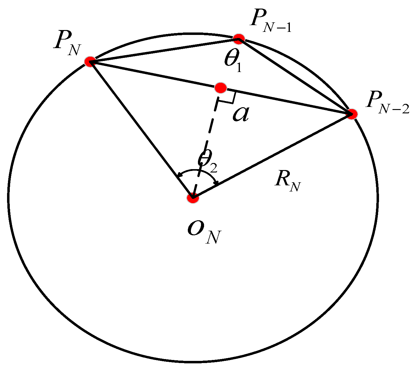
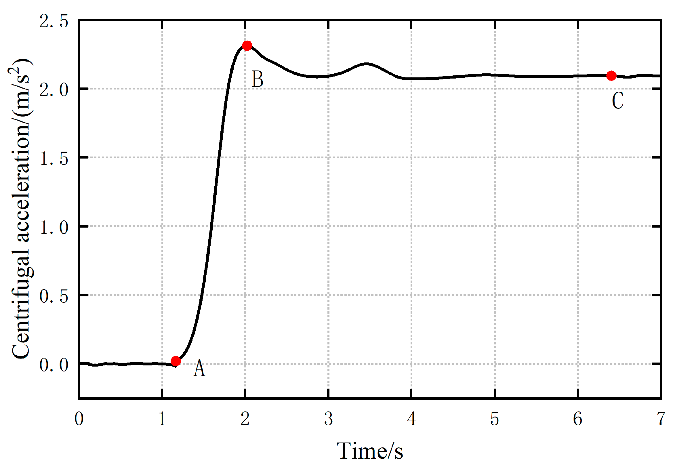
Centrifugal acceleration

As shown in Figure 3, the points $P_{N-2},P_{N-1},P_N$ represent the trajectories of the front car at three consecutive moments $N-2,N-1,N$, where the corresponding position coordinates are $(X_N,Y_N)$, $\left(X_{N-1},Y_{N-1}\right)$, and $(X_{N-2},Y_{N-2})$, respectively. Using the distance between the two points, formulas can be used to calculate the length of the three sides of the triangle, $P_{N-2},P_{N-1}, \mathrm{and} P_N$; the specific expressions are shown below:

$$S_{N-2,N-1}=\sqrt{{(X_{N-1}-X_{N-2})}^2+{(Y_{N-1}-Y_{N-2})}^2}$$

(2)

$$S_{N-1,N}=\sqrt{{(X_N-X_{N-1})}^2+{(Y_N-Y_{N-1})}^2}$$

(3)

$$S_{N-2,N}=\sqrt{{(X_N-X_{N-2})}^2+{(Y_N-Y_{N-2})}^2}$$

(4)

In a triangle with $P_{N-2}, P_{N-1}, \mathrm{and} P_N$, the angle of intersection, can be calculated from the cosine theorem with the following expression:

$${\theta }_1=\arccos ({\displaystyle \frac{S_{N-2,N-1}^2+S_{N-1,N}^2-S_{N-2,N}^2}{2S_{N-2,N-1}{S}_{N-1,N}}})$$

(5)

We assume that the three historical trajectory points $P_{N-2},P_{N-1},P_N$ of the vehicle are on a circle with a center and radius $O_N$. Using the properties of circles, it is easy to conclude that $=2\left(\pi -{\theta }_1\right)$, where ${\theta }_2$ is the angle of the center of the circle and $P_{N-2},P_{N-1}$ is the angle subtended by the segment. A vertical line $P_{N-2},P_{N-1}$ is made through the center $O_N$ of the circle to the segment, with the foot $a$ of the line at the point. In a triangle $O_{N}a{P}_{N-2}$, the radius $R_{N }$ of the circle is given by the following sine theorem:

$$R_N={\displaystyle \frac{\frac{1}{2}{S}_{N-2,N}}{\sin (\frac{{\theta }_2}{2})}}$$

(6)

After obtaining the radius $R_N$ of the curvature of the traveling trajectory of the vehicle in front at the time $N$ through expression (6), the centrifugal acceleration of the vehicle in front at the time $N$ is estimated by combining it with the speed $a_N$ of the vehicle in front at that time, and the specific expression is as follows:

$$a_N={\displaystyle \frac{v_N^2}{R_N}}$$

(7)

(2)

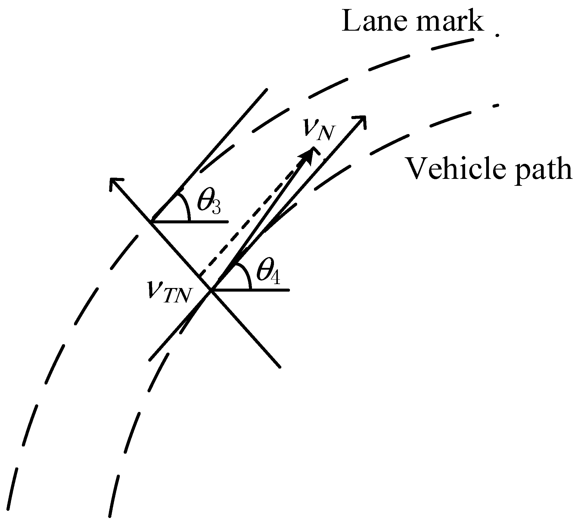
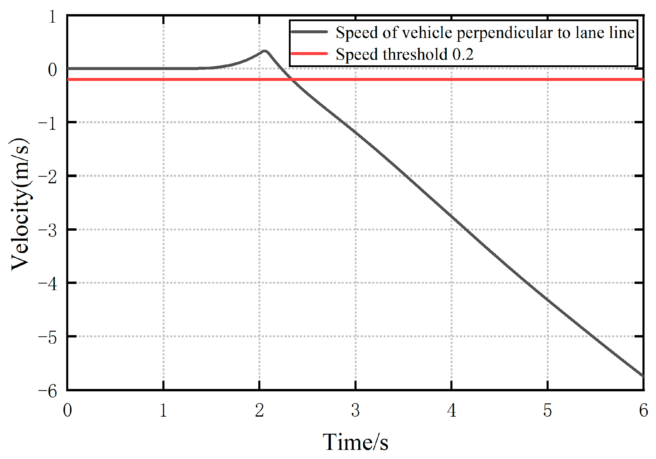
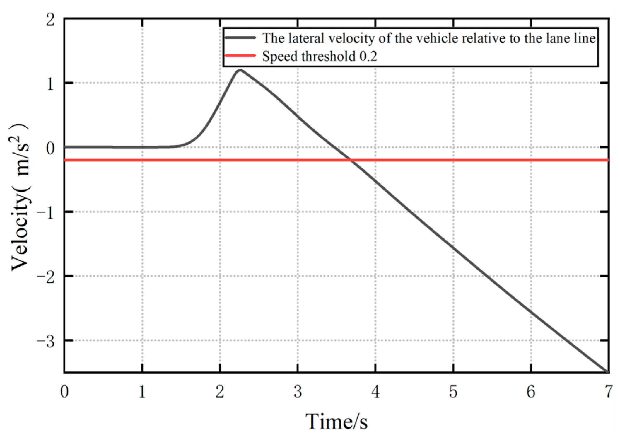
Lateral speed of the vehicle ahead relative to the lane line

Figure 4 illustrates the relative positional relationship between the trajectory of the vehicle ahead and the lane line. The self-driving vehicle is able to capture information about the lane lines through its visual perception system. Here, ${\theta }_3$ denotes the tangential direction of the lane line, and ${\theta }_4$ is the direction of speed of the vehicle in front. According to the simple trigonometric relationship, it is easy to derive the lateral speed $v_{TN }$ of the front vehicle relative to the direction of the lane line at the time $N$:

$$v_{TN}=v_N\sin ({\theta }_4-{\theta }_3)$$

(8)

(3)

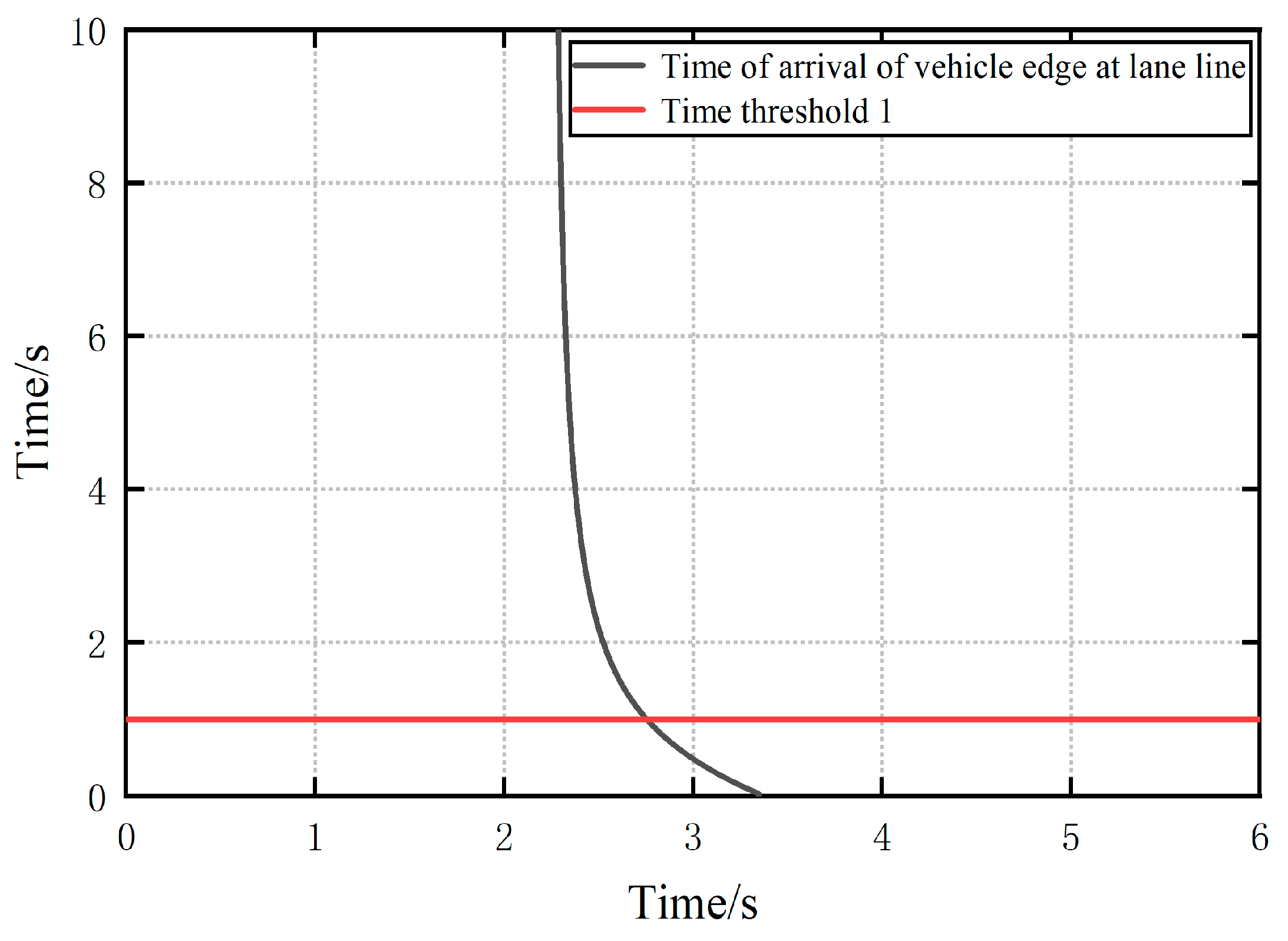
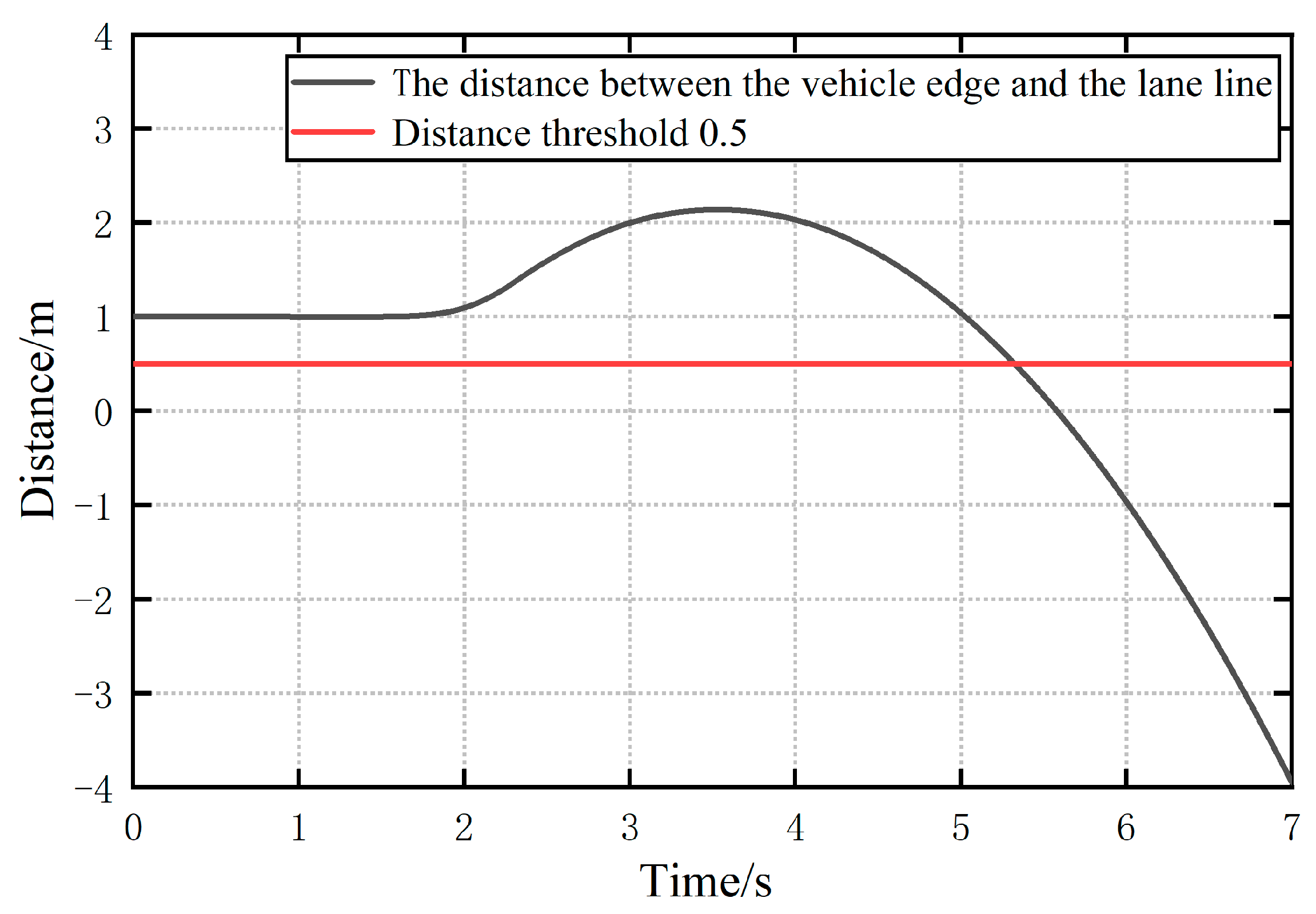
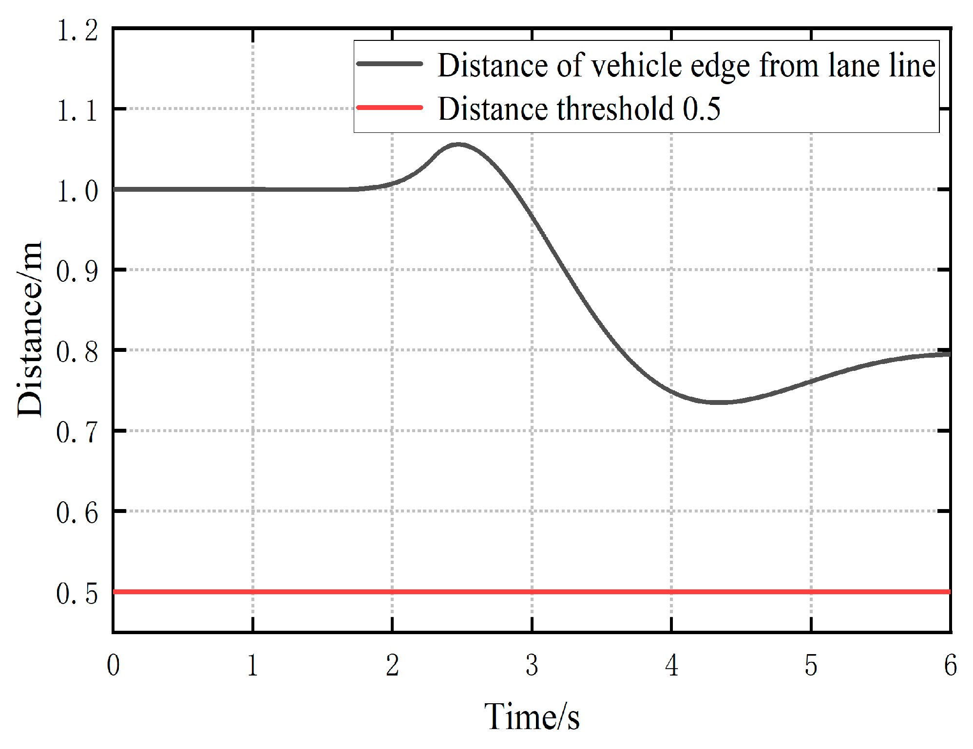
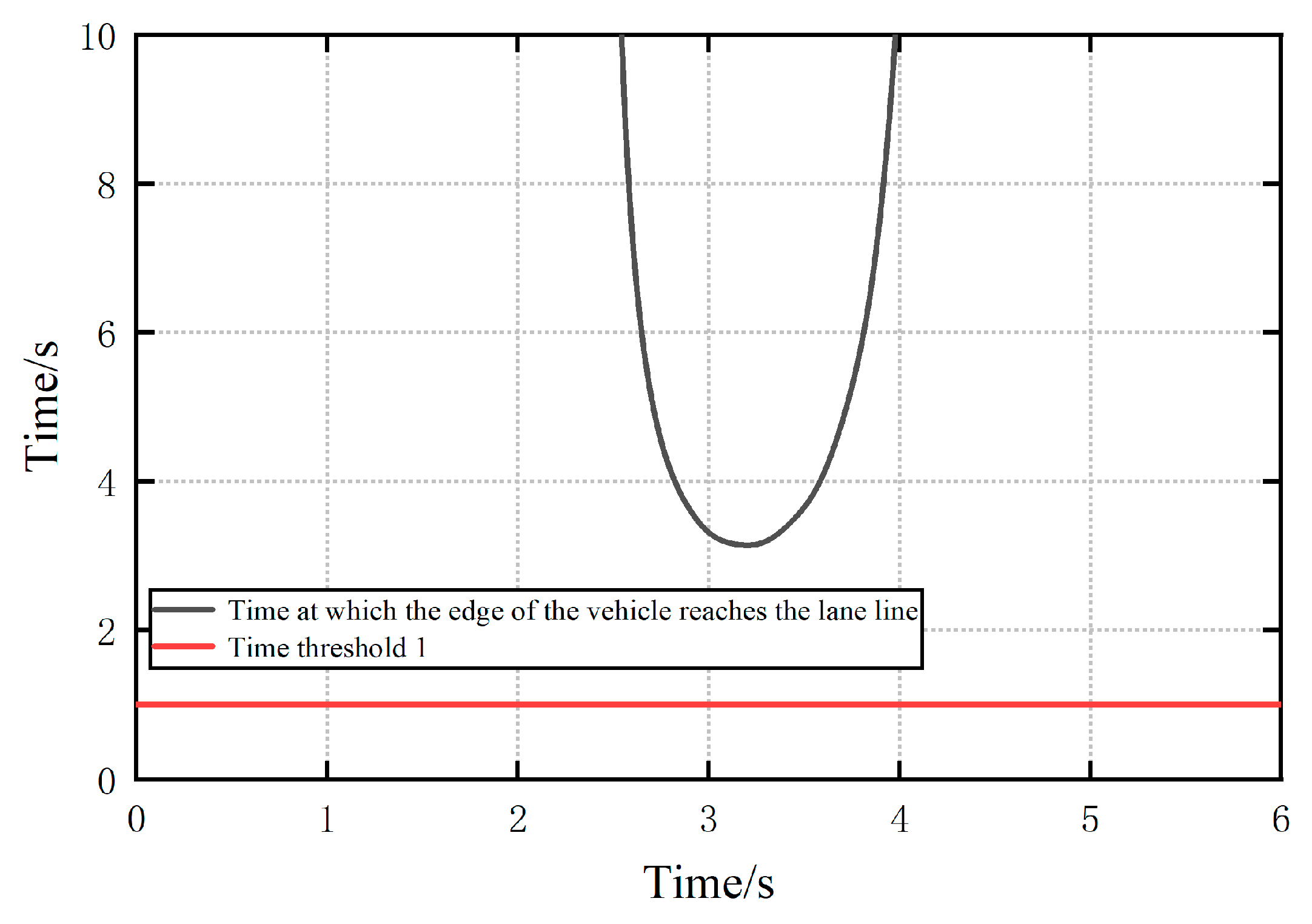
Time of arrival of the edge of the front vehicle at the lane line

The automatic driving vehicle sensing system can obtain the distance between the edge of the front vehicle and the lane line, assuming that the lateral velocity of the front vehicle relative to the lane line remains basically unchanged in a short period of time; combined with Equation (8), the following expression can be used to calculate the time when the edge of the vehicle in front of the time arrives at the lane line:

$$t_N={\displaystyle \frac{l}{v_{TN}}}$$

(9)

2.3. Strategy for Recognizing the Sideslip State of the Front Vehicle

A front vehicle sideslip state recognition strategy is designed in combination with feature indicators and includes the determination criteria of whether the front vehicle has sideslip characteristics. The specific flowchart of the front vehicle sideslip state recognition strategy is shown in Figure 5.

(a)

Calculate the centrifugal acceleration of the vehicle in front of you at the moment of time $N$ based on the sensed information.

(b)

Compare the historical centrifugal accelerations from the moment $a_1$ to the moment $a_N$ and determine if there is an extreme value. If there is no extreme value, then the moment $N=N+1$; then, go back to step a and continue to calculate the centrifugal acceleration at the next moment. If there is an extreme value in the historical centrifugal acceleration, mark the extreme point as k and proceed to step c.

(c)

Analyze the distance between the edge of the front car and the lane line on one side of the car during the period from moment k to moment $N$. If it is gradually decreasing, go to step d; otherwise, go to step f.

(d)

Calculate three metrics used at time N to characterize whether the vehicle in front will quickly slide out of the lane it is in: the distance between the edge of the vehicle in front and the lane line, the lateral speed relative to the lane line, and the time for the edge to reach the lane line. If one or more of these three metrics do not reach the set threshold, then go to step e; conversely, if all of them reach the set threshold, then go to step i.

(e)

Calculate the centrifugal acceleration of the front vehicle at the next moment $N=N+1$. If it does not exceed the centrifugal acceleration at the k-moment, go back to step c for further judgment; conversely, at moment $N=N+1$, go back to step a and continue to calculate the centrifugal acceleration at the next moment.

(f)

Analyze the distance between the edge of the front car and the lane line on the other side of the car during the period from moment k to the next moment. If it is gradually shortened, then go to the next step g; conversely, for moment $N=N+1$, go back to step a, and continue to calculate the centrifugal acceleration at the next moment.

(g)

As in step d, calculate the three indicators used to characterize whether the vehicle in front will slide out of its lane quickly at the designated time. If one or more of the three indicators do not reach the set threshold, then go to the next step h; conversely, if all of them reach the set threshold, then go to step i.

(h)

Calculate the centrifugal acceleration of the front vehicle at the next moment $N=N+1$. If it does not exceed the centrifugal acceleration at the k-moment, go back to step f for further judgment; conversely, for the moment $N=N+1$, go back to step a and continue to calculate the centrifugal acceleration at the next moment.

(i)

This only means that the vehicle in front of you may be skidding, which is further determined by the turn signal information of the vehicle in front of you. If the vehicle in front of you does not have turn signals, it is determined that the vehicle in front of you is skidding dangerously.

3. Sideswipe Vehicle Trajectory Prediction

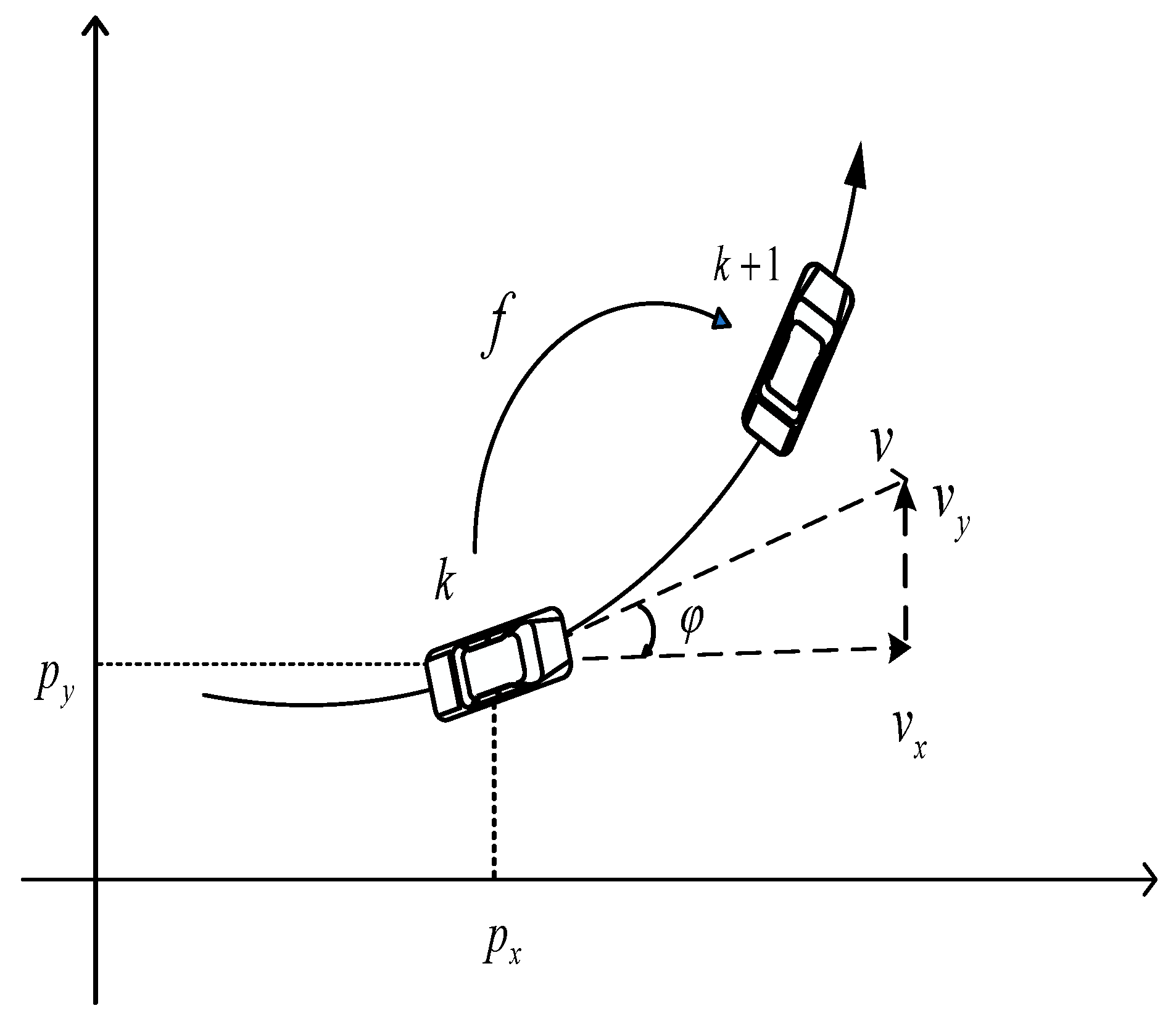
3.1. Constant Rotation and Acceleration Models

Figure 6 represents the kinematic model of the vehicle, in which the position coordinates of the vehicle include the vehicle speed, the vehicle swing angle, the current moment, the next moment, and the state transfer equation, which describes the change in the vehicle’s state of motion at consecutive points in time.

Specifically, the state information of the vehicle at the current moment is known, such as vehicle position, speed, acceleration, swing angular velocity, etc., and the state information of the vehicle at the next moment can be inferred through the state transfer equation, so that the cycle is iterative; each calculation is based on the results of the previous calculation, and the vehicle state information can be estimated at any time in the future.

The state variables $x={[p_x p_y v \theta a \omega ]}^T$ of the constant rate of rotation and acceleration model are chosen, where $a$ is the acceleration of the vehicle. The mathematical relationship between each state quantity is shown in the following equation.

$$\left[\begin{array}{c}{\dot{p}}_x\\ {\dot{p}}_y\\ \dot{v}\\ \begin{array}{c}\begin{array}{c}\dot{\theta }\\ \dot{a}\end{array}\\ \dot{\omega }\end{array}\end{array}\right]=\left[\begin{array}{c}v\cos (\theta )\\ v\sin (\theta )\\ a\\ \begin{array}{c}\begin{array}{c}\omega \\ 0\end{array}\\ 0\end{array}\end{array}\right]$$

(10)

Equation (10) is integrated over a sampling time $T=t_{k+1}-t_k$ to calculate the increment of each state quantity of the vehicle over a sampling time. The state transfer equations for the constant rate and acceleration model are easily obtained as shown in the following equation:

$$x_{k+1}=x_k+{\displaystyle {\int }_{t_k}^{t_{k+1}}\left[\begin{array}{l}{\dot{p}}_x\\ {\dot{p}}_y\\ \dot{v}\\ \dot{\theta }\\ \dot{a}\\ \dot{\omega }\end{array}\right]}dt$$

(11)

where $x_k$ denotes the state quantity of the vehicle at the current moment, and $x_{k+1}$ denotes the state quantity of the vehicle at the next moment. After the integral solving and simplification, the state transfer equations for the constant rate of rotation and acceleration model can be finally obtained.

When ${\omega }_k\ne 0$,

$$x_{k+1}=x_k+\left[\begin{array}{c}{\displaystyle \frac{a_k[\cos ({\omega }_{k}T+{\theta }_k)-\cos ({\theta }_k)]}{{\omega }_k^2}}+{\displaystyle \frac{(v_k+a_{k}T)\sin ({\omega }_{k}T+{\theta }_k)-v_k\sin ({\theta }_k)]}{{\omega }_k}}\\ {\displaystyle \frac{a_k[\sin ({\omega }_{k}T+{\theta }_k)-\sin ({\theta }_k)]}{{\omega }_k^2}}-{\displaystyle \frac{(v_k+a_{k}T)\cos ({\omega }_{k}T+{\theta }_k)-v_k\cos ({\theta }_k)]}{{\omega }_k}}\\ a_{k}T\\ {\omega }_{k}T\\ 0\\ 0\end{array}\right]$$

(12)

When ${\omega }_k=0$,

$$x_{k+1}=x_k+\left[\begin{array}{c}(v_{k}T+0.5a_k{T}^2)\cos ({\theta }_k)\\ (v_{k}T+0.5a_k{T}^2)\cos ({\theta }_k)\\ a_{k}T\\ {\omega }_{k}T\\ 0\\ 0\end{array}\right]$$

(13)

3.2. Traceless Kalman Filtering

The constant slew rate and acceleration model state transfer equations considering Gaussian white noise are shown below [16]:

$$x_{k+1}=f(x_k,{\psi }_k)$$

(14)

where $f$ is the state transfer equation adding the system noise, $\psi$ is the system noise, and the covariance matrix is the Gaussian noise $Q$.

The observation equation considering Gaussian white noise is as follows:

$$z_{k+1}=h(x_{k+1})+{\nu }_{k+1}$$

(15)

where $h$ is the measurement equation that maps the state space to the measurement space $v$ is the measurement noise, and the covariance matrix is the Gaussian noise $R$. The steps of the whole traceless transformation are as follows:

(1)

Generate Sigma points

In traceless Kalman filtering, a set of Sigma points is first generated from the mean and covariance matrices of the a priori states. In this case, the $n$ dimension needs to be selected as $2n+1$ Sigma sample points, and the selection formula for each Sigma sample point is as follows:

$$\{\begin{array}{l}{\chi }^{(0)}=\overline{x}\\ {\chi }^{(i)}=\overline{x}+{(\sqrt{(n+\lambda )P_x})}_i,i=1,2,\cdots n\\ {\chi }^{(i+n)}=\overline{x}+{(\sqrt{(n+\lambda )P_x})}_{i+n}\end{array}$$

(16)

where $\overline{x}$ is the mean value of the state variable and $P_x$ is the covariance matrix of the state variable $x$. $\lambda ={\alpha }^2\left(n+k\right)-n$ indicates how far away the Sigma sample points are from the mean value, and the further away, the smaller the weight, where $\alpha$ is the scale factor, which determines the degree of diffusion of the set of Sigma points. In general $0\le \alpha \le 1$, and $k$ is the scale factor, and there are no specific setup restrictions, but $(n+\lambda )p$ should be guaranteed to be a semipositive definite matrix at least.

The corresponding weights for each Sigma sample point are as follows:

$$W_m^{(i)}=\{\begin{array}{l}\lambda /(n+\lambda ),i=0\\ 1/2(n+\lambda ),i\ne 0\end{array}$$

(17)

where $\beta$ is the higher order characterization of the response state information, for a Gaussian distribution where $\beta =2$.

(2)

Obtain new Sigma sample points by nonlinear transformation

After generating the Sigma, these points are mapped to a nonlinear space by a nonlinear transformation. The Sigma sample points are mapped to the new space by a nonlinear equation of state [17]:

$$Y_{k+1|k}^i=f({\chi }^{(i)})$$

(18)

(3)

Calculate the weighted mean and covariance of the mapped Sigma sample points

An approximation of the nonlinear transformation can be obtained by a weighted average of the transformed Sigma sample points. The weighted mean and covariance of the mapped Sigma sample points are as follows:

$$\{\begin{array}{l}{\widehat{x}}_{k+1|k}={\displaystyle \sum _{i=0}^{2n}(W_m^{(i)})}{Y}_{k+1|k}^{(i)}\\ P_{k+1|k}={\displaystyle \sum _{i=0}^{2n}(W_c^{(i)})}(Y_{k+1|k}^{(i)}-{\widehat{x}}_{k+1|k}){(Y_{k+1|k}^{(i)}-{\widehat{x}}_{k+1|k})}^T+Q_k\end{array}$$

(19)

Similarly, the Sigma sample points are mapped to the new space by the nonlinear observation equation:

$${\zeta }_{k+1\mid k}^{(i)}=h({\chi }^{(i)})$$

(20)

Measurement means and covariances are calculated as follows:

$$\{\begin{array}{l}{\widehat{z}}_{k+1|k}={\displaystyle \sum _{i=0}^{2n}}(W_m^{(i)}){\zeta }_{k+1|k}^{(i)}\\ P_{zz,k+1|k}={\displaystyle \sum _{i=0}^{2n}}(W_c^{(i)})({\zeta }_{k+1|k}^{(i)}-{\widehat{z}}_{k+1|k}){({\zeta }_{k+1|k}^{(i)}-{\widehat{z}}_{k+1|k})}^T+R_k\\ P_{xz,k+1\mid k}={\displaystyle \sum _{i=0}^{2n}}(W_c^{(i)})({\zeta }_{k+1|k}^{(i)}-{\widehat{x}}_{k+1|k}){({\zeta }_{k+1|k}^{(i)}-{\widehat{x}}_{k+1|k})}^T\end{array}$$

(21)

To calculate Kalman gain and update state estimates and covariances, the following equations are used:

$$\{\begin{array}{l}{K}_{k+1}=P_{xz,k+1|k}{(P_{zz,k+1|k})}^{-1}\\ P_{k+1|k+1}=P_{k+1|k}-K_{k+1}{P}_{zz,k+1|k}{K}_{k+1}^T\\ {\widehat{x}}_{k+1|k+1}={\widehat{x}}_{k+1|k}+K_{k+1}(z_{k+1}-{\widehat{z}}_{k+1|k})\end{array}$$

(22)

As a result, the state estimate of the vehicle at the next moment is obtained based on the state information of the vehicle at the current moment, and the state information of the vehicle at any moment in the future can be obtained by simply iterating the state transfer equation continuously and repeating the above steps [18].

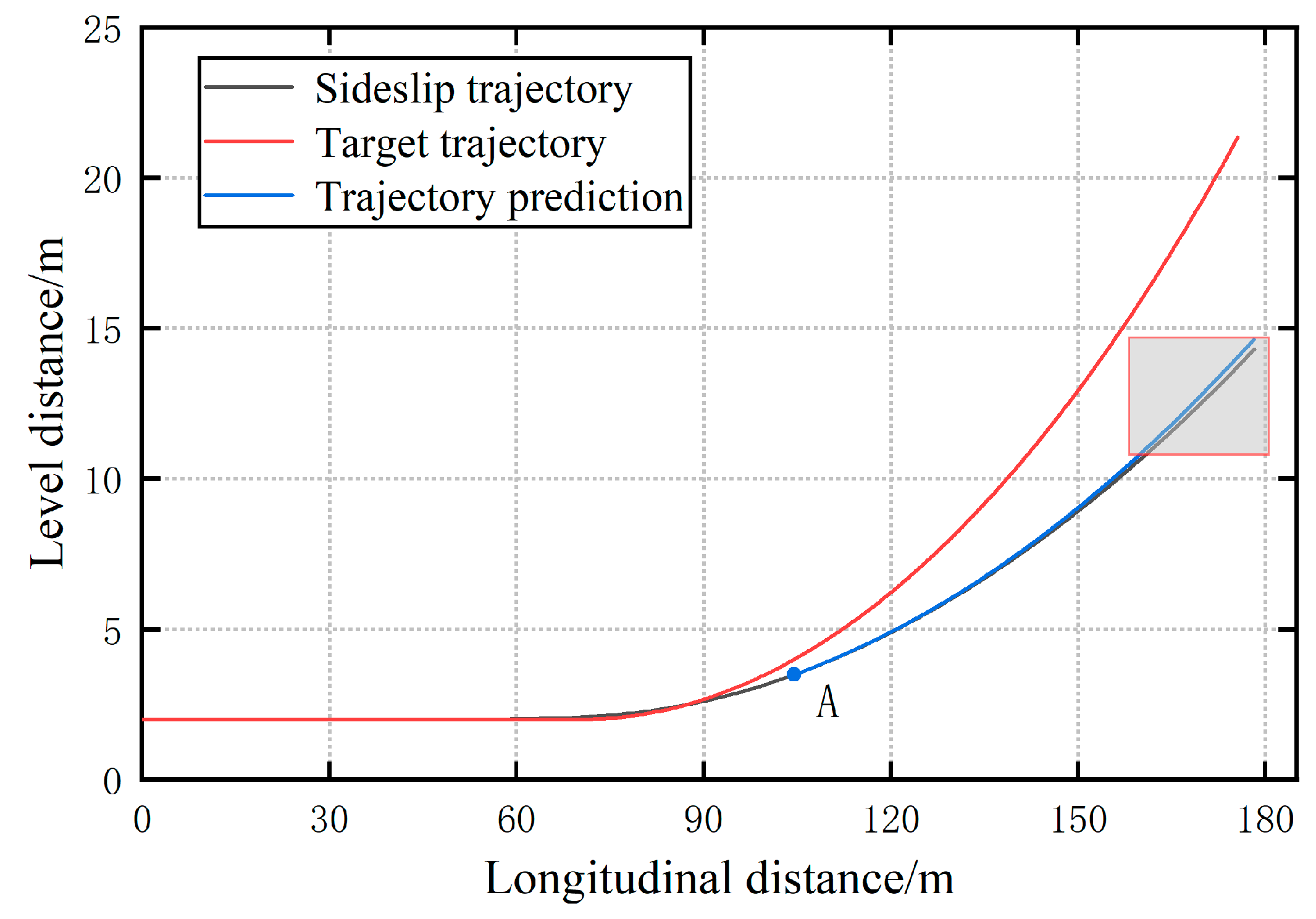
3.3. Potential Future Areas for Sideslip Vehicles

The uncertainty of vehicle trajectory prediction is processed by traceless Kalman filtering, and the prediction information of the vehicle state at any future moment is obtained [19]. These mainly include the horizontal and vertical coordinates of the future trajectory $x,y$ of the vehicle and its mean ${\mu }_1,{\mu }_2$, variance ${\sigma }_x,{\sigma }_y$, and covariance ${\rho }_{xy}$. Based on this information, the possible motion region of the vehicle after a sideslip is inferred under the condition of a given probability $P$. The corresponding joint probability distribution function is expressed as follows:

$$\begin{array}{l}f(x,y)={\displaystyle \frac{1}{2\pi {\sigma }_x{\sigma }_y}}{\displaystyle \frac{1}{\sqrt{1-{\rho }_{xy}^2}}}\\ \cdot \exp \left\{-{\displaystyle \frac{1}{2}}\left[{\displaystyle \frac{{\left(x-{\mu }_1\right)}^2}{{\sigma }_x^2}}-{\displaystyle \frac{2{\rho }_{xy}\left(x-{\mu }_1\right)\left(y-{\mu }_2\right)}{{\sigma }_x{\sigma }_y}}+{\displaystyle \frac{{\left(y-{\mu }_2\right)}^2}{{\sigma }_y^2}}\right]\right\}\end{array}$$

(23)

The possible elliptical region of the center of mass of a sideslip vehicle is obtained by derivation [20]:

$${\left[{\displaystyle \frac{1}{\sqrt{1-{\rho }_{xy}^2}}}\left({\displaystyle \frac{x-{\mu }_1}{{\sigma }_x}}\right)+{\displaystyle \frac{{\rho }_{xy}}{\sqrt{1-{\rho }_{xy}^2}}}\left({\displaystyle \frac{y-{\mu }_2}{{\sigma }_y}}\right)\right]}^2+{\left({\displaystyle \frac{y-{\mu }_2}{{\sigma }_y}}\right)}^2=t_p^2$$

(24)

In the formula, $t_p=\sqrt{-2\cdot \ln (1-p)}$.

We approximate the contour radius of the vehicle and the elliptical region in which the vehicle may appear by adding a vehicle radius to each of the long and short axes of the above ellipse.

4. Results

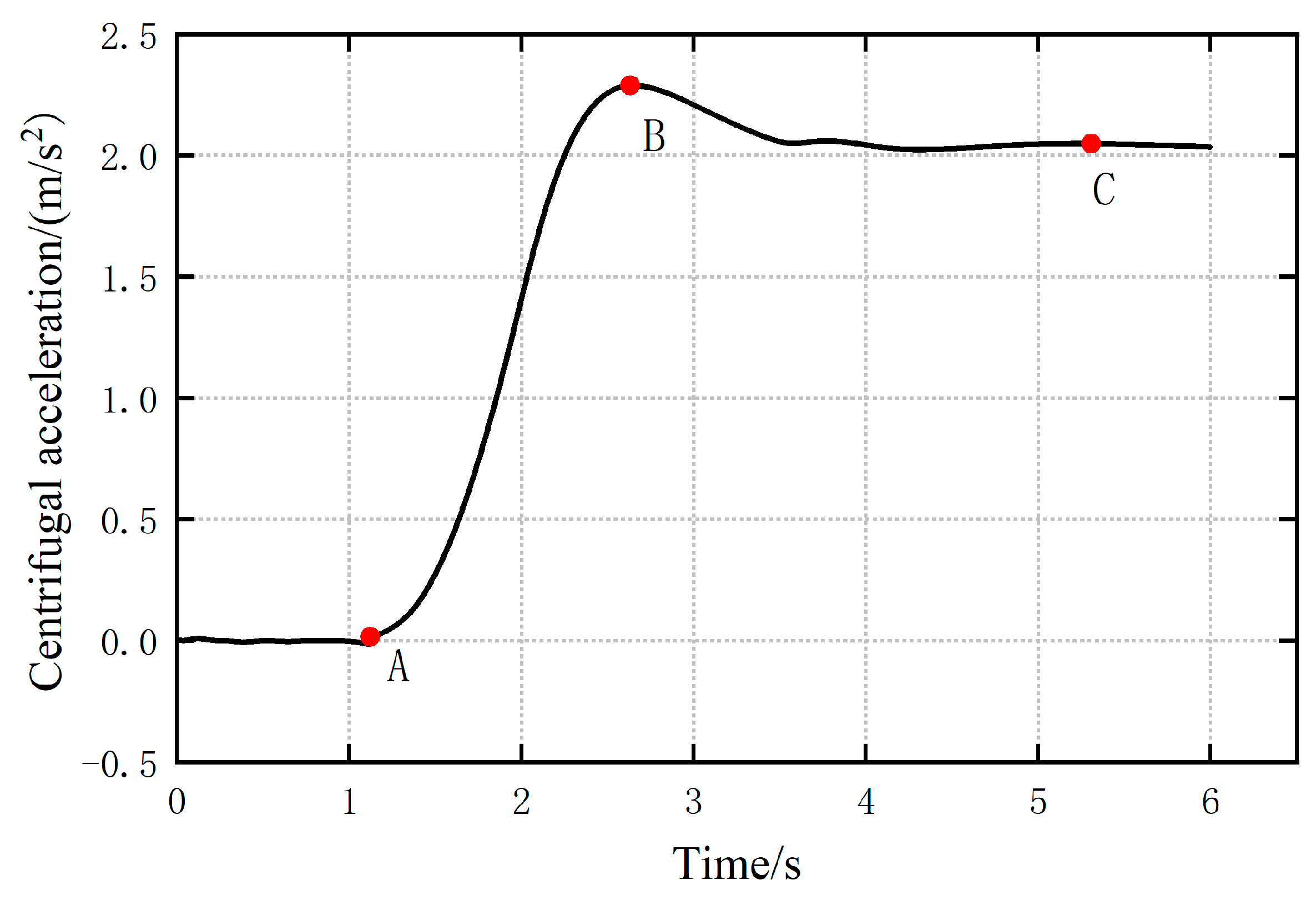
4.1. Pickup Truck Curve Sideslip Recognition

The working conditions were set as follows: initially, the pickup truck decelerated in the middle lane at 120 km/h, and after 70 m, it drove into a curve with a curvature of 1/300, in which the pavement adhesion coefficient of the whole road was 0.3, and the gradient was set at 0.01.

The centrifugal acceleration change curve of the pickup truck is shown in Figure 7. Before the pickup truck entered the curve and traveled along the curve, its centrifugal acceleration was approximately 0, and the pickup truck did not skid. Then, the pickup truck entered the curve and traveled along the curve, and its centrifugal acceleration increased continuously and reached the maximum value at 2.55 s. Then, the centrifugal acceleration began to decrease. The sideslip recognition module in the process of recognition will be in front of the pickup truck at point B, with centrifugal acceleration judgment for the extreme value.

The distance between the edge of the front pickup truck and the lane line, the lateral speed relative to the lane line, and the time at which the edge arrives at the lane line are analyzed, and it is determined whether or not they simultaneously reach the thresholds set. Therein, the threshold value of the distance between the edge of the front vehicle and the lane line is set to 0.5 m; the threshold value of the lateral speed of the front vehicle with respect to the lane line is set to 0.2; and the threshold value of the time for the edge of the front vehicle to arrive at the lane line is set to 1 s. As can be seen from Figure 8, Figure 9 and Figure 10, the lateral speed of the forward pickup truck relative to the lane line exceeded the thresholds set therein at 2.55 s; then the time for its edge to arrive at the lane line and the distance from the lane line are drastically shortened, and the pickup truck rapidly approaches the lane line on one side and ultimately reaches the respective thresholds set therein at 2.74 s and 3.12 s, respectively. As a result, at 3.12 s, all three sideslip characterization indicators reached their respective set thresholds, and the pickup truck can be determined to be a potentially dangerous sideslip vehicle.

4.2. Sideslip Recognition of SUV Vehicle on Curve

The working conditions are set as follows: at first, the SUV slowed down in the middle lane at a speed of 110 km/h, then entered a bend with a curvature of 1/300 after 70 m, and then a second dangerous sideslip occurred to change lanes. The road adhesion coefficient of the whole road is 0.3, and the slope is set to 0.03.

The centrifugal acceleration curve of the SUV is shown in Figure 11, which shows that the centrifugal acceleration of the SUV is approximately zero at the beginning of the straight-line driving, and no sideslip occurs. After the SUV enters a curve, its centrifugal acceleration increases continuously and reaches the maximum value in 2 s, and then the centrifugal acceleration begins to decrease gradually.

Unlike the pickup truck, which experienced the first type of sideways slide, the SUV vehicle did not slide out of its lane at this point, although it was moving closer to the left lane line and further away from the right lane line. As can be seen in Figure 12, Figure 13 and Figure 14 first, the lateral velocity of the SUV vehicle in front relative to the lane line reaches its set threshold at 3.69 s, and then its edge arrival time to the right lane line and distance from the right lane line reach their respective thresholds set at 4.72 s and 5.32 s, respectively. Therefore, the SUV vehicle was finally determined as a potentially hazardous sideswipe vehicle at 5.32 s.

4.3. Pickup Truck Normal Sideslip Recognition

The working conditions were set as follows: initially, the pickup truck decelerated in the middle lane at 110 km/h, and after 70 m, it drove into a curve with a curvature of 1/500, followed by a normal sideslip. In this case, the road surface adhesion coefficient for the whole road was 0.5 and the gradient was set to 0.01.

As can be seen in Figure 15, Figure 16 and Figure 17, the sideways speed of the pickup truck in front relative to the lane line reached its set threshold at 2.70 s, and then the time it took for its edge to reach the right lane line and the distance from the right lane line gradually decreased, but neither reached their respective set thresholds. Therefore, although the pickup truck had some sideslip at this point, it would not be recognized as a dangerous sideslip.

4.4. Pickup Truck Curve Sideslip Trajectory Prediction

The working conditions were set as follows: the pickup truck decelerated in the middle lane at 120 km/h, and after 70 m, it drove into a curve with a curvature of 1/300, and was recognized as a dangerous sideslipping vehicle by the autopilot vehicle at 3.12 s. Here, the road surface adhesion coefficient for the whole road was 0.3, and the gradient was set to 0.01.

The constant rate of rotation and acceleration model was used to predict the sideslip trajectory of the pickup truck, as shown in Figure 18. The pickup truck first followed the target trajectory, but sideslipping occurred after entering the curve. The sideslip recognition model recognizes that a dangerous sideslip has occurred in the vehicle in front at point A. The trajectory prediction model starts to predict the sideslip trajectory of the vehicle in front, as shown by the blue curve in Figure 18.

In the first half of the trajectory prediction, the sideslip trajectory and the predicted trajectory basically coincide, and the prediction error is small, as shown in Figure 19 and Figure 20. However, because the parameters of the constant rotation rate and acceleration model are fixed and there is no way to adjust them, and because the state of the vehicle in front of the vehicle is changing at any time, which results in the offset between the predicted trajectory and the sideslip trajectory with the growth of prediction time, the prediction error gradually increases.

4.5. Areas Where Sideslip May Occur for Vehicles

Figure 21 represents the propagation of uncertainty in the prediction of the sideslip trajectory of a pickup truck with a probability of 0.9. The black dashed line in the figure represents the predicted sideslip vehicle trajectory, and the blue ellipse represents the area of the future contour that may occur after the vehicle has sideslipped. At the initial stage of sideslip trajectory prediction, the accuracy of prediction is relatively high, the error is small, and the area of the ellipse region is small; however, with the passage of time, the error gradually accumulates, the accuracy of trajectory prediction decreases, and the area of the ellipse region is gradually enlarged, which indicates that the uncertainty in the predicted trajectory is also increasing. However, because the speed of the sideslip vehicle is fast and the time to slide out of the lane it is in is also shorter, the prediction of the sideslip trajectory of the front vehicle will not take too long.

5. Discussion

(1) Using the different sideslip scenarios to categorize the front vehicle sideslip into dangerous sideslip and ordinary sideslip, four sideslip feature indicators quantitatively describing their characteristics were extracted, and a front vehicle sideslip recognition strategy was constructed, which was combined with the sideslip feature indicators to determine whether the vehicle in front of it was experiencing sideslip or not.

(2) A constant rate of rotation and acceleration model was constructed to use the state information of the front skidding vehicle at that moment in the constant rate of rotation and acceleration model to predict the future trajectory of the front skidding vehicle. Then, the uncertainty in the trajectory prediction process was handled by using the traceless Kalman filter, and the possible future vehicle contour region of the front skidding vehicle was derived under the condition of a probability of 0.9.

The simulation results show that the trajectory of the front skidding vehicle can be effectively predicted in a short time using the constant rate of rotation and acceleration model, with high accuracy and small errors. In the future, further research should be conducted to combine the emergency collision avoidance strategy of self-driving vehicles under destabilizing conditions such as a tire blowout of the vehicle in front.

References

- Huang, H.; Yang, M.; Wang, C.; Wang, B. Collision warning system based on front vehicle behavior recognition. J. Huazhong Univ. Sci. Technol. (Nat. Sci. Ed.) 2015, 43 (Suppl. S1), 117–121. [Google Scholar]
- Monot, N.; Moreau, X.; Benine-Neto, A.; Rizzo, A.; Aioun, F. Comparison of rule-based and machine learning methods for lane change detection. In Proceedings of the 2018 21st International Conference on Intelligent Transportation Systems (ITSC), Maui, HI, USA, 4–7 November 2018; pp. 198–203. [Google Scholar]
- Xiong, S. Analysis of Expressway Merging Behavior and Optimization of Merging Area Organization. Master’s Thesis, Jilin University, Changchun, China, 2019. [Google Scholar]
- Cai, Y.; Tai, K.; Wang, H.; Li, Y.; Chen, L. Research on vehicle behavior recognition algorithm around driverless cars. Automot. Eng. 2020, 42, 1464–1472. [Google Scholar]
- Zhu, L.; Liu, L.; Zhao, X.; Yang, D. Research on vehicle driving behavior recognition based on support vector machine. Transp. Syst. Eng. Inf. 2017, 17, 91–97. [Google Scholar]
- Chung, S.; Lee, H. Vehicle sideslip estimation and compensation for banked road. Int. J. Automot. Technol. 2016, 17, 63–69. [Google Scholar] [CrossRef]
- Ma, B.; Liu, Y.; Gao, Y.; Yang, Y.; Ji, X.; Bo, Y. Estimation of vehicle sideslip angle based on steering torque. Int. J. Adv. Manuf. Technol. 2023, 94, 3229–3237. [Google Scholar] [CrossRef]
- Lai, E.-M.; Luo, Y.-T. Automobile center of mass side estimation based on multi-information fusion. Sci. Technol. Eng. 2024, 13, 1889–1894. [Google Scholar]
- Shirazi, M.S.; Morris, B.T. Looking at intersections: A survey of intersection monitoring, behavior and safety analysis of recent studies. IEEE Trans. Intell. Transp. Syst. 2021, 18, 4–24. [Google Scholar] [CrossRef]
- Mozaffari, S.; Al-Jarrah, O.Y.; Dianati, M.; Jennings, P.; Mouzakitis, A. Deep learning-based vehicle behavior prediction for autonomous driving applications: A review. IEEE Trans. Intell. Transp. Syst. 2020, 23, 33–47. [Google Scholar] [CrossRef]
- Zhang, R.; Cao, L.; Bao, S.; Tan, J. A method for connected vehicle trajectory prediction and collision warning algorithm based on V2V communication. Int. J. Crashworthiness 2017, 22, 15–25. [Google Scholar] [CrossRef]
- Lefkopoulos, V.; Menner, M.; Domahidi, A.; Zeilinger, M.N. Interaction-aware prediction for autonomous driving: A multiple model kalman filtering scheme. IEEE Robot. Autom. Lett. 2020, 6, 80–87. [Google Scholar] [CrossRef]
- Okamoto, K.; Berntorp, K.; Di Cairano, S. Driverintention-based vehicle threat assessment using random forests and particle filtering. IFAC-PapersOnLine 2017, 50, 13860–13865. [Google Scholar] [CrossRef]
- Wang, Y.; Liu, Z.; Zuo, Z.; Li, Z.; Wang, L.; Luo, X. Trajectory planning and safety assessment of autonomous vehicles based on motion prediction and model predictive control. IEEE Trans. Veh. Technol. 2019, 68, 8546–8556. [Google Scholar] [CrossRef]
- Xiang, Y.; He, Y.; Luo, Y.; Bu, D.; Kong, W.; Chen, J. Recognition model of sideslip of surrounding vehicles based on perception information of driverless vehicle. IEEE Intell. Syst. 2022, 37, 79–91. [Google Scholar] [CrossRef]
- Wang, P.-C. Research on Dynamic Vehicle Trajectory Prediction Method in Lanes. Master’s Thesis, Chang’an University, Xi’an China, 2021. [Google Scholar]
- Xiang, Y. Highway Forward Vehicle Instability Identification and Emergency Collision Avoidance Decision Planning Method. Ph.D. Thesis, Chongqing University, Chongqing, China, 2023. [Google Scholar]
- Wang, Y.; Wang, C.; Zhao, W.; Xu, C. Decision-Making and planning method for autonomous vehicles based on motivation and risk assessment. IEEE Trans. Veh. Technol. 2021, 70, 107–120. [Google Scholar] [CrossRef]
- Qu, W. Research on Driving Behavior Recognition and Trajectory Prediction Method for Traffic Vehicles. Master’s Thesis, Jilin University, Changchun, China, 2021. [Google Scholar]
- Althoff, M.; Mergel, A. Comparison of Markov chain abstraction and Monte Carlo simulation for the safety assessment of autonomous cars. IEEE Trans. Intell. Transp. Syst. 2020, 12, 1237–1247. [Google Scholar] [CrossRef]
Disclaimer/Publisher’s Note: The statements, opinions and data contained in all publications are solely those of the individual author(s) and contributor(s) and not of MDPI and/or the editor(s). MDPI and/or the editor(s) disclaim responsibility for any injury to people or property resulting from any ideas, methods, instructions or products referred to in the content. |
© 2025 by the authors. Published by MDPI on behalf of the World Electric Vehicle Association. Licensee MDPI, Basel, Switzerland. This article is an open access article distributed under the terms and conditions of the Creative Commons Attribution (CC BY) license (https://creativecommons.org/licenses/by/4.0/).
Share and Cite
Ou, J.; Cheng, X.; Zhang, P. Research on Trajectory Prediction Based on Front Vehicle Sideslip Recognition. World Electr. Veh. J. 2025, 16, 241. https://doi.org/10.3390/wevj16040241
Ou J, Cheng X, Zhang P. Research on Trajectory Prediction Based on Front Vehicle Sideslip Recognition. World Electric Vehicle Journal. 2025; 16(4):241. https://doi.org/10.3390/wevj16040241
Chicago/Turabian StyleOu, Jian, Xiaolong Cheng, and Pengju Zhang. 2025. "Research on Trajectory Prediction Based on Front Vehicle Sideslip Recognition" World Electric Vehicle Journal 16, no. 4: 241. https://doi.org/10.3390/wevj16040241
APA StyleOu, J., Cheng, X., & Zhang, P. (2025). Research on Trajectory Prediction Based on Front Vehicle Sideslip Recognition. World Electric Vehicle Journal, 16(4), 241. https://doi.org/10.3390/wevj16040241