Re-Evaluation of the Impacts of Dietary Preferences on Macroinvertebrate Trophic Sources: An Analysis of Seaweed Bed Habitats Using the Integration of Stable Isotope and Observational Data

Abstract

Stable isotope analyses of food webs have been used in previous decades to determine trophic sources and food web structures. The use of stable isotope models to estimate consumption contributions is based on a type of multivariate beta distribution called the Dirichlet distribution. The Dirichlet distribution does not conclude the p_i = 0 and p_i = 1 situation. Thus, scientists have previously assumed that every potential trophic source contributes to consumption in stable isotope models. However, animals have dietary preferences and some trophic resources may not contribute to consumption. Less is known about the effects of species-specific dietary processes on stable isotope analyses, especially in regard to trophic contribution estimation. In this study, we develop methods to determine consumers’ “real potential trophic sources” and “discrimination factors” using lab-based observations and lab-based discrimination experiments. We describe a dietary process-based stable isotope mixing model (D-SIMM) that integrates lab-based dietary preference observations and the stable isotope mixing model (SIMM) to estimate trophic contributions. Then, we present the application of D-SIMM on three representative macroinvertebrate species in our study area (sea urchin: Anthocidaris crassispina (A. crassispina); gastropod: Turbo cornutus (T. cornutus); and mussel: Septifer virgatus (S. virgatus)) to re-evaluate source-consumer contributions. Thus, we compare the differences between the source contribution estimation results of SIMM and D-SIMM by calculating the standardized convex hull area (TA) of species-specific trophic sources and the consumer standard ellipses area (SEA) of the potential trophic source group. Three examples illustrate significant differences in species-specific dietary preferences between consumers, resulting in systematic difference for TA, SEA and trophic source contribution estimation results between SIMM and D-SIMM. As such, D-SIMM explains p_i = 0 of certain trophic sources, which often causes uncertainty and is ignored in previous SIMM research. In addition, species-specific discrimination factors should be noticed during trophic source estimation. For estimation of the trophic contribution of source-consumers, our findings imply that the dietary preferences of consumers should be fully considered before SIMM analysis, and that D-SIMM is a more ecological process and robust measure. Additionally, we found high macroalgae (MAC) coverage in seaweed beds and a high detritus contribution of MAC to sedimentary organic matter (SOM). These findings, combined with the high contributions of MAC and SOM to consumers, suggest that MAC and its debris are the basal trophic sources for gastropods, sea urchins and mussels in seaweed bed habitats. The conservation of seaweed beds should be fully considered to ensure sustainable utilization of shellfish.

1. Introduction

Understanding the structure and function of habitats requires information on trophic interactions, energy and material flow patterns [1,2,3]. The seaweed bed is acknowledged as the most productive habitat on earth, and its net primary production (NPP) can reach as high as 0.5–3.5 kg·C/m² per year [4,5]. In seaweed bed habitats, benthic primary producers (e.g., macroalgae and microphytobenthos) and pelagic primary producers (e.g., phytoplankton) provide abundant food sources for grazing food chains [6]. Thus, large amounts of detritus produced by primary producers are transported by hydrodynamic forces and the sedimentation-resuspension effect, leading to a complex composition of sedimentary organic matter (SOM) and suspended particulate organic matter (SPOM). This provides more attractive trophic sources for the detritus food chain [7,8]. In general, macroalgae, microphytobenthos, phytoplankton and their detritus (both SOM and SPOM) make up trophic source diversity and there is a strong benthos–pelagic coupling effect in seaweed bed habitats [9,10].

The high trophic source diversity in seaweed bed habitats can influence secondary production assemblage through either the grazing food chain or the detritus food chain, especially in macroinvertebrate communities [11]. In marine ecosystems, secondary production is the linkage between primary producers and higher trophic level organisms through the utilization of food sources, the support of all species, from the prey to the top consumer (bottom-up), and the increased complexity of the food web structure [12,13]. In the past, studies on functional groups have helped determine the relationship between diversity, community structure, and function, and to get a clear idea about the material and energy flow in ecosystems. Descriptions of secondary production assemblages in seaweed beds have revealed a high level of diversity and species abundance. However, the material and energy flow across functional groups of primary and secondary production have been less studied than natural patterns, abundance or biomass [14].

In view of the trophic complexity and the lack of description of material and energy flow patterns in seaweed bed habitats, it is clear that alternative and quantitative procedures are needed to estimate the relationship between trophic sources and different functional groups of consumers. Numerous techniques have been used to draw inferences, which can be grouped into two types of procedures: indirect approaches, such as stable isotope analysis, protein analysis and fatty acid analysis; and direct approaches, such as gut content analysis (including gut content digest proportion and content frequency) and dietary observations (including descriptions of motivation, consumption and dietary preferences) [15,16,17]. In particular, the stable isotopes analysis (SIA) and stable isotope mixing model (SIMM) are commonly used to analyze food-web structures. Trophic interactions and analysis of animal diet compositions are done by calculation of the relative contribution of each food source to the diet [18]. In recent studies, the rapid growth of SIMM methods has integrated the SIMM with Bayesian frameworks, the Markov Chain Monte Carlo (MCMC) sampling procedure, measurement errors, and source and mixture process errors to provides a fully consistent statistical foundation. However, although SIMM tools (such as IsoSource, IsoError, MixSIR, SIAR, IsotopeR, and MixSIAR) have improved our ability to utilize solid statistical foundations to partition ecological process features (for example, the different contributions of dietary sources, different assimilation efficiencies for dietary sources, and variation associated with predicted discrimination factors), they still have several limitations [19]. In general, the SIMM framework is based on a multivariate beta distribution, known as the Dirichlet distribution, which excludes the p_i = 0 situation. Specifically, in SIMM, every trophic source in the food-web is treated as a “potential source” and assumed to contribute to consumers. Further, each consumer is considered to be a generalist species. However, this may cause bias during the estimation of source contribution to specific consumers (Figure 1).

Ogle suggested the most critical limitation of SIMMs is that they provide limited mechanistic insight [20]. Specifically, they do not explicitly incorporate additional models or data reflecting underlying processes that affect the source contribution estimation. The above limitations of the assumptions of SIMMs (Figure 1) lead to underlying and fundamental problems of stable isotope analyses. What are the real potential food sources of macroinvertebrates and how will dietary selection affect the prediction of SIA? Fortunately, direct approaches can overcome the above limitations and illustrate species-specific interactions between trophic sources and consumers. Nevertheless, due to the small-size spectrum of many trophic sources (such as phytoplankton, POM) and macroinvertebrates, or feeding behaviors (such as grazing or filter-feeding) of some consumers, it is extremely difficult to obtain sufficient and reliable data for stomach analysis to allow prey identification. In this case, lab-based observation is a more appropriate method for qualitative evaluation of species-specific selection strategies and the supply of information about p_i = 0 and p_i = 1 situations [21,22].

Our study has three main objectives: (1) to determine the macroinvertebrate dietary types in seaweed beds by dietary observation and identify their real dietary sources; (2) to estimate the contribution of dietary sources to macroinvertebrates in seaweed beds by SIMMs; and (3) to verify the results of dietary observations and the SIMMs dietary contribution estimation by investigation of the δ¹³C and δ¹⁵N stable isotope signatures of trophic sources and consumers to solve the uncertainty and discrepancies between the traditional stable isotope technique and consumer–diet interactions; and (4) to investigate the use of a new framework named D-SIMM that combines dietary observation data and stable isotope analysis data, to recalculate the trophic resource contributions of different potential trophic sources.

2. Materials and Methods

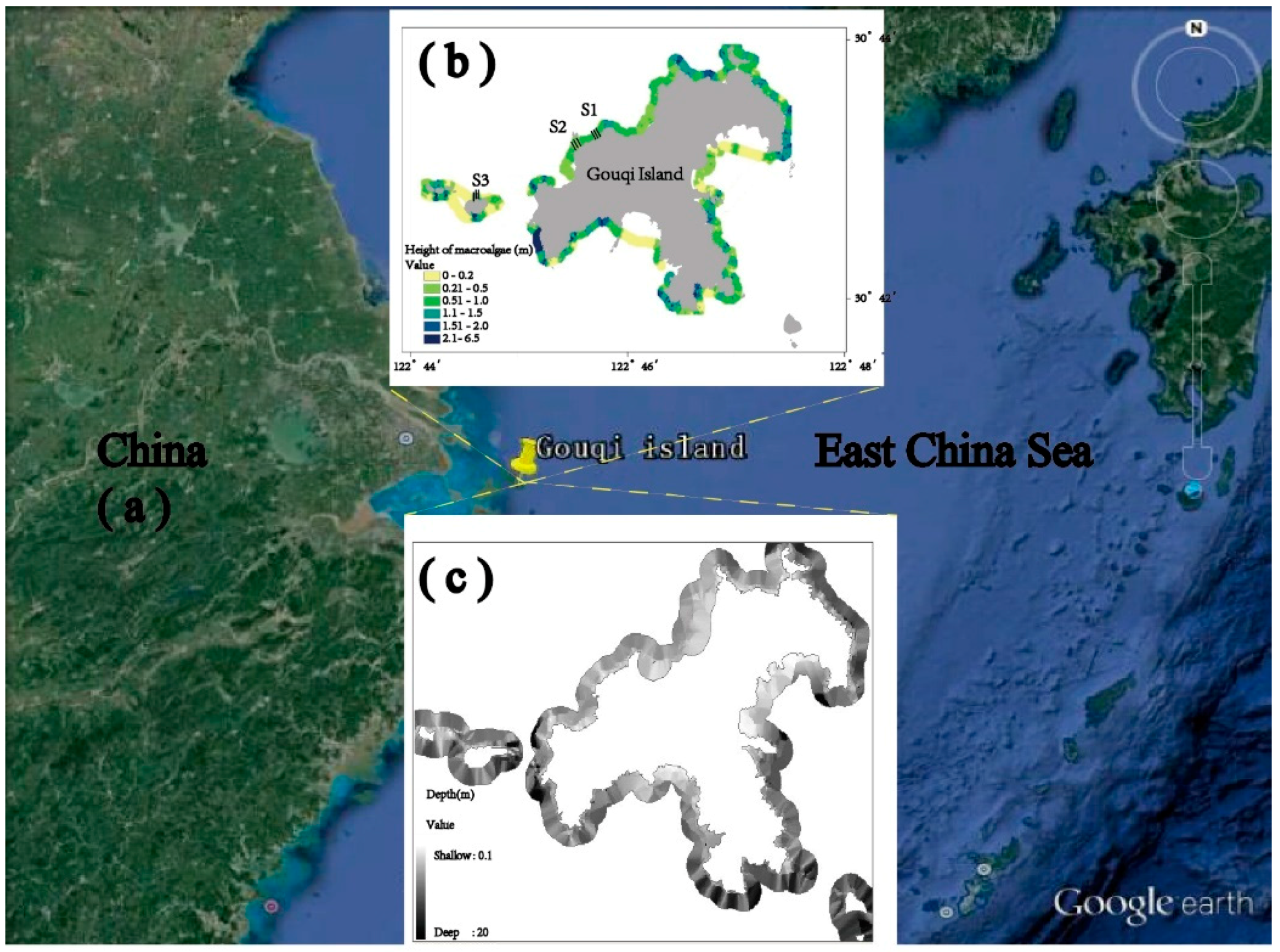
2.1. Study Site

The Gouqi Island seaweed bed (GISB) is located in the Maan Archipelago Marine Protect Area (MAMPA) of the East China Sea (Figure 2). The environment within the MAMPA is a consequence of low traditional fishery activities, minimal fishery activity disturbance and strict management control. Field studies were conducted in subtidal areas, which are largely flat and consist of fine sediment and cobble beds with a relatively subtidal rocky slope, extending about 30 m along and 15 m perpendicular to the shore. A high coverage of diverse macroalgae (MAC) and abundant phytoplankton (PHY) were recorded in GISB in a previous study [23]. Despite the above potential source of grazing food chain, SOM (e.g., sediment mix with a range of benthic microalgae, visible as a thick brown-green film on the rock), SPOM and particulate organic matter in bottom layer (BPOM) comprise the detritus food chain source in the GISB habitat. Various food sources of both grazing and detritus food chains and rocky reef slopes make up the seaweed bed habitat. In this study, MAC, SOM, SPOM and BPOM were assumed to be potential food sources in the study area.

2.2. Sampling

2.2.1. Potential Food Sources

The water depth, temperature, salinity and dissolved oxygen in water were measured monthly at the sample site. In addition, we used a Biosonic-DX sonar detector to estimate the coverage and height of MAC. The average macroalgae coverage was more than 80% of the study site; all environmental results mentioned above are presented elsewhere. Samples were collected from the study site (Figure 2), seasonal from May 2013 to May 2015. Three sampling stations (400 m × 50 m) and nine line transects (50 m) were randomly set across the depth gradients of line transects in seaweed bed habitats (S1, S2 and S3).

Four groups of potential food sources were sampled: macroalgae (MAC), sedimentary organic matter (SOM), suspended particulate organic matter (SPOM), and benthic particulate organic matter (BPOM). Underwater sampling was conducted by scuba diving over a period of 2–3 consecutive days (seasonal). Quadrat frame samplers (30 cm × 30 cm) were used to sample the MAC. MAC were qualified from three replicate quadrat frame samplers set across the depth gradients of line transects (1 m each, 1–5 m, n = 15/transect) in seaweed bed habitats (S1, S2 and S3). Using a fine mesh dipnet (25-μm mesh), MAC within the samplers were collected, rinsed in distilled water to remove associated organisms and then immediately frozen in plastic bags on the boat. The MAC samples were run in two separate analyses. In the first analysis, 13 species of fresh MAC were fed as the diet during the diet selection observation. In the second analysis, 13 species of MAC were stored in individual bags and preserved in a cooled state for posterior stable isotope analyses. Thus, the MAC were classified into dominant species of macroalgae (DMAC, IRI > 20 or Y > 0.02) and rare species (IRI < 20 or Y < 0.02) according to the IRI and Y of the macroalgae community used in a previous study.

IRI = (N + W) F × 10⁴,

where N stands for the abundance of species i as a proportion of the total abundance, W stands for the proportion of species i in the total biomass, and F stands for the species occupancy frequency.

$$Y=\frac{n_i{f}_i}{N}$$

where n_i stands for the number of individuals, N stands for the total number of MAC, and f_i stands for the frequency of MAC i.

For each site, samples of sediment organic matter (mixed vegetative sediment, detritus and phytomicrobenthos) were obtained (seasonal) with a designed sediment trap (2 cm width × 20 cm height) dug on the rocky surface from May 2013 to May 2014. Three replicate sediment traps were set across the depth gradient line transects (1 m each, 1–5 m, n = 15/transect). Every other week, we took the sediment and interstitial water samples by scuba diving with the trap tube, placed them in 2 L PVC bottles and froze them. We classified the sedimentary organic matter in the seaweed bed habitats as SOMA and that outside the seaweed bed as SOMB.

Phytoplankton samples were obtained from seaweed habitats with a phytoplankton net (mesh size = 35 μm). The samples were washed with distilled water, filtered through two experimental bolt panels (250 μm mesh, 160 μm mesh) and a GF/F membrane (0.7 μm pore size, Waterman: Ningbo, China). To remove the organic matter on the membrane, the membrane had been heated in a muffle furnace at 550 °C for 6 h before the experiment. Membrane samples were examined under a light microscope to confirm that they were free of zooplankton; all filter phytoplankton samples were then frozen.

A water sampler was used to collect three 2 L samples from both the surface and bottom layers of water. These were maintained on ice and transported to the laboratory within 4 h. SPOM and BPOM samples were filtered through an experimental bolt panel (250 μm mesh) and GF/F membrane (0.45 μm pore size, Waterman, Ningbo, China). As with the phytoplankton samples, the SPOM and BPOM membrane samples were examined under a light microscope to confirm that they were free of zooplankton, and then, they were frozen.

2.2.2. Consumers

Three representative macroinvertebrate samples (gastropod, sea urchin and mussel) were collected from the study site (see Section 1) by scuba diving from May 2013 to May 2015 (seasonal) from the three sampling stations, as previously described.

The macroinvertebrate samples were run in two separate analyses: a stable isotope analysis and lab-based diet observations. For the stable isotope analysis, 17 sea urchins (A. crassispina), 26 gastropods (T. cornutus) and 41 mussels (S. virgatus) were run in the stable isotope analysis. Muscle tissue from gastropods (foot tissue) and mussels (adductor) and gonads from sea urchins were excised, rinsed in distilled water and frozen in plastic bags.

2.3. Species-Specific Diet Selection Observation

Lab-based diet observations were completed in 60 L macroinvertebrate feeding tanks (Figure 3) for six weeks (July–August 2013) in the Gouqi Island laboratory; 576 gastropods and 576 sea urchins were obtained from three sites (S1, S2, and S3) by scuba diving. In the laboratory, we simulated the average field environmental conditions (e.g., 20 °C constant mean temperature, with 0.7–1.4 μmol/L and 0.13–0.30 μmol/L total phosphorous, and 4.91 ± 1.74 mg/L dissolved organic carbon). Gastropods and sea urchins obtained from the field were immediately sent to the laboratory and put in macroinvertebrate feeding tanks. Both species were then left to equilibrate to tank conditions and were starved for two days prior to the diet selection experiments. The lab-based experiments were run in two separate trials: species-specific dietary selection and species-specific discrimination.

The dietary selection experiments of gastropod and sea urchin all involved single diet treatments (16 tanks each time, replicated six times). A single diet treatment consisted of feeding an adequate amount of a single potential food source (from 13 species of MAC, POM, PHY and SOMA, see details in

Table 1. Stable isotope ratio (δ¹³C and δ¹⁵N, n = sample size, mean, SD) of potential diet sources and consumers in the GISB habitat during the two-years/urvey (May 2013 until May 2015).

Sample	Sample Size (n)	δ13C (‰)		δ15N (‰)
		Mean	SD	Mean	SD
Potential trophic source
PHY	12	−20.64	0.92	5.84	2.02
SPOM	10	−20.92	0.86	6.69	0.62
BPOM	11	−15.42	1.63	8.76	1.88
SOMA	12	−18.38	0.73	2.75	0.24
SOMB	18	−21.95	0.51	2.53	0.51
MADS	39	−14.55	3.08	4.99	1.55
Corallina officinalis	3	−8.48	0.73	6.6	0.55
Jania decussato-dichotoma	3	−8.93	0.74	6.82	0.36
Ulva pertuca	11	−14.3	0.41	5.76	1.26
Dictyopteris dichotoma	3	−14.77	3.19	5.06	1.26
Sargassum vachellianum	5	−15.72	2.81	4.53	1.03
Sargassum horueri	10	−16.83	1.54	3.8	1.59
Sargassum fusiforme	4	−16.7	0.7	3.84	0.54
MARS	22	−17.04	1.6	5.29	1.2
Garteloupia livida	3	−14.45	0.51	4.55	0.09
Chondria crassicaulis	3	−16.83	1.28	5.31	2.94
Undaria pinnatifida	7	−16.39	0.65	5.17	0.84
Codium fragile	3	−18.54	0.29	5.26	1.08
Ceramium japonicum	3	−19.16	0.25	6.23	0.22
Hypnea cervicornis	3	−18.55	0.34	5.78	0.61
Consumers
Gastropod (T. cornutus)	26	−16.3	0.85	5.86	0.54
Sea urchin (A. crassispina)	17	−15.44	0.65	5.08	0.5
Mussel (S. virgatus)	41	−15.97	0.64	6.15	0.62

PHY, phytoplankton; SPOM, suspended particulate organic matter; BPOM, benthic particulate organic matter; SOMA, sedimentary organic matter in the seaweed bed; SOMB, sedimentary organic matter outside the seaweed bed; MADS, dominant species of macroalgae; MARS, rare species of macroalgae.

) to six consumers (gastropod or sea urchin) in each tank. All potential macroinvertebrate food sources were collected from the same habitat (sampling procedure shown in Section 2.2). These food sources were chosen since they are different functional primary producer groups and represent the potential trophic source diversity in a seaweed bed habitat. Each day, food and filtered seawater were changed, MAC and SOMA were weighed, concentrations of PHY and SOMA were detected, and dead consumers were removed to minimize bias during the diet process of consumers (e.g., consumption of faces, decomposing MAC or PHY materials). The rates of MAC consumption and gastropod mortality were used to evaluate the dietary selection of macroinvertebrates. Specifically, if the mortality (M) of consumer M was >90%, we defined that the source as being unavailable for that consumer and removed the correspond stable isotope value from the source data pool. If 90% ≥ M ≥ 10%, we defined the source as a neutral source and retained the corresponding stable isotope value in the source data pool. If M < 10%, we defined the source as a favorable source for the consumer that corresponded to a stable isotope value in the source data pool.

Thus, the feeding functional group definition approach expands earlier methods by classifying predators based on mobility, feeding mode and diet preference mode with the following traits: mobility (mobile, semi-mobile, and sessile); feeding mode (jawed, tentaculate, and others, e.g., filter); and feeding preference (herbivore, carnivore, detritus feeders, and deposit feeders) [24,25].

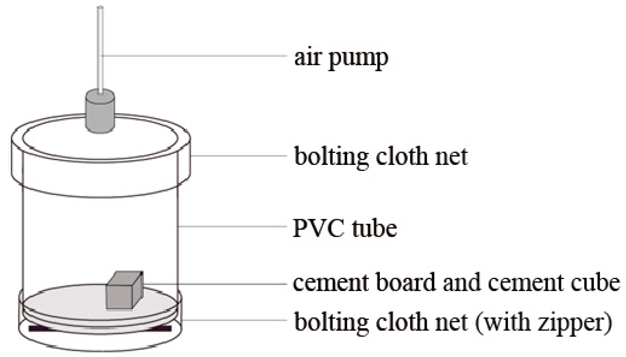
2.4. Estimation of Discrimination between Diets and Macroinvertebrates

The species-specific selection experiments indicated that some sources could be eliminated while previous research reported that some sources could be combined. Beyond the diet selection, discrimination factors, defined as isotopic shifts between the diet and consumer, were assumed to be valid for all trophic levels in a previous study. However, the present study showed that the discrimination factor values are consumer-diet specific [26]. To monitor the discrimination factor values of macroinvertebrates and to allow precise estimation of the potential range of potential contribution, we used the second D-SIMM trial (e.g., discrimination factor) to design species-specific discrimination (or fractionation) values (Δ). After 42 days of diet observation, gastropod foot muscle tissue and sea urchin gonads were removed for the stable isotope analysis.

2.5. Stable Isotope Analysis

In the laboratory, all stable isotope analysis samples (consumers: gastropod foot tissue, mussel adductors and sea urchin muscle; prey: MAC, SOM, SPOM, BPOM, and PHY; see details in Table 1) were cleaned with deionized water and then dried at −60 °C and lyophilized for 36 h until weight stabilized.

The stable isotope ratios (¹³C/¹²C and ¹⁵N/¹⁴N) of samples were analyzed by mass spectrometry (Isotope Ratio Mass Spectrometer Flash EA 1112, HT-Delta V Advantages, Thermo Fisher Scientific, Waltham, MA, USA) at Shanghai Ocean University.

$$\mathsf{\delta }\mathrm{X}(‰)=\left[\left({\mathrm{R}}_{\mathrm{sample}}/{\mathrm{R}}_{\mathrm{standard}}\right)\right]\times {10}^3$$

where X represents ¹³C or ¹⁵N and R is the ¹³C/¹²C or ¹⁵N/¹⁴N ratio. Pee Dee Belemnite standard (PDB) and atmospheric N₂ were used as the carbon and standard, respectively [27].

We described the diet-consumer specific discrimination (Δ) with the following formula:

$$\overline{{\Delta }^{13}C}=\frac{{{\displaystyle \sum }}_{i=1}^n\left({\delta }^{13}{C}_{consumer,i}-{\delta }^{13}{C}_{diet,i}\right)}{n},$$

$$\overline{{\Delta }^{15}N}=\frac{{{\displaystyle \sum }}_{i=1}^n\left({\delta }^{15}{N}_{consumer,i}-{\delta }^{15}{N}_{diet,i}\right)}{n}.$$

where $\overline{{\Delta }^{13}C}$ is the average δ¹³C discrimination of consumer (%) to diet i, ${\delta }^{13}{C}_{consumer,i}$ is the δ¹³C value of consumer after 42 days of feeding with diet i, n is the total number of diet items consumed, $\overline{{\Delta }^{15}N}$ is the average δ¹⁵N discrimination of the consumer (%) to diet i, and ${\delta }^{15}{N}_{consumer,i}$ is the ${\delta }^{15}N$ value of the consumer after 42 days of feeding with diet i.

The standard deviations (SD) of ${\Delta }^{13}C$ were calculated as

$$S{D}_{{\Delta }^{13}C}=\sqrt{\frac{1}{n}{\displaystyle \sum }_{i=1}^n{\left({\delta }^{13}{C}_{consumer,i}-{\delta }^{13}{C}_{diet,i}\right)}^2}.$$

The standard deviations (SD) of ${\Delta }^{15}N$ were calculated as

$$S{D}_{{\Delta }^{15}N}=\sqrt{\frac{1}{n}{\displaystyle \sum }_{i=1}^n{\left({\delta }^{15}{N}_{consumer,i}-{\delta }^{15}{N}_{diet,i}\right)}^2}.$$

To estimate the contributions of certain diets more precisely, the carbon and nitrogen values of consumers were corrected prior to inclusion in MixSIAR using species-specific $\overline{{\Delta }^{13}C}$, $\overline{{\Delta }^{15}N}$, $S{D}_{{\Delta }^{13}C}$ and $S{D}_{{\Delta }^{15}N}$, and the details are shown in Table 4.

2.6. Data Analysis

Statistical analyses were performed in R, version 3.2.4 [28]. To estimate the approximate potential trophic source contributions to representative macroinvertebrate species, three species-specific models (gastropod, sea urchin and mussel) were constructed based on integration of the mixing model, MixSIAR, and dietary preference observation data. MixSIAR (V. 3.1.6 program, Brian Stock et al.) is a Bayesian mixing model that improves simpler linear mixing models; it incorporates several years of advances in the Bayesian mixing model theory by explicitly including the uncertainty in source values, categorical and continuous covariates and prior information [29]. In MixSIAR, estimations of the contribution of posterior probability sources to macroinvertebrates were simulated by Markov chain Monte Carlo sampling (e.g., MCMC sampling, chain length = 1,000,000, burn in = 50,000, thin = 500, chains = 3) and the following isotopic information was incorporated into the model: Firstly, means and standard deviations of sources based on previous SIMM hypotheses (all consumers have the same diet) and the diet selection experiment (consumers have species-specific diet selection and some trophic resources may have no contribution to certain consumers) were included. Source data were selected based on the criteria described in the diet observation section. Secondly, the mean values and standard deviations of species-specific diet-consumer discrimination were included. In this study, we assumed that ${\Delta }^{13}{C}_{sea urchin}=1.93\pm 1.1$ and ${\Delta }^{13}{C}_{gastropod}=0.43\pm 0.13$, based on a lab-based experiment. In addition, ${\Delta }^{13}{C}_{mussel-PHY}=2.17\pm 0.32$, ${\Delta }^{13}{C}_{mussel-MAC}=0.35\pm 0.35$, ${\Delta }^{13}{C}_{mussel-SOM}=0.99\pm 0.74$, and ${\Delta }^{13}{C}_{mussel-POM}$ were calculated for mussels in lab-based discrimination experiments in a previous study (see details in Table 4). As for ${\Delta }^{15}N$, we assumed the general values of ${\Delta }^{15}{N}_{gastropod}=1.43\pm 0.8$ and ${\Delta }^{15}{N}_{sea urchin}=0.80\pm 0.20,$ based on the diet selection experiment. In addition, ${\Delta }^{15}{N}_{mussel-MAC}=3.45\pm 0.21$, ${\Delta }^{15}{N}_{mussel-SOM}=3.37\pm 0.59$, ${\Delta }^{15}{N}_{mussel-POM}=3.33\pm 0.71$, and ${\Delta }^{15}{N}_{mussel-PHY}=3.78\pm 0.29$ because in the mussel consumer-diet, ${\Delta }^{15}N$, which was summarized in a previous reference (Table 4). Thirdly, consumer isotopic signature data (raw data of single consumer) were used. Fourth, a Dirichlet distribution was used prior to the proportion estimation (recommended by Jackson et al. and incorporated in Moore et al. [30,31]).

The differences between of mean isotopic signatures (SOMA vs. SOMB and BPOM vs. SPOM) and discrimination values were tested using Student’s t tests and Fisher’s F tests [32]. Then, before the isotopic width analysis, we used two default diagnostic tests to test the MCMC posterior estimation: Gelman–Rubin and Geweke tests [33]. To compare the trophic niche estimation results between SIMM and D-SIMM, multivariate ellipse metrics were tested under a hypothesis-testing framework proposed by Jackson et al. [30]. This analysis generates standard ellipse areas (SEA) which are bivariate equivalents to standard deviations in a univariate analysis. We used SEA values corrected for small sample size (SEA_C) to calculate the niche overlap and generate Bayesian estimates of SEA (SEA_B) to test differences in trophic niches by comparing their 95% credible limits. Thus, a comparison of trophic contribution estimation between SIMM and D-SIMM was established based on hypotheses from previous studies (all consumers have the same diet) and this study (inputting species-specific diet selection information, respective data pool based on our diet selection and source-consumer specific discrimination).

Furthermore, as Saitos mentioned, estimations of source–macroinvertebrate interactions have often been static approximations [34]. Therefore, due to the lack of species-specific stable isotope turnover time information, we used muscles and gonads to represent a long period to allow a stable isotope analysis of diet, and we assumed the observed stable isotope values were representative of average source–macroinvertebrate interactions over the year model.

3. Results

3.1. Dietary Observations: Mobility, Mode and Preference

Dietary observation experiments of three representative macroinvertebrates were conducted to illustrate the functional group categories of each species and to obtain a precise description of the diet-macroinvertebrate interaction relationship. Following the dietary observation experiment, three representative macroinvertebrates were classified into two functional groups: sea urchins and gastropods are semi-mobile jawed surface omnivores and mussels are sessile filter-feeders (

Table 2. Potential trophic sources and diet–macroinvertebrate trophic interactions.

Description	Species	Functional Group	Potential Trophic Source
			MAC	PHY	SOM	POM
Sea urchin	A. crassispina	Semi-mobile jawed surface omnivore (herbivore and detritus feeder)	●a	×c	○b	○b
Gastropod	T. cornutus	Semi-mobile jawed surface omnivore (herbivore and detritus feeder)	●a	×c	●a	○b
Mussel	S. virgatus	Sessile filter-feeder (MAC and PHY and POM and SOM)	●a	●a	●a	●a

M: mortality; ●^a: M < 10%; ○^b: 90% ≥ M ≥ 10%; ×^c: M > 90%.

). Although sea urchins and gastropods belong to the same functional group, the MAC-specific selection experiments showed differences in selection strategy between sea urchins and gastropods (

Table 3. Prey selection of gastropods and sea urchins during MAC-species-specific selection experiments.

Potential Trophic Source	Replicate Number of Experiments (n)	Macroinvertebrate—MAC Dietary Preference
		Sea Urchin	Gastropod
Chlorophyta
Ulva pertuca	6	●a	●a
Codium fragile	6	○b	×c
Rhodophyta
Ceramium japonicum	6	○b	○b
Chondria crassicaulis	6	○b	×c
Corallina officinalis	6	×c	×c
Jania decussato dichotoma	6	×c	×c
Hypnea cervicornis J.Ag.	6	○b	×c
Garteloupia kurogii	6	●a	●a
Phaeophyta
Sargassum fusiforme	6	●a	●a
Sargassum horueri	6	●a	●a
Dictyopteris dichotoma	6	●a	○b
Ishige okamurai	6	●a	○b
Hizikia fusifarme	6	●a	●a

M: mortality; ●^a: M < 10%; ○^b: 90% ≥ M ≥ 10%; ×^c: M > 90%.

): sea urchins showed a more generalist diet selection for MAC. Specifically, Codium fragile, Chondria crassicaulis and Hypnea cervicornis J.Ag. could be only utilized by sea urchins, and sea urchins showed a higher survival rate when fed Sargassum horueri and Ishige okamurai. Moreover, calcareous red algae (Corallina officinalis and Jania decussato-dichotoma) could not be consumed by sea urchins or gastropods. Mussels were able to feed on MAC, PHY, SOM and POM; in this case, we used all potential stable isotope information for the estimation of the diet composition of mussels [23].

3.2. Stable Isotope Analysis and Source Contribution Evaluation

There was a large difference in both the macroinvertebrate species-specific data pool and macroinvertebrate-MAC-specific selection data pool (

Table 4. Δ¹³C and Δ¹⁵N (trophic enrichment factors or discrimination) values in various macroinvertebrates.

Group	Tissue	Diet	Lab. or Field	Δ13C (‰)	Δ15N (‰)	SDΔ13C (‰)	SDΔ15N (‰)	Ref.
Bivalves (M. veneriformis)	Muscle	POM	Lab.	0.9	3.6			[35]
Bivalves (R. philippinarum)	Muscle	POM	Lab.	0.6	3.4			[35]
Bivalves (C. sandai)	Soft tissue	PHY	Lab.	0.7	2.1			[36]
Bivalves (M. edulis)	Muscle	PHY	Lab.	2.17	3.78	0.324	0.292	[37]
Bivalves (C. gigas)	Muscle	PHY	Lab.	1.85	3.79	0.194	0.194	[37]
Bivalves (C. sandai)	Soft tissue	MAC	Lab.	0.6	3.6			[36]
Bivalves (C. sandai)	Soft tissue	MAC	Lab.	0.1	3.3			[36]
Bivalves (Scallops)	Soft tissue	POM	Field	3.8	0.9			[38]
Bivalves (Mussel)	Soft tissue	POM	Field	3.4	1.8			[38]
Sea urchin (H. erythrogramma)	Muscle	MAC (Phaeophytes)	Lab.	1.85	2.44			[39]
Sea urchin (H. erythrogramma)	Muscle	MAC (Fleshy Rhodophytes)	Lab.	3.23	3.96			[39]
Sea urchin (H. erythrogramma)	Muscle	MAC (Calcareous Rhodophytes)	Lab.	4.39	3.02			[39]
Sea urchin (H. erythrogramma)	Muscle	MAC (Chlorophytes)	Lab.	1.2	3.15			[39]
Gastropod (T. torquatus)	Foot tissue	MAC (Fleshy Rhodophytes)	Lab.	−0.17	1.56			[39]
Gastropod (T. torquatus)	Foot tissue	MAC (Calcareous Rhodophytes)	Lab.	0.14	1.06			[39]
Gastropod (T. cornutus)	Foot tissue	MAC and SOM	Lab.	0.43	1.43	0.13	0.8	Present study
Sea urchin (A. crassispina)	Gonad	MAC and SOM	Lab.	1.93	0.8	1.1	0.2	Present study

MAC, macroalgae; PHY, phytoplankton; POM, particulate organic matter; SOM, sedimentary organic matter.

). The macroinvertebrate species-specific (Figure 4 and Figure 5) and source functional group (Figure 4,

Table 5. SIBER Standard Ellipses Area (95% credible interval) of each potential source group in SIMM, sea urchin D-SIMM and gastropod D-SIMM.

Source	TA	SEA	SEAC
	SIMM (gastropod and sea urchin)
DMAC	51.41	13.66	14.03
RMAC	16.79	6.09	6.39
SOMA	1.21	0.54	0.6
BPOM	20.35	9.48	10.54
SPOM	2.21	1.37	1.54
PHY	10.36	5.12	5.64
	Gastropod D-SIMM
DMAC	35.82	9.13	9.43
RMAC	10.9	4.98	5.44
SOMA	1.12	0.54	0.6
BPOM	20.35	9.48	10.54
	Sea Urchin D-SIMM
DMAC	35.82	9.13	9.43
RMAC	16.79	6.34	6.71
SOMA	1.12	0.54	0.6
BPOM	20.35	9.48	10.54

TA, total area; SEA, standard ellipses area; SEA_C, standard ellipse areas corrected for small sample size; SIMM, stable isotope mixture model; D-SIMM, dietary process-based stable isotope mixture model.

) SIBER results showed differences in the isotopic niche width between SIMM and D-SIMM. For the data pool sources (Figure 4 and Figure 5), significantly higher TA and δ¹³C values of SIMM implied that negligence of species-specific diet selection will significantly overestimate the trophic niche space and trophic source diversity. In addition, differences in CD, NND and SDNND between SIMM and D-SIMM (gastropod and sea urchin) should be noted since they indicate discrepancy in the average degree of source diversity of macroinvertebrates, prey redundancy and even the distribution of the source niche.

Similarly, for the macroinvertebrate-MAC-specific selection data pool, we adjusted the macroinvertebrate-MAC-specific selection effects in both DMAC and RMAC data pools. The SEA and SEA_C of DMAC and RMAC were different between SIMM and D-SIMM. The SEA and SEA_C indexes of D-SIMM were higher than those of the gastropod D-SIMM and sea urchin SIMM analyses (Table 5). The above comparison indicates that macroinvertebrate-MAC selection strategy is species-specific and affects the discrepancy of the structure of the source data pool.

After integrating the results from the dietary selection observation and the stable isotope discrimination data into MixSIAR, the species-specific sources contribution estimation and comparisons between SIMM and D-SIMM were established. Figure 6 represents the estimated proportions of each dietary source to the gastropods (Figure 6A), sea urchins (Figure 6B) and mussels (Figure 6C). The estimation of macroinvertebrate contribution varied notably with the inclusion of every potential source (SIMM, p_i≠ 0 situation) and the exclusion of certain potential sources (D-SIMM, p_i = 0 situation). Both SIMM and D-SIMM outcomes showed high variability in the relative contributions of the macroalgae-dominant sources (SOMA, DMAC and RMAC). It is noteworthy that, after excluding the p_i = 0 situation of both PHY and SPOM, the gastropods and sea urchins had broader confidence intervals of MAC (RMAC + DMAC, D-SIMM: 15.1% + 23.6% vs. SIMM: 22.0% + 14.7%), SOMA (D-SIMM: 50.5% vs. SIMM: 45.1%) and BPOM (D-SIMM: 10.9% vs. SIMM: 6.3%) in D-SIMM than in SIMM. Overall, SOMA was the most important resource in both species (gastropod: mean = 35.6% ± 9.9%, 95% interval: 14.4–54.8%; sea urchin: mean = 50.5% ± 9.7%, 95% interval: 30.9–68.1%). RMAC and DMAC also contributed as major dietary sources to both gastropods and sea urchins, whereas RMAC was the second most important dietary source for gastropods (28.0$\pm$18.2%, 95% interval: 1.3–65.4%) and sea urchins (23.6$\pm$15.1%, 95% interval: 1.4–55.4%) and DMAC was the third most important dietary source for gastropods (26.6$\pm$16.0%, 95% interval: 1.6–60.5%) and sea urchins (15.1 $\pm$ 10.1%, 95% interval: 0.9–41.1%). However, for mussels, BPOM was the main dietary source (mean = 44.3% $\pm$ 12.2%, 95% interval: 23.3–70.2%), followed by SOMA (mean = 24.3% $\pm$ 15.9%, 95% interval: 11.3–57.6%) (Figure 6C).

Moreover, although the 95% Bayesian interval range of each diet (SOMA, DMAC, RMAC and BPOM) in gastropod D-SIMM and sea urchin D-SIMM seemed to have a wider range of variation, the DIC value of gastropod D-SIMM (DIC = 600.36) was smaller than that of gastropod SIMM (DIC = 889.84) and the same trend was found for the comparison between sea urchin D-SIMM (DIC = 600.801) and sea urchin SIMM (DIC = 840.75) (Figure 6A,B). The DIC result showed that the D-SIMM result was more precise when diet proportion estimations were simulated by MCMC sampling (chain length = 1,000,000, burn in = 50,000, thin = 500, chains = 3).

4. Discussion

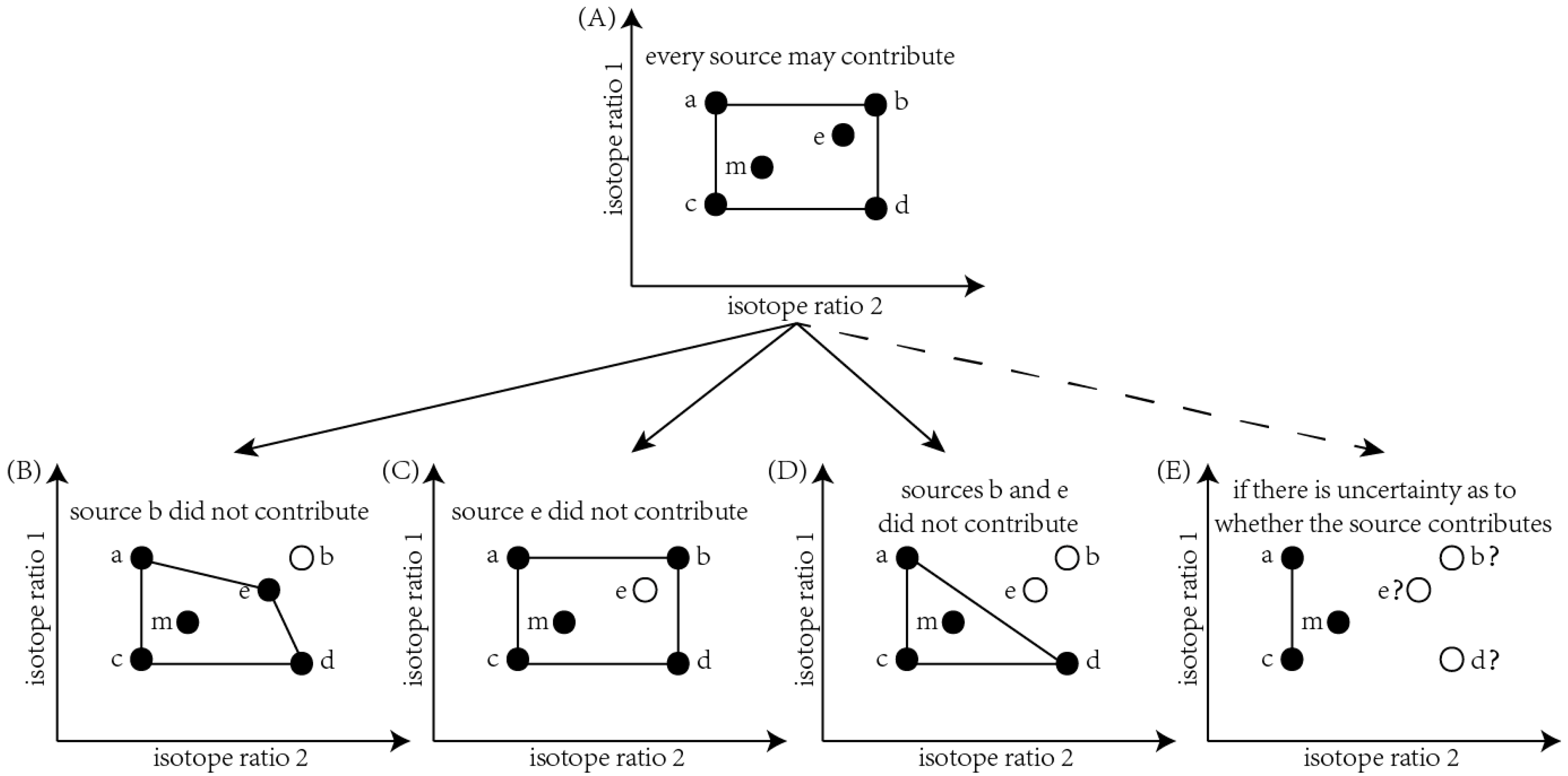
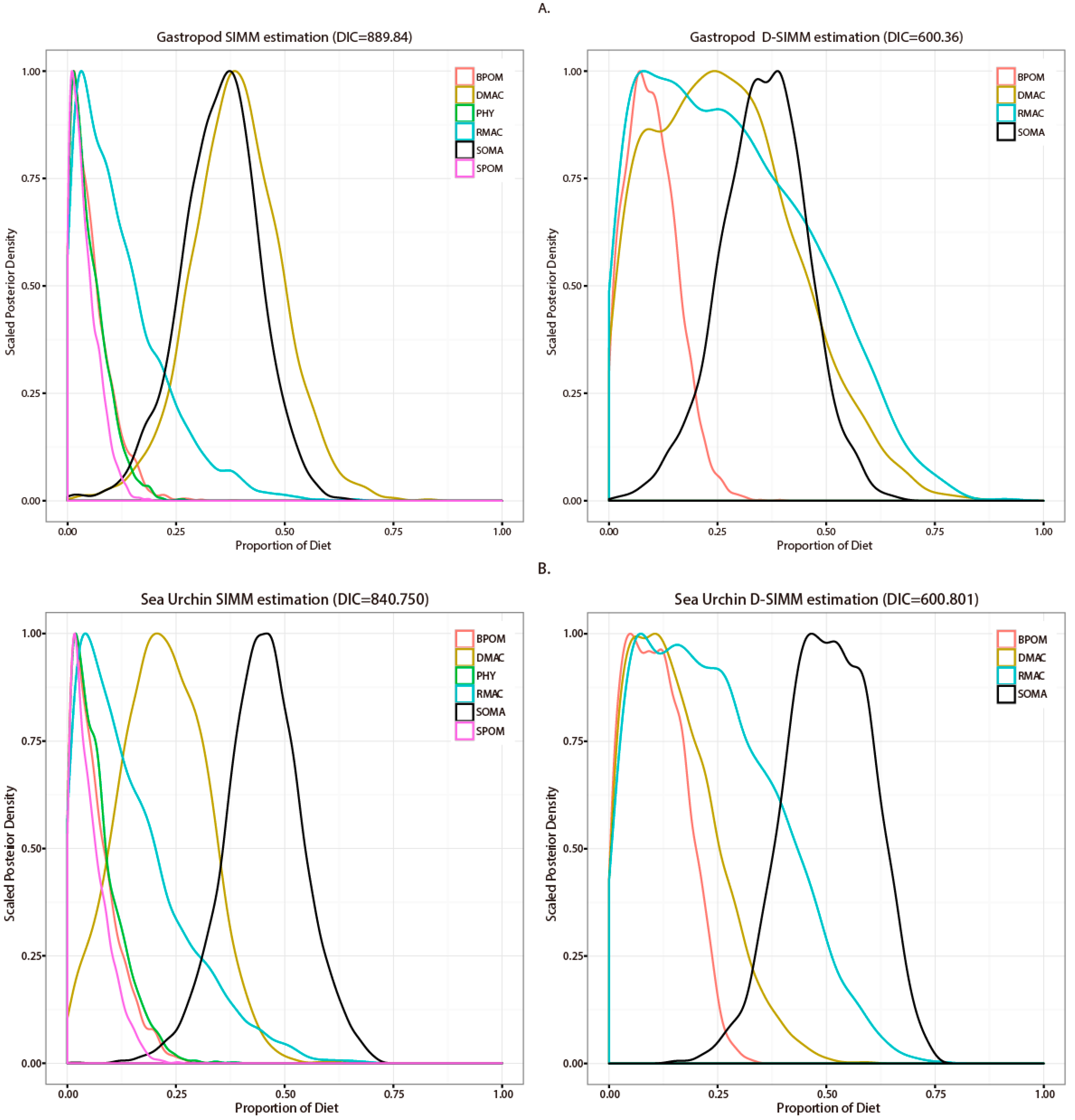
4.1. Comparison between SIMM and D-SIMM

The identification of important feeding links between sources and consumers, and the definition of trophic structure through stable isotope analysis has been an active area in the last 40 years. However, it was previously unknown whether a clear view of dietary preference effects on diet estimation could be achieved from SIMM. Further, what we could learn from understanding the complexity and intricate linkages between dietary preferences and the SIMM framework was also unknown. Information about animal diets leads to insight into trophic interactions and niche variability. Through diet observation experiments, we confirmed that gastropods (T. cornutus) and sea urchins (A. crassispina) are semi-mobile jawed surface omnivores. In addition, sea urchins showed a more generalist diet selection in terms of MAC. Several studies have shown methods to estimate source-specific discrimination factors based on the isotopic signatures of food sources. Our species-specific discrimination results indicated that the discrimination factors of macroinvertebrates are species-source-specific and are affected by a discrimination process in organism tissues. Species-source-specific discrimination factors should be determined by lab-based experiments before added into SIMM. These results agree with the macroinvertebrate–source relationship of a dietary selection strategy and species-specific discrimination values described by Gates for rocky reefs in Australia (gastropods and sea urchins) and for Lake Erie in USA (mussels) [39,40].

For comparison between source data pools, since ANOVA is based on Z-distribution and our mixture model is based on posterior framework (multivariate normal distribution), we did not use ANOVA to test the differences of posterior estimation contribution between D-SIMM and SIMM data pools. SIBER (Stable Isotope Bayesian Ellipses in R) is often used to compare isotopic niche widths among and within communities. Beyond describing individual components of a community and isotopic structure of functional groups, here, we used SIBER as a robust and objective tool to compare the structures of the SIMM and D-SIMM data pools and to illustrate how dietary preferences affect the estimation of sources. The SIBER results supported the proposal that dietary preferences have effects on the isotopic data pool: significant differences in the δ¹³C range, TA, CD, NND and SDNND were observed (Figure 4 and Figure 5) between SIMM and D-SIMM data pools (gastropods and sea urchins). For example, for the source data pool of SIMM, the TA was much higher than that in D-SIMM (Figure 5); for NND and SDNND, the value shifted after being added into the diet selection information. These results were mainly due to the inclusion (0 < p_i < 1, SIMM) or exclusion (p_i = 0, D-SIMM) of certain potential sources as possible contributions to representative macroinvertebrates, causing the uncertainty to increase when estimating the mixture (consumers) using source data in SIMM (Figure 1) [41]. The above fact shows how the dietary preferences of macroinvertebrates affect structure of the isotopic data pool. Meanwhile, significant differences in the TA, SEA and SEA_C of RMAC between gastropod and sea urchin D-SIMM (Table 5) were observed. For this reason, it is now clear that species-specific diet preferences of macroinvertebrates will alter the isotopic data pool structure and cause bias during the mixing process in SIMM and MCMC simulations.

Beyond using standard ellipses and Bayesian methodology to demonstrate how dietary preference affects isotopic data pools, SIMM and D-SIMM provide a distinct framework to investigate ecological effects on diet contribution estimation by addressing issues related to ecological factors in stable isotope mixture models. In the SIMM framework, changes to the mean diet contribution have been related to changes in dietary source concentrations, assimilation efficiencies and discrimination factors. Accordingly, in a D-SIMM framework, experimental studies extend the cause of variation in diet contribution estimation to the dietary preference of consumers and variance of species-source-specific discrimination processes. In this case, a large difference in diet contribution estimation was shown between SIMM and D-SIMM (Figure 6). In comparison, between SIMM and D-SIMM, significant differences in diet proportion and high variability in terms of 95% Bayesian interval were observed in both gastropod and sea urchin D-SIMM (for example, gastropod–DMAC SIMM: 17.9–60.0% vs. gastropod–DMAC D-SIMM: 1.6–60.5%; gastropod–RMAC SIMM: 0.4–37.7% vs. gastropod–RMAC D-SIMM: 1.3–65.4%).

As diet estimates were used as inputs for other models, formally selecting the best estimate could allow for more accurate input to other models [42,43,44]. A likelihood-based estimation of parameters allows for formal model selection, using criteria such as Akaike’s information criteria (AIC), Bayesian information criteria (BIC) and deviance information criteria (DIC), so that distinct alternative hypotheses can be evaluated in a statistically rigorous way [45,46]. In our study, we used deviance information criteria (DIC) for model selection. The DIC is a hierarchical modelling generalization of the AIC and BIC, where the posterior distributions of the models have been obtained by MCMC simulation [47]. In contrast to existing SIMM models, the D-SIMM can incorporate various dietary processes via the process model and has relatively lower DIC values. Our results showed that D-SIMM (Figure 6) is a more appropriate and precise model for tackling diet proportion estimation issues.

4.2. Diet Estimation of Representative Macroinvertebrate Species in Seaweed Beds

Food-webs in typical habitats have become a hot topic and have attracted attention worldwide, especially in highly productive and diverse habitats such as seaweed beds. However, due to the trophic source diversity in the seaweed bed habitat, the small-size spectrum of both primary and secondary production, and the feeding habits (such as grazing or filter-feeding) of certain predators, it is extremely difficult to supply sufficient and reliable data for a quantitative source–consumer relationship analysis of prey identification [48]. Meanwhile, although the components of potential sources in seaweed beds in GISB were isotopically distinct making the identification of the macroinvertebrate–source relationship feasible, the development of strong inferences required experimental manipulation of macroinvertebrate-specific diet selection strategies when multiple sources existed in the habitat. For indirect approaches, such as the SIA used in our study, the most critical limitation is SIA; it cannot provide taxa-specific information and it sometimes has difficulty confirming the ingestion of materials in the food-web. This was illustrated by the SIMM results whereby, without species-specific diet selection information the PHY and SPOM were shown to make contributions to both gastropods (T. cornutus) and sea urchins (A. crassispina) (Figure 6), while the diet selection experiment showed they cannot (p_i = 0) feed on PHY and SPOM (Table 2). Thus, although both gastropods (T. cornutus) and sea urchins (A. crassispina) were shown to use MAC as a food source (Table 2), difference diet selection preferences for MAC were still found in species-specific MAC selection experiments (Table 3). Our D-SIMM showed that D-SIMM could be used for the quantitative estimation of species–diet interactions in those which could not do stomach analyses.

The seaweed bed represents a subtidal complex system of pools characterized by a rich macroinvertebrate abundance and diversity, as well as a rich macroalgae community [49]. It is clear that there is a large difference in diet proportion estimations between different macroinvertebrate functional groups. Briefly, the multivariate analysis revealed two main pathways in seaweed beds: the detritus food chain and the grazing food chain. The detritus food chain had detritus (BPOM, SPOM and SOMA) as the main basal sources and mussel is a representative species of the detritus food chain. Specifically, BPOM and SOMA were observed as the main diets of mussels in seaweed bed habitats (Figure 6C). The second pathway is based on a grazing food chain and is composed of species that rely on macroalgae as the main source. Gastropods and sea urchins were identified as grazers in this study. For gastropods and sea urchins, the contribution of MAC (gastropod: RMAC, 28.0% and DMAC, 26.6%; sea urchin: RMAC, 23.6 and DMAC, 22.0%) and SOMA (gastropod: 35.6%, sea urchin: 50.5%) was more than 90% in total. Since seaweed habitats usually have strong benthos pelagic coupling effects, our diet estimation of mussel is in accordance with previous stable isotope analysis results [50,51,52].

Previous studies showed SOM as mixing with a range of MAC debris, PHY detritus and benthic microalgae. Thus, the presence of a stable carbon ratio in SOM is affected by its source composition and varies across the habitat type. Notably, the δ¹³C of SOMA (−18.38 $\pm 0.73$) is similar to the δ¹³C of MAC (DMAC: −14.55 $\pm 3.08$ and RMAC: −17.04 $\pm 1.60$) while the δ¹³C of SOMB (−21.95$\pm 0.51$) is close to the δ¹³C of PHY (−20.64 $\pm 0.92$). Given the similarity in isotope values between SOMA (sedimentary organic matter in seaweed bed) and MAC, this result indicates that MAC contributed to SOMA in a greater proportion than other potential sources in seaweed beds. This is in accordance with the results reported in the Beagle Channel. Additionally, taking our result of a high MAC coverage in the seaweed bed and the high detritus contribution of MAC to SOM into consideration, combined with estimations of source contribution, we suggest that MAC and its debris are the basal trophic sources for T. cornutus, A. crassispina and S. virgatus in a seaweed bed habitat. The conservation of seaweed beds should be fully considered for the sustainable utilization of shellfish in coastal waters.

5. Conclusions

The development of the generalized linear mixture model has included trophic and non-trophic processes in the food-web. We suggest using D-SIMM and an integration of stable isotope and dietary preference observation data to study the species interactions between primary and secondary producers, as well as for species in which stomach analysis cannot be done (a common, critical problem in food-web structure and pattern analysis). In conclusion, MAC and its debris are key trophic sources for gastropods, sea urchins and mussels in seaweed bed habitats.

References

1. Paine, R.T. Road Maps of Interactions or Grist for Theoretical Development? Ecology 1988, 69, 1648–1654. [Google Scholar] [CrossRef]
2. Bertness, M.D.; Leonard, G.H. The role of positive interactions in communities: Lessons from intertidal habitats. Ecology 1997, 78, 1976–1989. [Google Scholar] [CrossRef]
3. Bertness, M.D.; Leonard, G.H.; Levine, J.M.; Schmidt, P.R.; Ingraham, A.O. Testing the relative contribution of positive and negative interactions in rocky intertidal communities. Ecology 1999, 80, 2711–2726. [Google Scholar] [CrossRef]
4. Whittaker, R.H.; Niering, W.A. Vegetation of the Santa Catalina Mountains, Arizona. V. Biomass, Production, and Diversity along the Elevation Gradient. Ecology 1975, 56, 771–790. [Google Scholar] [CrossRef]
5. Reviews, B.; Iv, V.; Assemblages, O.; Ecology, M.; Geography, E.A.; Mann, K.H. Ecology of Coastal Waters—A Systems Approach. Studies in Ecology; Blackwell Scientific Publications: Oxford, UK, 1982; Volume 8, pp. 340–341. [Google Scholar]
6. Zabala, S.; Bigatti, G.; Botto, F.; Iribarne, O.O.; Galván, D.E. Trophic relationships between a Patagonian gastropod and its epibiotic anemone revealed by using stable isotopes and direct observations. Mar. Biol. 2013, 160, 909–919. [Google Scholar] [CrossRef]
7. Harrold, C.; Lisin, S. Radio-tracking fafts of giant-kelp—Local production and regional transport. J. Exp. Mar. Biol. Ecol. 1989, 130, 237–251. [Google Scholar] [CrossRef]
8. Pollock, F.J.; Lamb, J.B.; Field, S.N.; Heron, S.F.; Schaffelke, B.; Shedrawi, G.; Bourne, D.G.; Willis, B.L. Sediment and turbidity associated with offshore dredging increase coral disease prevalence on nearby reefs. PLoS ONE 2014, 9, e102498. [Google Scholar] [CrossRef] [PubMed]
9. Colombo, F.; Costa, V.; Dubois, S.F.; Gianguzza, P.; Mazzola, A.; Vizzini, S. Trophic structure of vermetid reef community: High trophic diversity at small spatial scales. J. Sea Res. 2013, 77, 93–99. [Google Scholar] [CrossRef]
10. Lunt, J.; Smee, D.L. Turbidity influences trophic interactions in estuaries. Limnol. Oceanogr. 2014, 59, 2002–2012. [Google Scholar] [CrossRef] [Green Version]
11. Duggins, D.O.; Eckman, J.E. The role of kelp detritus in the growth of benthic suspension feeders in an understory kelp forest. J. Exp. Mar. Biol. Ecol. 1994, 176, 53–68. [Google Scholar] [CrossRef]
12. Abrantes, K.G.; Sheaves, M. Importance of freshwater flow in terrestrial-aquatic energetic connectivity in intermittently connected estuaries of tropical Australia. Mar. Biol. 2010, 157, 2071–2086. [Google Scholar] [CrossRef]
13. Cardoso, P.G.; Raffaelli, D.; Lillebø, A.I.; Verdelhos, T.; Pardal, M.A. The impact of extreme flooding events and anthropogenic stressors on the macrobenthic communities’ dynamics. Estuar. Coast. Shelf Sci. 2008, 76, 553–565. [Google Scholar] [CrossRef] [Green Version]
14. Duffy, J.E.; Cardinale, B.J.; France, K.E.; McIntyre, P.B.; Thébault, E.; Loreau, M. The functional role of biodiversity in ecosystems: Incorporating trophic complexity. Ecol. Lett. 2007, 10, 522–538. [Google Scholar] [CrossRef] [PubMed]
15. Gao, Q.F.; Shin, P.K.S.; Lin, G.H.; Chen, S.P.; Siu, G.C. Stable isotope and fatty acid evidence for uptake of organic waste by green-lipped mussels Perna viridis in a polyculture fish farm system. Mar. Ecol. Prog. Ser. 2006, 317, 273–283. [Google Scholar] [CrossRef]
16. Pauly, D.; Watson, R. Background and interpretation of the “Marine Trophic Index” as a measure of biodiversity. Philos. Trans. R. Soc. B Biol. Sci. 2005, 360, 415–423. [Google Scholar] [CrossRef] [PubMed]
17. Leitão, R.; Martinho, F.; Neto, J.M.; Cabral, H.; Marques, J.C.; Pardal, M.A. Feeding ecology, population structure and distribution of Pomatoschistus microps (Krøyer, 1838) and Pomatoschistus minutus (Pallas, 1770) in a temperate estuary, Portugal. Estuar. Coast. Shelf Sci. 2006, 66, 231–239. [Google Scholar] [CrossRef]
18. Hopkins, J.B.; Ferguson, J.M. Estimating the diets of animals using stable isotopes and a comprehensive Bayesian mixing model. PLoS ONE 2012, 7, e28478. [Google Scholar] [CrossRef]
19. Jackson, A.L.; Inger, R.; Parnell, A.C.; Bearhop, S. Comparing isotopic niche widths among and within communities: SIBER—Stable Isotope Bayesian Ellipses in R. J. Anim. Ecol. 2011, 80, 595–602. [Google Scholar] [CrossRef] [PubMed]
20. Ogle, K.; Tucker, C.; Cable, J.M. Beyond simple linear mixing models: Process-based isotope partitioning of ecological processes. Ecol. Appl. 2014, 24, 181–195. [Google Scholar] [CrossRef] [PubMed]
21. Winemiller, K.O.; Akin, S.; Zeug, S.C. Production sources and food web structure of a temperate tidal estuary: Integration of dietary and stable isotope data. Mar. Ecol. Prog. Ser. 2007, 343, 63–76. [Google Scholar] [CrossRef]
22. Savini, D.; Occhipinti-Ambrogi, A. Consumption rates and prey preference of the invasive gastropod Rapana venosa in the Northern Adriatic Sea. Helgol. Mar. Res. 2006, 60, 153–159. [Google Scholar] [CrossRef]
23. Zhou, X.; Zhang, S.; Wang, X.; Rijin, J.; Zhao, J. The feeding behaviour and ecological function during summer of one herbivore on seaweed bed in Gouqi Island: The gastropod, Turbo cornutus Solander. J. Fish. China 2015, 39, 511–519. [Google Scholar]
24. Pearson, T.H.; Rosenberg, R. Feast and Famine: Structuring Factors in Marine Benthic Communities; Symposium of the British Ecological Society: Sussex, UK, 1987. [Google Scholar]
25. Fauchald, K.; Jumars, P.A. The diet of worms: A study of polychaete feeding guilds. Oceanogr. Mar. Biol. Annu. Rev. 1979, 17, 193–284. [Google Scholar]
26. McCutchan, J.H.; Lewis, W.M.; Kendall, C.; McGrath, C.C. Variation in trophic shift for stable isotope ratios of carbon, nitrogen, and sulfur. Oikos 2003, 102, 378–390. [Google Scholar] [CrossRef]
27. Vander Zanden, M.J.; Rasmussen, J.B. Primary consumer delta C-13 and delta N-15 and the trophic position of aquatic consumers. Ecology 1999, 80, 1395–1404. [Google Scholar] [CrossRef]
28. R Core Team. R: A Language and Environment for Statistical Computing; R Foundation for Statistical Computing: Vienna, Austria, 2015; Available online: http://www.R-project.org/ (accessed on 16 March 2016).
29. Semmens, B.X.; Stock, B.C.; Ward, E.; Moore, J.W.; Parnell, A.; Jackson, A.L.; Phillips, D.L.; Bearhop, S.; Inger, R. MixSIAR: A Bayesian Stable Isotope Mixing Model for Characterizing Intrapopulation Niche Variation; ESA Convention: Minneapolis, MN, USA, 2013. [Google Scholar]
30. Jackson, M.C.; Donohue, I.; Jackson, A.L.; Britton, J.R.; Harper, D.M.; Grey, J. Population-level metrics of trophic structure based on stable isotopes and their application to invasion ecology. PLoS ONE 2012, 7, e31757. [Google Scholar] [CrossRef] [PubMed]
31. Moore, J.W.; Semmens, B.X. Incorporating uncertainty and prior information into stable isotope mixing models. Ecol. Lett. 2010, 11, 470–480. [Google Scholar] [CrossRef] [PubMed]
32. Fisher, R.A. On the Interpretation of χ2 from Contingency Tables, and the Calculation of P. J. R. Stat. Soc. 1922, 85, 87–94. [Google Scholar] [CrossRef]
33. Gelman, A.A.; Carlin, J.B.; Stern, H.S.; Donald, B. Bayesian Data Analysis; Chapman & Hall/CRC, cop.: Boca Raton, FL, USA, 1995. [Google Scholar]
34. Saito, L.; Redd, C.; Chandra, S.; Atwell, L.; Fritsen, C.H.; Rosen, M.R. Quantifying foodweb interactions with simultaneous linear equations: Stable isotope models of the Truckee River, USA. J. N. Am. Benthol. Soc. 2007, 26, 642–662. [Google Scholar] [CrossRef]
35. Yokoyama, H.; Ishihi, Y. Variation in δ 13C and δ 15N among different tissues of three estuarine bivalves: Implications for dietary. Plankton Benthos Res. 2006, 1, 178–182. [Google Scholar] [CrossRef]
36. Kasai, A.; Ishizaki, D.; Isoda, T. Isotopic trophic-step fractionation of the freshwater clam Corbicula sandai. Fish. Sci. 2016, 82, 491–498. [Google Scholar] [CrossRef]
37. Dubois, S.; Jean-Louis, B.; Bertrand, B.; Lefebvre, S. Isotope trophic-step fractionation of suspension-feeding species: Implications for food partitioning in coastal ecosystems. J. Exp. Mar. Biol. Ecol. 2007, 351, 121–128. [Google Scholar] [CrossRef]
38. Fry, B. Food Web Structure on Georges Bank from Stable C, N, and S Isotopic Compositions. Limnol. Oceanogr. 1988, 33, 1182–1190. [Google Scholar] [CrossRef]
39. Gates, E.N. Determining Carbon and Nitrogen Stable Isotope Discrimination for Marine Consumers. Ph.D. Thesis, Edith Cowan University, Joondalup, WA, Australia, 2006. [Google Scholar]
40. Barton, D.R.; Johnson, R.A.; Campbell, L.; Petruniak, J.; Patterson, M. Effects of round gobies (Neogobius melanostomus) on dreissenid mussels and other invertebrates in Eastern Lake Erie, 2002–2004. J. Great Lakes Res. 2005, 31, 252–261. [Google Scholar] [CrossRef]
41. Layman, C.A.; Quattrochi, J.P.; Peyer, C.M.; Allgeier, J.E. Niche width collapse in a resilient top predator following ecosystem fragmentation. Ecol. Lett. 2007, 10, 937–944. [Google Scholar] [CrossRef] [PubMed] [Green Version]
42. Christensen, V.; Walters, C.J. Ecopath with Ecosim: Methods, capabilities and limitations. Ecol. Model. 2004, 172, 109–139. [Google Scholar] [CrossRef]
43. Fulton, E.A.; Smith, A.D.M.; Johnson, C.R. Biogeochemical marine ecosystem models I: IGBEM—A model of marine bay ecosystems. Ecol. Model. 2004, 174, 267–307. [Google Scholar] [CrossRef]
44. Plagányi, É.E.; Punt, A.E.; Hillary, R.; Morello, E.B.; Thébaud, O.; Hutton, T.; Pillans, R.D.; Thorson, J.T.; Fulton, E.A.; Smith, A.D.M.; et al. Multispecies fisheries management and conservation: Tactical applications using models of intermediate complexity. Fish Fish. 2014, 15, 1–22. [Google Scholar] [CrossRef]
45. Burnham, K.P.; Anderson, D.R. Multimodel inference: Understanding AIC and BIC in model selection. Sociol. Methods Res. 2004, 33, 261–304. [Google Scholar] [CrossRef]
46. Bhat, H.; Kumar, N. On the Derivation of the Bayesian Information Criterion; School of Natural Sciences, University of California: Oakland, CA, USA, 2015. [Google Scholar]
47. Spiegelhalter, D.J.; Best, N.G.; Carlin, B.P.; Van der Linde, A. The deviance information criterion: 12 years on. J. R. Stat. Soc. Ser. B Stat. Methodol. 2014, 76, 485–493. [Google Scholar] [CrossRef]
48. Gurney, L.J.; Froneman, P.W.; Pakhomov, E.A.; McQuaid, C.D. Trophic positions of three euphausiid species from the Prince Edward Islands (Southern Ocean): Implications for the pelagic food web structure. Mar. Ecol. Prog. Ser. 2001, 217, 167–174. [Google Scholar] [CrossRef]
49. Wu, Z.; Zhang, S.; Chen, Y.; Bi, Y. Analysis of functional feeding groups of macroinvertebrates communities in the macroalgae beds of Gouqi Island, Zhejiang Province. J. Fish. China 2015, 39, 381–391. [Google Scholar]
50. Fields, L.; Nixon, S.W.; Oviatt, C.; Fulweiler, R.W. Benthic metabolism and nutrient regeneration in hydrographically different regions on the inner continental shelf of Southern New England. Estuar. Coast. Shelf Sci. 2014, 148, 14–26. [Google Scholar] [CrossRef]
51. Jiang, R.; Zhang, S.; Bi, Y.; Wang, Z.; Zhou, X.; Zhao, X.; Chen, L. Food sources of small invertebrates in the macroalgal bed of Gouqi Island. J. Fish. China 2015, 39, 1487–1498. [Google Scholar]
52. Jiang, R.; Zhang, S.; Wang, K.; Zhou, X.; Zhao, J. Stable isotope analysis of the offshore food web of Gouqi Island. Chin. J. Ecol. 2014, 33, 930–938. [Google Scholar]
Figure 1. Rules to determine the contributions of potential sources (a–e) to the mixture (m) in simple linear model framework. (A) When no dietary selection information is available, assume every source may contribute. (B) If source b does not contribution, the area of the convex polygon is smaller, and the shape change is greater than that in situation (A). (C) Source e is inside the convex polygon bound by all other sources; if source e does not contribution, it will yield a diffuse solution, especially the estimation of contribution from source b. (D) If source b and e do not contribution, the mixture has a constrained solution. (E) If sources b, d and e have uncertain contributions, the mixture is more diffuse and has a greater uncertainty of solutions.
Sustainability 10 02010 g001
Figure 2. Map of the location (a); macroalgae height (b); and depth (c) of Gouqi island, Maan Archipelago, Zhejiang, China. Gouqi Island seaweed bed (GISB) is located on the Western side of East China Sea, and the rocky reef shore has a high density of diverse macroalgae. The site was mapped using a Biosonic-DX sonar detector (Biosonic: seattle, DC, USA) in June 2013. The lines and S# on the macroalgae height map indicate sampling collection transect locations.
Sustainability 10 02010 g002
Figure 3. Design of the macroinvertebrate feeding tank. The feeding tank (PVC tube, diameter = 25 cm, height = 30 cm) consisted of one cement board (d = 24 cm, h = 2 cm), one cement cube (10 cm × 10 cm × 10 cm) to simulate the physical basement of the seaweed bed and each side of the tube was covered by a bolting cloth net (d = 13 μm) and at the bottom, the bolting cloth net had a zipper to collect the macroalgae and SOM. At the top of feeding tank, an air pump was set in order to supply adequately dissolved oxygen for the macroinvertebrates.
Sustainability 10 02010 g003
Figure 4. SIBER analysis of gastropod (a) and sea urchin (b) tropic sources between SIMM and D-SIMM. δ15N and δ13C for six potential trophic sources: DMAC (black point), RMAC (red point), SOMA (green point), BPOM (deep blue point), SPOM (light blue point), and PHY (purple point). Open circles represent the SIMM data pool while open triangles represent the D-SIMM data pool. The isotopic niche of each potential source group is represented as the standard ellipses (95% interval) used to calculate SEAC without discrimination information. The convex hull based on the SIMM potential source means is shown as a solid line, while the convex hull based on the D-SIMM potential source means is shown as a solid and dashed line.
Sustainability 10 02010 g004
Figure 5. The area of the convex hull (TA) and five metrics (δ15N range; δ13C range; CD = mean distance to centroid; NND = mean nearest neighbor distance; SDNND = standard deviation of mean nearest neighbor distance) of the gastropod (A) and sea urchin (B) source data pools using SIMM (a) and D-SIMM (b) are shown in the figure. The black dots represent their mode, true values are represented by crosses and the shaded boxes represent 50%, 75% and 95% credible intervals from dark to light grey.
Sustainability 10 02010 g005
Figure 6. Species-specific proportion of diet contribution estimation of: gastropods (A); sea urchins (B); and mussels (C), using SIMM (a) and D-SIMM (b). The red curve represents the proportion of dietary BPOM, the yellow curve represents the proportion of dietary DMAC, the green curve represents the proportion of dietary PHY, the blue curve represents the proportion of dietary SOMA and the purple curve represents the proportion of dietary SPOM. DIC (deviance information criteria) were used for model selection the correct forecasting model between SIMM and D-SIMM.
Sustainability 10 02010 g006aSustainability 10 02010 g006b