Temporal and Spatial Distributions of Ecological Vulnerability under the Influence of Natural and Anthropogenic Factors in an Eco-Province under Construction in China

Abstract

Ecological vulnerability evaluations can provide a scientific foundation for ecological environment management. Studies of ecological vulnerability have mainly focused on typical ecologically vulnerable regions with poor natural conditions or severe human interference, and such studies have rarely considered eco-provinces. Taking Jiangsu, an eco-province under construction in China, as the study area, we evaluated the spatiotemporal distributions of ecological vulnerability in 2005, 2010 and 2015 at the kilometer grid scale and analyzed the effects of natural and anthropogenic factors on ecological vulnerability. The pressure state response model (PSR), geographic information systems (GIS), spatial principal component analysis, spatial autocorrelation analysis, and correlation analysis methods were used. The results of the study are as follows: (i) the effects of anthropogenic factors on ecological vulnerability are greater than those of natural factors, and landscape evenness and the land resource utilization degree are the main factors that influence ecological vulnerability. (ii) Jiangsu Province is generally lightly to moderately vulnerable. Slight vulnerability is mainly observed in areas with water bodies. Light vulnerability is concentrated in paddy fields between the Main Irrigation Channel of North Jiangsu and the Yangtze River. Medium, heavy and extreme vulnerability areas are mainly composed of arable and built-up land. Medium vulnerability is mainly distributed to the north of the Main Irrigation Channel of North Jiangsu; heavy vulnerability is scattered to the south of the Yangtze River and in north-western hilly areas; and extreme vulnerability is concentrated in hilly areas; (iii) Ecological vulnerability displays a clustering characteristic. High-high (HH) regions are mainly distributed in heavy and extreme vulnerability regions, and low-low (LL) regions are located in slight vulnerability areas. (iv) Ecological vulnerability has gradually deteriorated. From 2005 to 2010, the vulnerability in hilly areas considerably increased, and from 2010 to 2015, the vulnerability in urban and north-eastern coastal built-up land areas significantly increased. Emphasis should be placed on the prevention and control of ecological vulnerability in high-altitude, urban and coastal areas.

1. Introduction

Vulnerability is the state of susceptibility to harm from exposure to stresses associated with environmental and social changes and from the absence of the capacity to adapt [1]. Assessments of ecological vulnerability require qualitative and quantitative knowledge of the vulnerability status in the region of interest and are crucial to understanding the factors that drive ecological vulnerability changes and provide a scientific foundation for the protection of the local ecological environment.

Understanding the factors that affect vulnerability is a precondition to evaluating ecological vulnerability. In summary, ecological vulnerability is governed by internal and external vulnerabilities. Internal vulnerability results from the structure of the eco-environment itself and is usually influenced by factors such as the hydrometeorology and topography of the area. External vulnerability is often affected by human activity factors, such as land use. Based on these factors, an index system can be established using appropriate models, such as the pressure state response (PSR) [2] and exposure sensitivity adaptive capacity [3] models, combining the intrinsic ecosystem functions and structures and the relationship between an ecosystem and the outside world. The weights of indicators in the index system can then be determined by various methods, such as the spatial principal component analysis method (SPCA) [4], artificial neural network approach [5], fuzzy analytical hierarchy process [6], analytical hierarchy process [7], and expert scoring method [8]. Unlike the other methods, SPCA can reduce, to some extent, the subjective influence associated with selecting indicators and determining weights. Moreover, geographic information systems (GIS) and PCA can be effectively combined to detect the spatial tendencies of factors [9]. Therefore, SPCA has become one of the most commonly used methods for weight assignment. The weighted summation of indicators can then be used to determine the ecological vulnerability.

Researchers have conducted various studies of ecological vulnerability evaluation. These studies mainly focused on two types of regions. Regions of the first type are those with poor natural conditions, including (i) extreme disaster areas, such as those influenced by floods [10], earthquakes [11,12], tsunamis [13], snowstorms [14] and fires [15]; (ii) unsuitable climate areas, such as hyperarid [16], arid and semi-arid areas [17]; and (iii) high-altitude areas, such as plateaus [4] and hilly and mountain areas [18]. Regions of the second type are those with severe human interference, including (i) major project sites, such as the Three Gorges Reservoir area [19] and natural protected areas [20]; (ii) environmental pollution areas, such as mining areas [21,22]; (iii) areas of rapid economic and social development, such as water and land junction areas [23,24,25] and urban areas [26,27]; and (iv) other areas, such as agricultural areas [28].

Specifically, ecological vulnerability assessments in China have mainly focused on typical ecologically vulnerable regions, including the southern hilly areas, northern arid and semi-arid areas, Qinghai-Tibet Plateau, southwestern mountainous areas and eastern coastal water and land transfer areas [29]. However, the ecological vulnerability and associated spatial and temporal changes in Chinese eco-provinces have rarely been studied.

Taking Jiangsu Province, an eco-province under construction in China as the study area, we previously performed a kilometer grid scale ecological vulnerability evaluation using a composite ecological vulnerability evaluation index system based on the PSR model, GIS technology and the expert scoring method [8]. However, no further studies of the spatiotemporal variations in ecological vulnerability and the associated effects of natural and anthropogenic factors on ecological vulnerability have been conducted. This study evaluated the space-time patterns of ecological vulnerability in Jiangsu Province in 2005, 2010 and 2015 using spatial information technology. The use of SPCA instead of the expert scoring method improved the objectivity of the assessment results [9]. In addition, the main factors that influence ecological vulnerability were determined through correlation analysis. The results can help decision makers by providing comparatively rational information for planning and implementing effective ecological management strategies.

2. Materials and Methods

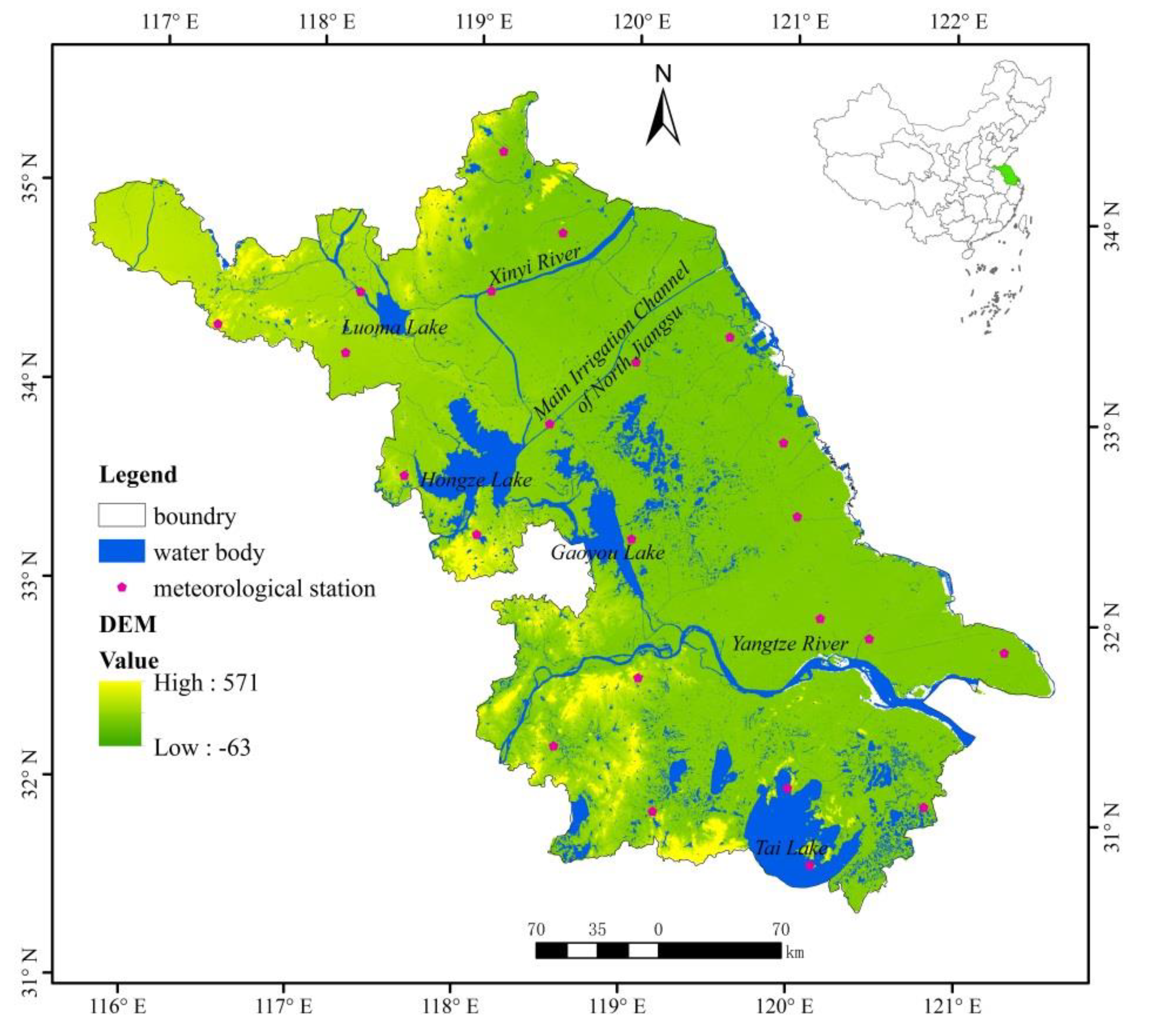
2.1. Study Area

Jiangsu Province (Figure 1) is located in the center of the eastern coast of mainland China, downstream on the Yangtze River (30°45′ to 35°20′ N; 116°18′ to 121°57′ E). The province mainly consists of plains, which account for more than 70% of the total area, and the lowest elevation is located at the Yangtze River estuary. Some low mountains and uplands are concentrated in the south-west and north-west. Additionally, there are dense networks of rivers, lakes and canals, such as Tai Lake, Hongze Lake, the Grand Canal and the Main Irrigation Channel of North Jiangsu (MICNJ), in the area. The annual rainfall totals approximately 850 mm [30]. The area south of the MICNJ is characterized by a subtropical humid monsoon climate, whereas the northern area has a warm temperate humid monsoon climate. There are 23 meteorological stations in the study area.

There are 13 cities in the study region, and the capital is Nanjing. In recent years, Jiangsu Province has led the country in comprehensive economic power. However, it is a resource-constrained province with acute contradictions associated with a high population and limited land. In 2001, Jiangsu Province proposed a plan for constructing an eco-province. The plan is divided into three periods (near-term 2005, medium-term 2010, and long-term 2020), and the framework of the eco-province is expected to be complete by 2020 [31]. Therefore, it is essential to evaluate ecological vulnerability and the factors that influence ecological vulnerability for sustainable socioeconomic development in Jiangsu Province in the short-term and medium-term planning time nodes, and 2015 was chosen as another reference year to maintain the 5-year interval.

2.2. Data Sources

The basic geographical data included administrative divisions vector data and a digital elevation model (DEM) with a resolution of 500 m.

The land use data included land use vector data from 2005, 2010 and 2015 that were produced via the artificial visual interpretation of Landsat thematic mapper (TM)/enhanced thematic mapper (ETM) image data. The land use classes include arable land, woodland, grassland, water bodies, built-up land, and unused land, with 6 types of upper-level classification, and the associated classification accuracy is greater than 94.3%. Additionally, 25 s-tier classifications are used, with the associated accuracy above 91.2% [32]. The land use classification system is shown in

Table 1. Land use classification system.

Upper-Level Classification		Second-Tier Classification
Code	Type	Code	Type
1	arable land	11	paddy field
		12	dry land
2	woodland	21	forest land
		22	shrubwood
		23	sparse woodland
		24	other woodland
3	grassland	31	high coverage grassland
		32	medium coverage grassland
		33	low coverage grassland
4	water body	41	canal
		42	lake
		43	reservoir pond
		44	permanent glacier snow
		45	coastal beach
		46	overflow land
5	built-up land	51	urban land
		52	rural settlements
		53	other construction land
6	unused land	61	sand
		62	gobi
		63	saline alkali land
		64	marsh land
		65	bare land
		66	bare rock and gravel land
		67	other unused land

, and the land use spatial distributions in Jiangsu Province are shown in Figure 2.

The normalized difference vegetation index (NDVI) data included the annual NDVI at a 1000-m resolution in 2005, 2010 and 2015.

The soil texture data were raster data of the sand, silt and clay percentages at a 1000-m resolution. These data were compiled from the 1:1,000,000 national soil type map and the second national soil survey data.

The meteorological data included the daily mean wind speed in winter and spring (December to May), daily mean rainfall and daily mean temperatures in 2005, 2010 and 2015 from 23 meteorological stations in Jiangsu Province (Figure 1).

The four types of data were derived from the Data Center for Resources and Environmental Sciences of the Chinese Academy of Sciences (RESDC) (http://www.resdc.cn), and these data have been widely used for research [33,34]. The meteorological data were obtained from the National Meteorological Science Data Sharing Service Platform (http://data.cma.cn/).

2.3. Methodology

2.3.1. Ecological Vulnerability Evaluation Index System

The ecological vulnerability evaluation index system based on land use, climate, topography and other data was established using the PSR model [17]. The system includes a target layer, a criterion layer and two index layers (

Table 2. Ecological vulnerability evaluation index system.

Target Layer	Criterion Layer	First-Level Indicator	Second-Level Indicator
	Pressure	Ecological sensitivity	Soil erosion sensitivity (ES)
			Soil desertification sensitivity (DS)
Ecological	State	Landscape pattern	Landscape patch density (PD)
vulnerability			Landscape evenness (SHEI)
	Response	Land resource utilization degree	Land resource utilization degree (LA)

).

The ecological sensitivity index, corresponding to the pressure layer, reflects the pressure of the ecological environment. The related second-level indicators include soil erosion sensitivity (ES) and soil desertification sensitivity (DS). The landscape pattern index, corresponding to the state layer, reflects the state of environmental quality, and landscape patch density (PD) and landscape evenness (SHEI) are the related second-level indicators. LA is the response of society to reduce the pressure on the environment through land use management measures, and LA corresponds to the response layer.

2.3.2. The Calculation of the Second-Level Indicators

The calculations and operation methods of the second-level indicators are shown in

Table 3. Calculation methods of the second-level indicators.

Second-Level Index	Description	Single Factor
		Factor	Formula	Operation
ES	Precipitation, topography, vegetation and soil factors, including rainfall erosivity (R), relief (LS), land use types (CM) and soil texture (ST), are used to evaluate ES using GIS technology. $ES=\sqrt[4]{{\displaystyle \prod }_{i=1}^4{C}_i}$, where $C_i$ is the sensitivity level of i.	R	$R={\displaystyle \sum _{i=1}^{12}\left(0.3046P_i-2.6398\right)}$. R is the annual rainfall erosivity (J·cm/m2·h); Pi is the monthly mean rainfall (mm) [35].	The monthly mean rainfall totals at 23 stations were calculated based on the daily mean rainfall. The R value at any station was then calculated, and the spatial distribution of R at a 1000-m resolution was obtained by the inverse distance weighted (IDW) interpolation method. Reclassification was performed according to Table 4 to obtain an R grade distribution map.
		LS	-	A 5 km × 5 km window analysis was conducted using the digital elevation model (DEM) to generate a LS spatial distribution map at a 500-m resolution. The map was then resampled to 1000 m using the nearest neighbor method. The reclassification to the LS grade distribution map was based on Table 4.
		CM	-	According to Table 4, the land use raster data were reclassified into a CM grade distribution map.
		ST	-	The ST spatial distribution was obtained from the integration of the raster data of the sand, silt and clay percentages with the con() function embedded in the raster calculator model of ArcGIS. This process was implemented according to the international grading standards for soil texture. The data were then reclassified to obtain an ST grade distribution map according to Table 4.
DS	DS was evaluated based on the vegetation coverage (C), moisture index (I), soil matrix (SM) and number of gale days (G) [36]. $DS=\sqrt[4]{{\displaystyle \prod }_{i=1}^4{D}_i}$, where $D_i$ is the sensitivity level of i.	C	$C=\frac{NDVI-NDV{I}_{min}}{NDV{I}_{max}-NDVI}$. NDVImin, NDVImax are the minimum and maximum of NDVI [37].	The C spatial distribution was calculated from the normalized difference vegetation index (NDVI) using the raster calculator in ArcGIS 10.2. The data were then reclassified to a C grade distribution map according to Table 4.
		I	$I=\frac{r}{0.16\sum t}$. $\sum t$ is the annual cumulative temperature not less than $10℃$; r is the annual rainfall during $t\ge 10 ℃$ [38].	The $\ge 10℃$ annual accumulated temperature was calculated based on the daily mean temperature at each station. The annual rainfall during the period of daily mean temperature $\ge 10℃$ was computed based on the daily mean rainfall. Then, the I value at any station was calculated and interpolated to obtain an I spatial distribution map at a 1000-m resolution. The reclassification to the I grade distribution map was performed according to Table 4.
		G	-	The number of days when the daily wind speed was greater than 6 m/s from December to May was determined for each meteorological station [39]. A G spatial distribution map at a 1000-m resolution was then obtained through IDW interpolation of the day numbers. Reclassification was performed to obtain a G grade distribution map according to Table 4.
		SM	-	According to Table 4, the ST spatial distribution was reclassified to an SM grade distribution map.
PD	-	PD	$PD=\frac{N}{A}$. N is the number of patches in the landscape unit; A is the area of landscape unit.	Grid method. A 1 km × 1 km fishnet was created and intersected with the land use vector data. Attribute statistics were obtained for the intersected data to determine N and A, and PD for each grid. The data table was joined to the fishnet, and the fishnet was rasterized with PD as the attribute value.
SHEI	SHEI equals the Shannon diversity index divided by the maximum possible diversity for a given landscape abundance. It can directly reflect the uneven distribution of patches, that is, landscape heterogeneity in a landscape system.	SHEI	$SHEI=\frac{-{\displaystyle \sum _{i=1}^{T}p\left(i\right)\ln \left(p\left(i\right)\right)}}{\ln \left(T\right)}$. p(i) is the area proportion of land use type i in a grid; T is the total number of land use types.	Grid method. The specific steps refer to the calculation of PD.
LA	-	LA	$LA=100\times {\displaystyle \sum _{i=1}^n{A}_i}\times C_i$. Ai is the land use degree grading index; Ci is the area proportion of level i in a grid. Land use degree grading standard is shown in Table 5.	Grid method. The specific steps refer to the calculation of PD. The land use degree grading standards refer to Zhuang and Liu [40].

.

Table 4. Sensitivity classification of the ecological sensitivity index [36,41].

Factor	Slight Sensitivity	Light Sensitivity	Medium Sensitivity	Heavy Sensitivity	Extreme Sensitivity
R	<25	25–100	100–400	400–600	>600
LS	<20	20–50	50–100	100–300	>300
CM	Water, swamp, paddy field	Broadleaf forest, coniferous forest, meadow, shrub and coppice forests	Sparse woods grassland, garden, dry land	Desert, settlements, sparse grassland	No vegetation area, bare land
ST	Gravel	Loamy sand	Sandy loam, sandy clay, sandy clay loam	Loam, clay loam, loam clay	Silty loam, silty clay loam, clay, silty clay
C	>0.7	0.5–0.7	0.3–0.5	0.1–0.3	<0.1
I	>0.65	0.5–0.65	0.2–0.5	0.05–0.2	<0.05
G	<15	15–30	30–45	45–60	>60
SM	Pedestal rock	Viscidity	Gravel	Loamy texture	Sandiness
Value	1	3	5	7	9

shows the sensitivity classification of the ecological sensitivity index. This process was conducted using ArcGIS10.2 (ESRI Inc., Redlands, CA, USA).

2.3.3. Index Standardization and the Determination of Weights

(1) Index Standardization

Positive indicators include ES, DS, PD and SHEI. LA is a negative indicator. The formulas of positive and negative indicators are shown as the following Formulas (1) and (2):

$$A_i=\frac{x_i-x_{min}}{x_{max}-x_{min}}$$

(1)

$$A_i=1-\frac{x_i-x_{min}}{x_{max}-x_{min}}$$

(2)

where A_i is the standardized value of indicator $x_i$; and $x_{max}$ and $x_{min}$ represent the maximum and minimum values of $x_i$, respectively.

(2) Determination of Weights

Using a rotating coordinate system, SPCA can transform raw variables into fewer independent composite variables and effectively reflect the original information [42].

Using the principal component module in ArcGIS, the eigenvector matrix of 5 s-level indicators and the contribution rates of principal components were obtained. The number of principal factors was 3 according to the principle that the cumulative contribution rate reaches 85%. Then, the common factor variance ($H_i$) of each second-level indicator was calculated based on Formula (3), and the weights ($W_i$) of the second-level indicators in 2005, 2010 and 2015 were further calculated (

Table 6. Weights of the second-level indicators in 2005, 2010 and 2015.

Index	Weight
	2005	2010	2015
ES	0.325	0.333	0.328
DS	0.286	0.107	0.289
PD	0.075	0.058	0.053
SHEI	0.258	0.277	0.281
LA	0.056	0.225	0.049

) using Formula (4):

$$H_i={\displaystyle \sum }_{k=1}^3{\lambda }_{ik}^2 \left(i=1, 2, 3, 4, 5\right)$$

(3)

where ${}_{ik}$ is the eigenvalue of second-level indicator i with respect to the principal component k.

$$W_i=H_i/{\displaystyle \sum }_{i=1}^5{H}_i$$

(4)

2.3.4. Ecological Vulnerability Grading Standard

Ecological vulnerability was obtained by the weighted summation of the second-level indicators. The results were divided into five grades by the natural breaks method. To keep the ecological vulnerability in the three years at the same grading standard, the mean values of the grading standards for the three years were taken as the final grading standard, namely, slight vulnerability: <0.1497; light vulnerability: 0.1498–0.2399; medium vulnerability: 0.2400–0.3247; heavy vulnerability: 0.3248–0.4339; and extreme vulnerability: >0.4339.

2.3.5. Spatial Autocorrelation Analysis

Spatial autocorrelation analysis, including global spatial autocorrelation and local spatial autocorrelation analyses, can reveal spatial scattering and clustering characteristics [43].

Global spatial autocorrelation reflects the overall spatial relationship and is usually represented by the Global Moran’s I index (I):

$$I=\frac{n{{\displaystyle \sum }}_{i=1}^n{{\displaystyle \sum }}_{j=1}^n{w}_{ij}\left(x_i-\overline{x}\right)\left(x_j-\overline{x}\right)}{{{\displaystyle \sum }}_{i=1}^n{{\displaystyle \sum }}_{j=1}^n{w}_{ij}{\left(x_i-\overline{x}\right)}^2}$$

(5)

where n is the number of grids; x_i and x_j are the values of grids i and j, respectively; $\overline{x}$ is the mean value of x; and w_ij is the spatial weight of grids i and j. When grid i is adjacent to grid j, w_ij = 1; otherwise, w_ij = 0. The range of I is [−1, 1]. If I > 0, the spatial correlation is positive. If I < 0, the spatial correlation is negative. Additionally, if I = 0, the spatial correlation is random.

The local spatial autocorrelation measures the correlation of adjacent regions, usually based on the local indicator of spatial association (LISA). According to the LISA, the study area was divided into five regions: (i) high–high (HH) regions, the region itself and its adjacent areas both have high ecological vulnerability; (ii) low–low (LL) regions, the ecological vulnerability of the region itself and its adjacent areas are low; (iii) low–high (LH) regions, the vulnerability of the region itself is low, with high vulnerability in the adjacent areas; (iv) high–low (HL) regions, the vulnerability of the region itself is high, and that of the surrounding areas is low; and (v) non-significant regions. There are spatial positive correlations in the HH and LL regions, negative correlations in the HL and LH regions, and no significant correlations in the non-significant regions.

This work was performed at the kilometer grid scale using OpenGeoda0.9.9.14 software.

2.3.6. Correlation Analysis

Three thousand random points were established in the study area. Five second-level indicators and the target layer were extracted to these points in ArcGIS. Then, simple correlation and partial correlation analyses between ecological vulnerability (x) and the second-level indicators (y, z ……) were conducted in SPSS19.0 (IBM Inc., Armonk, NY, USA):

$$r_{xy}=\frac{{{\displaystyle \sum }}_{i=1}^n\left(x_i-\overline{x}\right)\left(y_i-\overline{y}\right)}{\sqrt{{{\displaystyle \sum }}_{i=1}^n{\left(x_i-\overline{x}\right)}^2{{\displaystyle \sum }}_{i=1}^n{\left(y_i-\overline{y}\right)}^2}}$$

(6)

$$r_{xy,z}=\frac{r_{xy}-r_{xz}{r}_{yz}}{\sqrt{\left(1-r_{xz}{}^2\right)\left(1-r_{yz}{}^2\right)}}$$

(7)

where $r_{xy}$, $r_{xz}$, and $r_{yz}$ are the simple correlation coefficients of x and y, x and z, and y and z, respectively; $\overline{x}\mathrm{and}\overline{y}$ are mean values of x and y; $x_i\mathrm{and}{y}_i$ are the values of x and y at point i; and $r_{xy,z}$ is the partial correlation coefficient of x and y when z is controlled.

3. Results

3.1. Spatiotemporal Distribution of Ecological Vulnerability

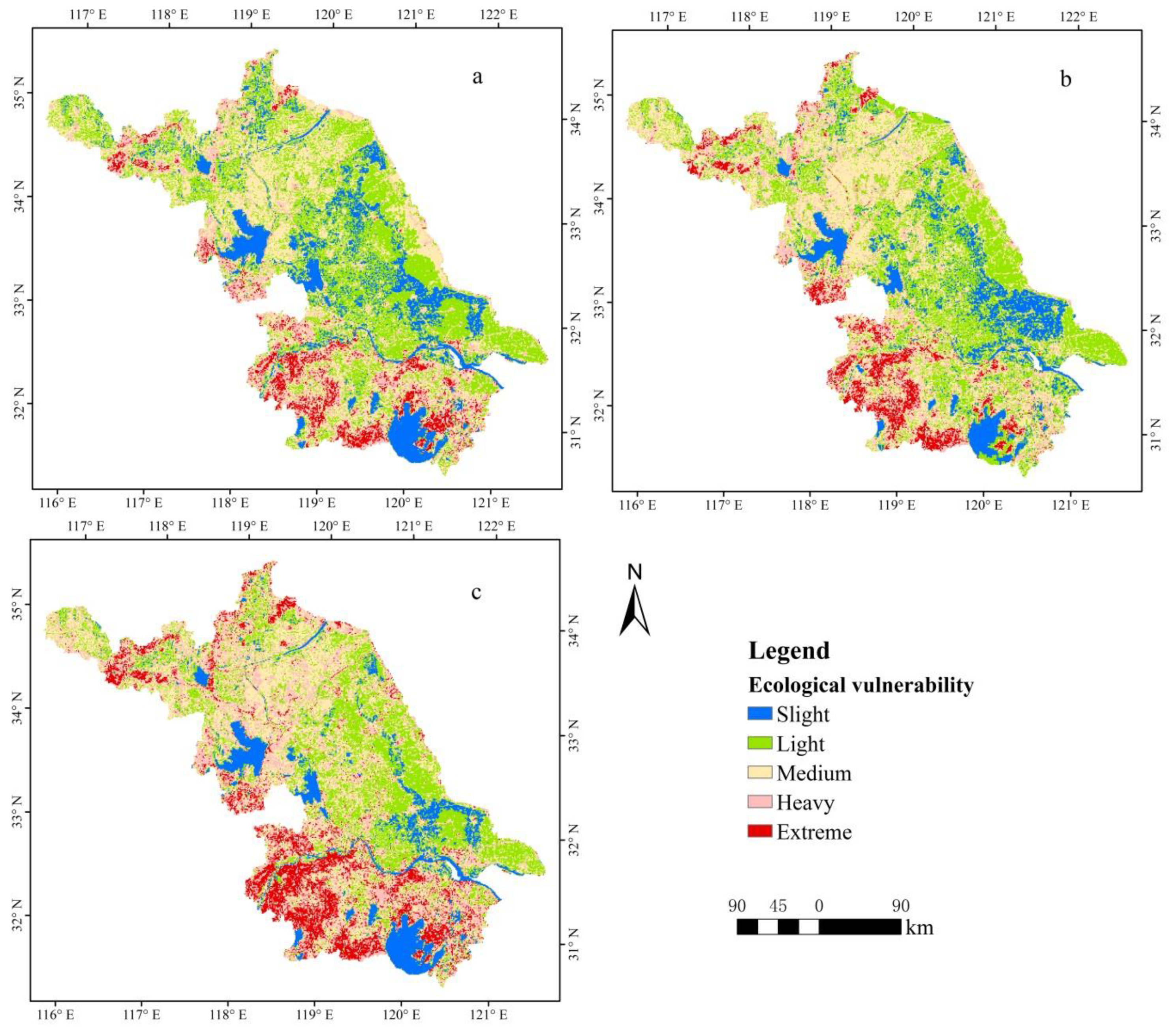
3.1.1. Spatial Distribution of Ecological Vulnerability

The mean values of ecological vulnerabilities in 2005, 2010 and 2015 were 0.267 ± 0.107, which is within the range of medium vulnerability. Most parts of Jiangsu Province exhibited light and medium ecological vulnerability, and the area combined proportions of light and medium vulnerability in 2005, 2010 and 2015 were 65%, 66.2% and 55.2%, respectively (Figure 3). Therefore, Jiangsu Province is overall lightly to moderately vulnerable.

As shown in Figure 4 and Figure 5, slight vulnerability accounts for 10% to 15% of the study area. These areas mainly include lakes, canals and some central paddy fields and comprise 66% to 85% of all lakes.

Light vulnerability accounts for approximately 1/3 of the study area. These areas are widely distributed in plain regions concentrated between the MICNJ and the Yangtze River. Arable land accounts for 74% to 86% of this vulnerability class, and the area of paddy fields is approximately 2.5 times that of dry land. In the study area, approximately 39% to 47% of the paddy fields are lightly vulnerable.

Medium vulnerability accounts for approximately 1/3 of the study area. These areas are concentrated to the north of the MICNJ and are mainly composed of arable and built-up land. Arable land accounts for 63% to 69% of this vulnerability class, encompassing 40% to 44% of the dry land in the study area. Built-up land occupies 23% to 26% of this class, covering 40% to 50% of the rural settlements in the study area.

Heavy vulnerability accounts for 15% to 25% of the study area. These areas are scattered to the south of the Yangtze River and in north-western hilly areas. Overall, 52% to 54% of the heavy vulnerability areas is arable land, and 25% to 34% is built-up land. This vulnerability class covers 39% to 47% of the woodland and approximately 34% of the grassland in the study area.

The proportion of extreme vulnerability is 6% to 12%. These areas concentrated in mountainous and hilly areas and mainly consist of arable land, built-up land and woodland. Moreover, this vulnerability class covers 56% to 79% of the unused land and 33% to 54% of the woodland in the study area.

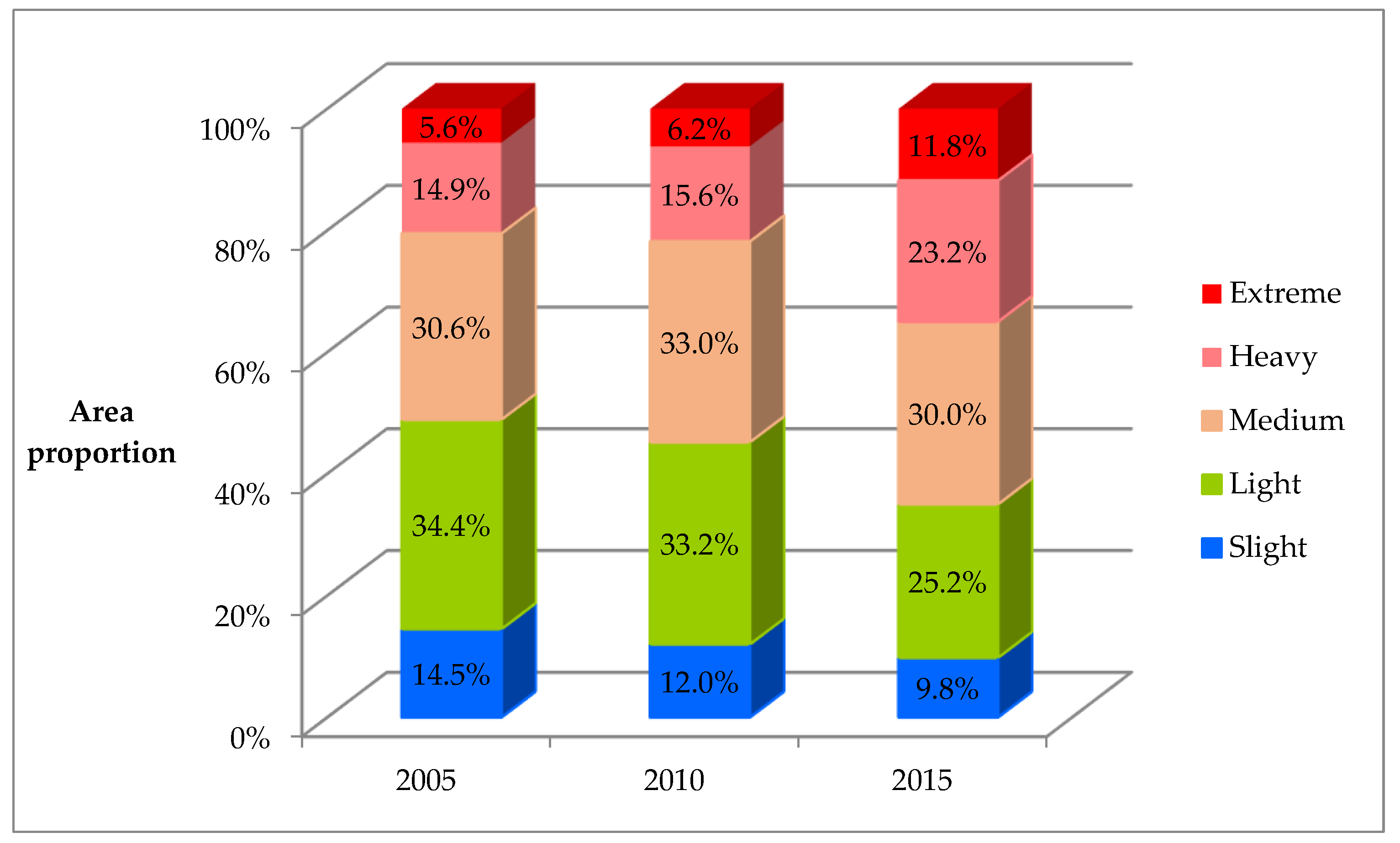
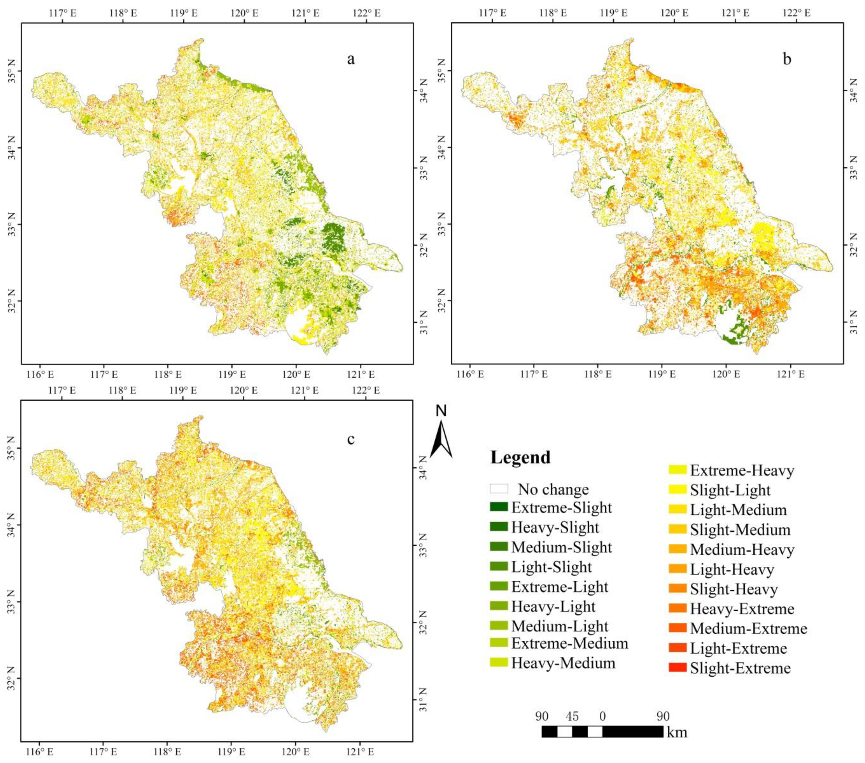
3.1.2. Temporal Variations in Ecological Vulnerability

The mean values of ecological vulnerability in 2005, 2010 and 2015 were 0.250 ± 0.103, 0.263 ± 0.097 and 0.288 ± 0.121, respectively. The increasing trend indicates a rise in vulnerability. In addition, the areal proportions of slight and light vulnerability constantly decreased, the medium vulnerability proportion initially increased and then decreased, and the proportions of heavy and extreme vulnerability increased steadily (Figure 3). Therefore, the ecological vulnerability gradually worsened.

From 2005 to 2010, the regions with unchanged ecological vulnerability accounted for 57.1% of the study area (Figure 6 and Figure 7). Areas with decreased ecological vulnerability accounted for 17.2% of the area. Approximately 55% of these areas were concentrated in the east-central coastal region of arable land, and 38% were located in built-up land areas along the north-eastern coast and in urban land areas. Areas with increased ecological vulnerability accounted for 25.7% of the study area. Notably, 60% of these areas were associated with north-western arable land, 18% with reservoirs and the borders of rivers and lakes, and approximately 10% with rural settlements. In hilly areas at high altitudes, the increase in vulnerability was obvious.

From 2010 to 2015, the areas where the ecological vulnerability level remained unchanged accounted for 60.4% of the total area. The ecological vulnerability level decreased in only 7% of the study area. Approximately 50% of the decreased regions were located at the borders of rivers and lakes, and the remainder was scattered in the arable land areas of the plains. Areas with increased ecological vulnerability accounted for 32.6% of the total area, of which approximately 60% were concentrated in arable land regions, especially in the central and southern paddy fields, and the remainder was associated with built-up land. The vulnerability of the built-up land along the north-eastern coast and the urban land areas increased significantly.

From 2005 to 2015, the regions with unchanged ecological vulnerability accounted for 51.8% of the study area. The ecological vulnerability level decreased in 7.9% of the study area. Approximately 59% of the decreased regions were scattered in arable land areas, forming small clusters in the dry land zone on the eastern coast and the paddy fields to the north-west of Hongze Lake. Additionally, 24% of the decreased regions were distributed in the urban land areas of the Yangtze River estuary. Areas with increased ecological vulnerability accounted for 20% of the total area. Sixty-four percent of the increased regions were concentrated in the arable land areas in the north-west, where the paddy field area is 2.4 times that of dry land. Moreover, approximately 24% of the increased regions were distributed in built-up land areas. In the north-western and southwestern hilly areas, the increase in vulnerability was particularly evident.

3.2. Autocorrelation Characteristics of Ecological Vulnerability

3.2.1. Global Spatial Autocorrelation

The Moran’s I values of ecological vulnerability in 2005, 2010 and 2015 were 0.7302, 0.7084 and 0.7169, respectively. These results indicate that ecological vulnerability exhibited a clustering characteristic. From 2005 to 2015, the overall cluster tendency first decreased and then slightly increased.

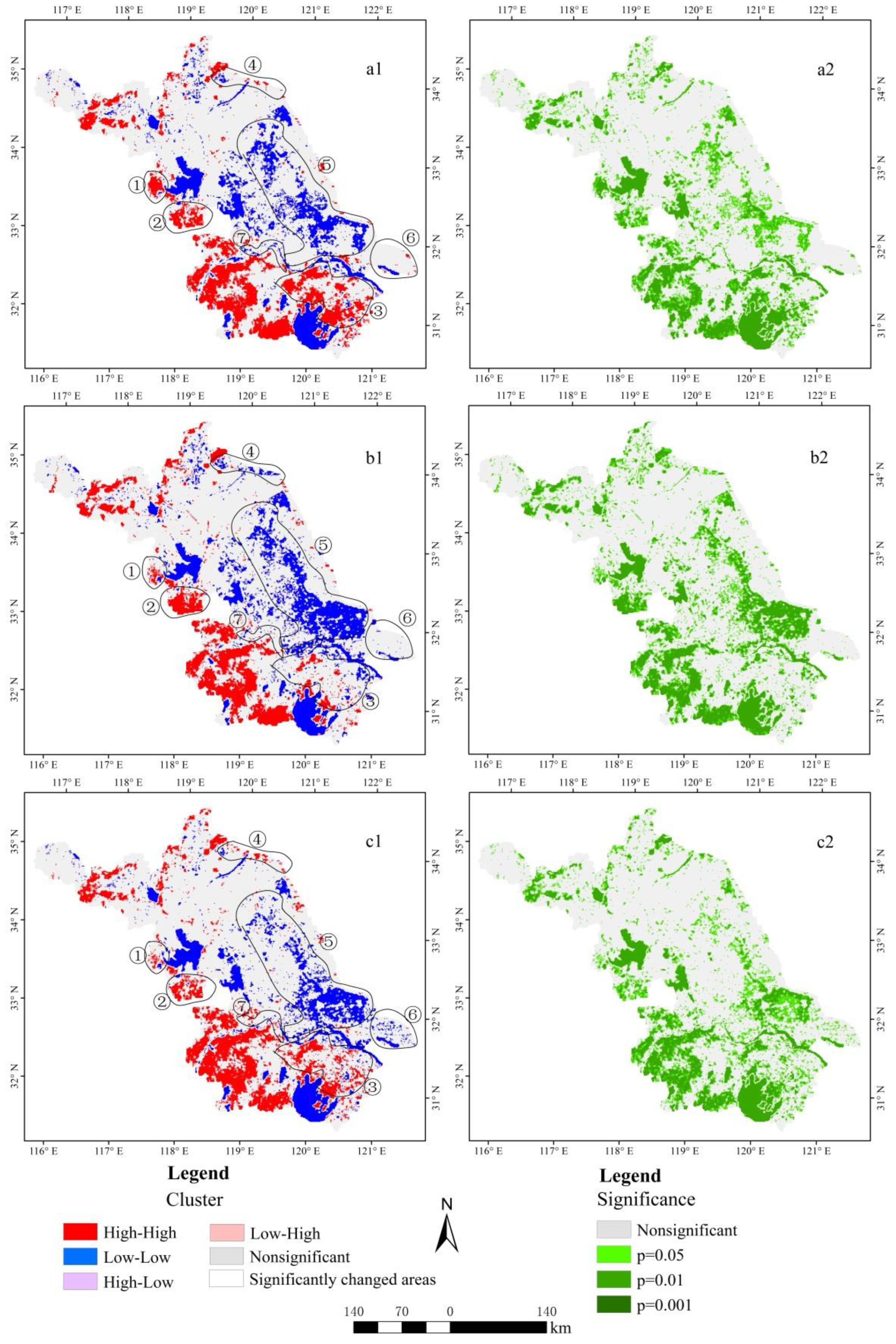
3.2.2. Local Spatial Autocorrelation

The spatial autocorrelation yielded similar distributions in 2005, 2010 and 2015 (Figure 8). HH areas were mainly distributed in regions with heavy or extreme vulnerability and concentrated in the urban land to the south of the Yangtze River and the western hills and mountains. From 2005 to 2015, the HH regions in ③ (Figure 8), the urban land to the south of the Yangtze River, and ④, the built-up land along the north-eastern coast, initially decreased and then increased. Additionally, the HH region in ①, the hilly area to the west of Hongze Lake, gradually decreased, and that in ②, the hilly area to the south-west of Hongze Lake, first increased and then decreased in area. The LL regions were mainly distributed in slight vulnerability areas, which were concentrated near water bodies. From 2005 to 2015, the LL area in ⑤, the eastern coastal paddy fields, first increased and then decreased; the LL area in ⑦, the middle section of the Yangtze River, first decreased and then increased; and the LL area in ⑥, the dry land area of the Yangtze River estuary, gradually increased. Moreover, the HH and LL autocorrelations in 2005, 2010 and 2015 generally reached 0.05 or 0.01 significance levels. The HL and LH regions were scattered in the study area.

3.3. Effects of Natural and Anthropogenic Factors on Ecological Vulnerability

The simple correlation and partial correlation results for the second-level indicators and ecological vulnerability are shown in

Table 7. The simple correlation results for the second-level indicators and ecological vulnerability.

2005
Indicator	Vulnerability	ES	DS	PD	SHEI	LA
vulnerability	1	0.523 **	0.047 **	0.791 **	0.797 **	0.754 **
ES		1	−0.001	0.456 **	0.396 **	0.568 **
DS			1	−0.040 *	−0.035	−0.014
PD				1	0.838 **	0.643 **
SHEI					1	0.525 **
LA						1
2010
Indicator	Vulnerability	ES	DS	PD	SHEI	LA
Vulnerability	1	0.534 **	0.074 **	0.813 **	0.828 **	0.741 **
ES		1	0.079 **	0.420 **	0.376 **	0.542 **
DS			1	0.074 **	0.051 **	0.051 **
PD				1	0.847 **	0.632 **
SHEI					1	0.518 **
LA						1
2015
Indicator	Vulnerability	ES	DS	PD	SHEI	LA
Vulnerability	1	0.505 **	0.088 **	0.789 **	0.783 **	0.776 **
ES		1	0.091 **	0.421 **	0.370 **	0.538 **
DS			1	0.079 **	0.048 **	0.060 **
PD				1	0.846 **	0.635 **
SHEI					1	0.515 **
LA						1

* indicates a significant correlation at the 0.05 level; ** indicates a significant correlation at the 0.01 level.

and

Table 8. The partial correlation results for the second-level indicators and ecological vulnerability.

Ecological Vulnerability (year)	ES	DS	PD	SHEI	LA
Vulnerability (2005)	0.102 **	0.164 **	0.129 **	0.497 **	0.535 **
Vulnerability (2010)	0.207 **	0.031	0.137 **	0.548 **	0.512 **
Vulnerability (2015)	0.097 *	0.06 **	0.112 **	0.472 **	0.593 **

* indicates a significant correlation at the 0.05 level; ** indicates a significant correlation at the 0.01 level.

.

Five second-level factors were significantly correlated with ecological vulnerability at the 0.01 level (Table 7). The correlation coefficients of PD, SHEI, LA and ecological vulnerability were the largest, followed by the correlation coefficient of ES and ecological vulnerability. The correlation coefficient of DS and ecological vulnerability was a minimum. ES and DS represent natural factors, and PD, SHEI and LA are anthropogenic factors. Therefore, the effects of anthropogenic factors on the ecological vulnerability were greater than those of natural factors. In addition, PD, SHEI and LA were moderately or highly positively correlated with each other, with correlation coefficients greater than 0.5. Notably, the correlation coefficient of PD and SHEI was 0.84. ES was moderately or slightly correlated with PD, SHEI and LA, with correlation coefficients ranging from 0.37 to 0.57.

The partial correlation coefficients between natural factors and ecological vulnerability did not exceed 0.25 (Table 8), so the natural factors had little effect on ecological vulnerability. The correlation between PD and ecological vulnerability was weak. SHEI and LA were moderately significantly positively correlated with ecological vulnerability, with partial correlation coefficients of approximately 0.5. Therefore, SHEI and LA are the main factors that influence ecological vulnerability.

4. Discussion

The natural conditions, such as climate and topography, in Jiangsu Province are superior, resulting in natural factors having little effect on ecological vulnerability. In recent years, rapid socioeconomic development in Jiangsu Province has led to changes in the ecological environment due to human activities. Land use, as an intuitive reflection of human activities, has a direct impact on ecological vulnerability [44]. The SHEI is a sensitive index that encompasses landscape heterogeneity. The higher the SHEI value is, the more complex the land use structure and the higher the fragmentation degree, then the greater the uncertainty of information, the more unstable the ecological system, and the greater the ecological vulnerability. LA refers to the human activities on the environment by modifying the structure of land use to mitigate and prevent their negative effects, based on an understanding of the ecological functions and values of different land use types. Therefore, as manifestations of land use, the SHEI and LA are the main factors that affect ecological vulnerability in the study area.

Slight vulnerability areas were mainly composed of water bodies. This result is related to the low SHEI and LA values of water bodies and is consistent with the findings of Qiao [45]. Light and medium vulnerability areas were concentrated in the arable lands of the plains, and these results are consisted with those of Fan et al. [46]. Specifically, the results are related to the effects of arable land on the composition and configuration of the landscape pattern [20]. Heavy and extreme vulnerability areas were mainly located in urban land areas and at high elevations. These results are associated with the high intensity of human activities in urban areas and the difficulty of environmental rehabilitation after disturbance at high elevations [3].

Ecological vulnerability gradually increased from 2005 to 2015. This result is consistent with the following actual conditions in Jiangsu Province.

(1)

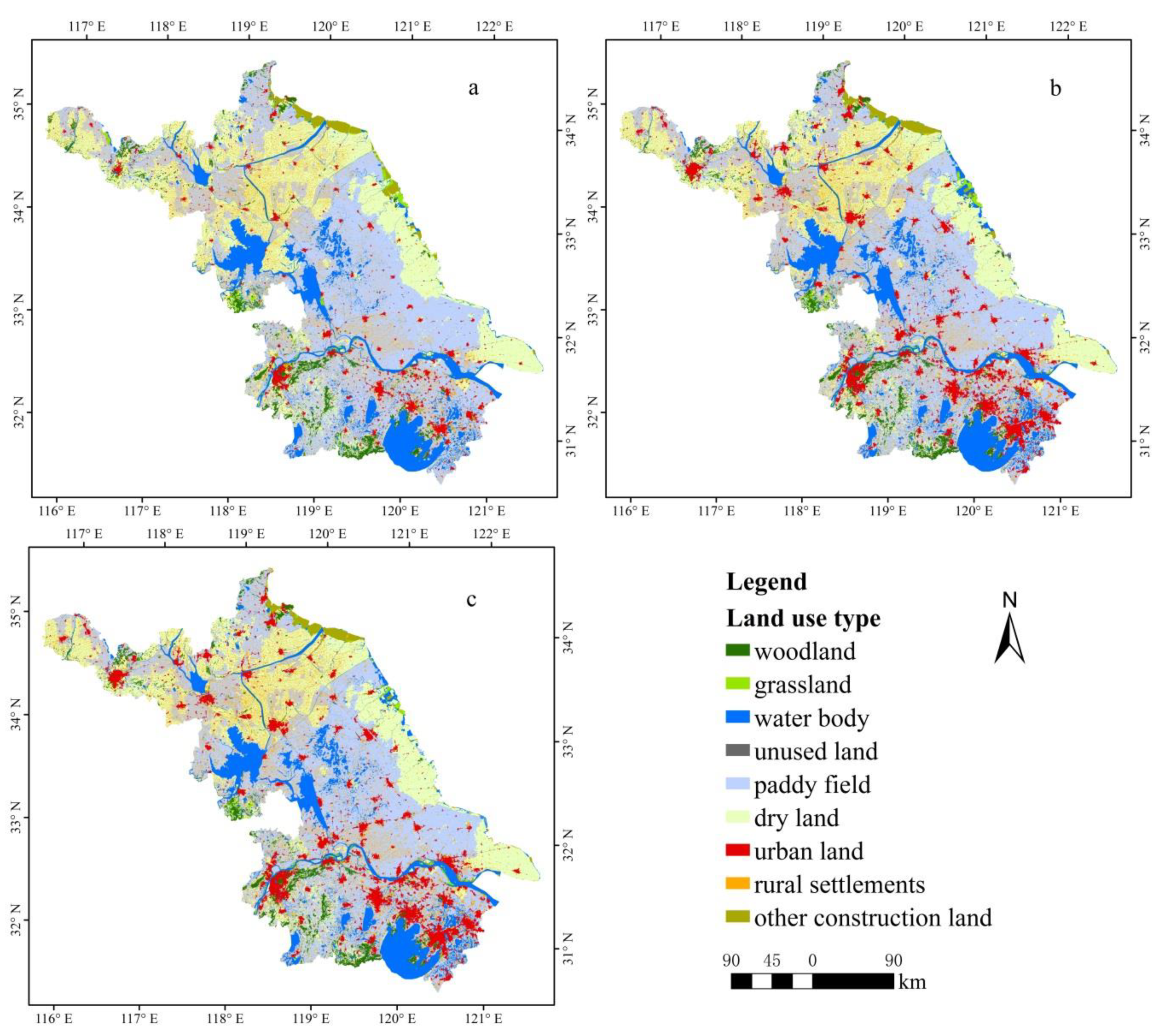
The arable land area declined from 68,363.91 km² in 2005 to 63,752.40 km² in 2010 and 62,921.95 km² in 2015, with a net decrease of 4611.51 km² from 2005 to 2010 and 830.45 km² from 2010 to 2015. In both phases, arable land was mainly converted to built-up land, accounting for 8.09% of arable land in 2005 and 7.05% in 2010. The reduction in arable land led to a more complex issue involving human activities and land use and management.

(2)

The woodland area decreased from 3352.49 km² in 2005 to 3098.42 km² in 2010 and 3049.91 km² in 2015, with a net decrease of 254.07 km² from 2005 to 2010 and 48.51 km² from 2010 to 2015. From 2005 to 2015, the reclaimed area reached 195.57 km² and accounted for 52.74% of the decreased area of woodlands. Reclamation and cultivation can cause extensive hydrological changes and soil erosion and deterioration of the eco-environment [9].

(3)

The population in the study area increased from 75.8824 million in 2005 to 78.6934 million in 2010 and 79.7630 million in 2015 [47]. Hong et al. [48] showed that vulnerability is correlated with population agglomeration.

(4)

Economic development activities are fundamental factors that influence ecological vulnerability [49]. The gross industrial production in Jiangsu Province increased from 9440.18 billion in 2005 to 19,277.65 billion in 2010 and 27,996.43 billion in 2015 [47]. Moreover, the industrial and mining land areas continued to increase from 1416.28 km² in 2005 to 1421.05 km² in 2010 and 1497.04 km² in 2015, with a net increase of 4.77 km² from 2005 to 2010 and 75.99 km² from 2010 to 2015.

Additionally, an ecological vulnerability assessment index system was constructed in this study based on land use, and the spatial and temporal changes in the ecological vulnerability of Jiangsu Province were analyzed from the aspects of land use, climate, topography, soil and vegetation to explore the ecological vulnerability and the influence factors. Therefore, the study did not involve other human activity-related factors, such as industrialization and eutrophication, in addition to land use. The results of the ecological vulnerability assessment and the subsequent analysis are based on this premise.

5. Conclusions

This study assessed the spatiotemporal distribution and influence factors of ecological vulnerability in Jiangsu Province. The conclusions of the study are as follows.

(1)

The effects of anthropogenic factors on ecological vulnerability were greater than those of natural factors, and the SHEI and LA were the main factors that influence ecological vulnerability.

(2)

Most parts of Jiangsu Province exhibited light and medium ecological vulnerability. The areal proportions of different vulnerability levels sorted in descending order are as follows: light ≈ medium > heavy > slight > extreme. Slight vulnerability mainly included the areas of lakes and canals. Light vulnerability areas were mainly distributed in paddy fields between the MICNJ and the Yangtze River. Medium, heavy and extreme vulnerability areas were mainly composed of arable and built-up land. Medium vulnerability was concentrated to the north of the MICNJ; heavy vulnerability was scattered to the south of the Yangtze River and in north-western hilly areas; and extreme vulnerability was concentrated in hilly areas.

(3)

Ecological vulnerability displayed a clustering characteristic. HH areas were mainly distributed in heavy and extreme vulnerability regions, and LL regions were associated with slight vulnerability areas.

(4)

Ecological vulnerability gradually deteriorated in the study area. From 2005 to 2010, the vulnerability in hilly areas obviously increased, and from 2010 to 2015, the vulnerability in urban and north-eastern coastal built-up land areas significantly increased.

Therefore, emphasis should be placed on the prevention and control of ecological vulnerability in high-altitude, urban land and coastal areas. In high-altitude areas, deforestation should be strictly prevented from replacing with arable land and buildings. Funding should be available for forest fire mitigation as needed, and ecological restoration measures should be improved. In urban and coastal areas, an environmentally sound and sustainable economic compensation strategy should be established to regulate human activities.

References

1. Adger, W.N. Vulnerability. Glob. Environ. Chang. 2006, 16, 268–281. [Google Scholar] [CrossRef]
2. Wang, X.D.; Zhong, X.H.; Gao, P. A GIS-based decision support system for regional eco-security assessment and its application on the Tibetan Plateau. J. Environ. Manag. 2010, 91, 1981–1990. [Google Scholar] [CrossRef]
3. Zou, T.H.; Yoshino, K. Environmental vulnerability evaluation using a spatial principal components approach in the Daxing’anling region, China. Ecol. Indic. 2017, 78, 405–415. [Google Scholar] [CrossRef]
4. Hou, K.; Li, X.X.; Zhang, J. GIS analysis of changes in ecological vulnerability using a SPCA model in the Loess Plateau of Northern Shaanxi, China. Int. J. Environ. Res. Public Health 2015, 12, 4292–4305. [Google Scholar] [CrossRef] [PubMed]
5. Park, Y.S.; Chon, T.S.; Kwak, I.S.; Lek, S. Hierarchical community classification and assessment of aquatic ecosystems using artificial neural networks. Sci. Total Environ. 2004, 327, 105–122. [Google Scholar] [CrossRef] [PubMed]
6. Liu, D.; Cao, C.X.; Dubovyk, O.; Tian, R.; Chen, W.; Zhuang, Q.F.; Zhao, Y.J.; Menz, G. Using fuzzy analytic hierarchy process for spatio-temporal analysis of eco-environmental vulnerability change during 1990–2010 in Sanjiangyuan region, China. Ecol. Indic. 2017, 73, 612–625. [Google Scholar] [CrossRef]
7. Nguyen, A.K.; Liou, Y.A.; Li, M.H.; Tran, T.A. Zoning eco-environmental vulnerability for environmental management and protection. Ecol. Indic. 2016, 69, 100–117. [Google Scholar] [CrossRef]
8. Wang, Y.; Ding, Q.; Zhuang, D.F. An eco-city evaluation method based on spatial analysis technology: A case study of Jiangsu Province, China. Ecol. Indic. 2015, 58, 37–46. [Google Scholar] [CrossRef] [Green Version]
9. Shao, H.Y.; Liu, M.; Shao, Q.F.; Sun, X.F.; Wu, J.H.; Xiang, Z.Y.; Yang, W.N. Research on eco-environmental vulnerability evaluation of the Anning River Basin in the upper reaches of the Yangtze River. Environ. Earth Sci. 2014, 72, 1555–1568. [Google Scholar] [CrossRef]
10. Bhuiyan, J.A.N.; Dutta, D. Analysis of flood vulnerability and assessment of the impacts in coastal zones of Bangladesh due to potential sea-level rise. Nat. Hazards 2012, 61, 729–743. [Google Scholar] [CrossRef]
11. Cao, C.X.; Yang, B.; Xu, M.; Li, X.W.; Singh, R.P.; Zhao, X.J.; Chen, W. Evaluation and analysis of post-seismic restoration of ecological security in Wenchuan using remote sensing and GIS. Geomat. Nat. Hazards Risk 2016, 7, 1919–1936. [Google Scholar] [CrossRef]
12. Martins, V.N.; Silva, D.S.; Cabral, P. Social vulnerability assessment to seismic risk using multicriteria analysis: The case study of Vila Franca do Campo (Sao Miguel Island, Azores, Portugal). Nat. Hazards 2012, 62, 385–404. [Google Scholar] [CrossRef]
13. Eckert, S. Remote sensing-based assessment of tsunami vulnerability and risk in Alexandria, Egypt. Appl. Geogr. 2012, 32, 714–723. [Google Scholar] [CrossRef]
14. Bosom, E.; Jimenez, J.A. Probabilistic coastal vulnerability assessment to storms at regional scale-application to Catalan beaches (NW Mediterranean). Nat. Hazards Earth Syst. Sci. 2011, 11, 475–484. [Google Scholar] [CrossRef] [Green Version]
15. Buxton, M. Vulnerability to bushfire risk at Melbourne’s urban fringe: The failure of regulatory land use planning. Geogr. Res. 2011, 49, 1–12. [Google Scholar] [CrossRef]
16. Pei, H.; Fang, S.F.; Lin, L.; Qin, Z.H.; Wang, X.Y. Methods and applications for ecological vulnerability evaluation in a hyper-arid oasis: A case study of the Turpan Oasis, China. Environ. Earth Sci. 2015, 74, 1449–1461. [Google Scholar] [CrossRef]
17. Qiao, Z.; Yang, X.; Liu, J.; Xu, X.L. Ecological vulnerability assessment integrating the spatial analysis technology with algorithms: A case of the wood-grass ecotone of northeast China. Abstr. Appl. Anal. 2013, 2013, 1–8. [Google Scholar] [CrossRef]
18. Song, G.B.; Chen, Y.; Tian, M.R.; Lv, S.H.; Zhang, S.S.; Liu, S.L. The Ecological Vulnerability Evaluation in Southwestern Mountain Region of China Based on GIS and AHP Method. Procedia Environ. Sci. 2010, 2, 465–475. [Google Scholar] [CrossRef] [Green Version]
19. Ma, J.; Li, C.X.; Wei, H.; Ma, P.; Yang, Y.J.; Ren, Q.S.; Zhang, W. Assessment of ecological vulnerability in three Gorges area. Acta Ecol. Sin. 2015, 35, 1–13. [Google Scholar] [CrossRef]
20. Aretano, R.; Semeraro, T.; Petrosillo, T.; Marco, A.D.; Pasimeni, M.R.; Zurlini, G. Mapping ecological vulnerability to fire for effective conservation management of natural protected areas. Ecol. Model. 2014, 295, 163–175. [Google Scholar] [CrossRef]
21. Valois, C.H.; Martínez, R.C. Vulnerability of native forests in the Colombian Chocó: Mining and biodiversity conservation. Bosque 2016, 37, 295–305. [Google Scholar] [CrossRef]
22. Yang, Y.J.; Ren, X.F.; Zhang, S.L.; Chen, F.; Hou, H.P. Incorporating ecological vulnerability assessment into rehabilitation planning for a post-mining area. Environ. Earth Sci. 2017, 76, 245. [Google Scholar] [CrossRef]
23. Bárcena, J.F.; Gómez, A.G.; García, A.; Álvarez, C.; Juanes, J.A. Quantifying and mapping the vulnerability of estuaries to point-source pollution using a multi-metric assessment: The Estuarine Vulnerability Index (EVI). Ecol. Indic. 2017, 76, 159–169. [Google Scholar] [CrossRef]
24. Malekmohammadi, B.; Jahanishaki, F. Vulnerability assessment of wetland landscape ecosystem services using driver-pressure-state-impact-response (DPSIR) model. Ecol. Indic. 2017, 82, 293–303. [Google Scholar] [CrossRef]
25. Parthasarathy, A.; Natesan, U. Coastal vulnerability assessment: A case study on erosion and coastal change along Tuticorin, Gulf of Mannar. Nat. Hazards 2014, 75, 1713–1729. [Google Scholar] [CrossRef]
26. Tapia, C.; Abajo, B.; Feliu, E.; Mendizabal, M.; Martinez, J.A.; Fernández, J.G.; Laburu, T.; Lejarazu, A. Profiling urban vulnerabilities to climate change: An indicator-based vulnerability assessment for European cities. Ecol. Indic. 2017, 78, 142–155. [Google Scholar] [CrossRef]
27. Zhang, X.R.; Wang, Z.B.; Lin, J. GIS Based Measurement and Regulatory Zoning of Urban Ecological Vulnerability. Sustainability 2015, 7, 9924–9942. [Google Scholar] [CrossRef] [Green Version]
28. Pearson, L.J.; Nelson, R.; Crimp, S.; Langridge, J. Interpretive review of conceptual frameworks and research models that inform Australia’s agricul-tural vulnerability to climate change. Environ. Model. Softw. 2011, 26, 113–123. [Google Scholar] [CrossRef]
29. Li, Y.; Tang, G.A.; Yang, G.; Li, Y. Research progress of ecological vulnerability based on metrological analysis of literatures in China. J. Hunan Univ. Sci. Technol. 2012, 15, 91–94. [Google Scholar]
30. Xu, C.G.; Feng, X.F.; Zheng, Z.W.; Shen, Z.T. Study on Characteristics for Spatial and Temporal Distribution in Jiangsu Province. Mod. Agric. Sci. Technol. 2014, 20, 236–239. [Google Scholar]
31. Tan, J.H.; Tang, M.L. The theory of ecological footprint and the eco-province construction of Jiangsu. J. Nanjing Norm. Univ. 2006, 29, 121–126. [Google Scholar]
32. Liu, J.Y.; Kuang, W.H.; Zhang, Z.X.; Xu, X.L.; Qin, Y.W.; Ning, J.; Zhou, W.S.; Zhang, S.W.; Li, R.D.; Yan, C.Z.; et al. Spatiaotemporal characteristics, patterns and causes of land-use changes in China since the late 1980s. J. Geogr. Sci. 2014, 24, 195–210. [Google Scholar] [CrossRef]
33. Ding, Q.; Cheng, G.; Wang, Y.; Zhuang, D.F. Effects of natural factors on the spatial distribution of heavy metals in soils surrounding mining regions. Sci. Total Environ. 2017, 578, 577–585. [Google Scholar] [CrossRef] [PubMed]
34. Ji, W.; Wang, Y.; Zhuang, D.F.; Song, D.P.; Shen, X.; Wang, W.; Li, G. Spatial and temporal distribution of expressway and its relationships to land cover and population: A case study of Beijing, China. Transp. Res. D 2014, 32, 86–96. [Google Scholar] [CrossRef] [Green Version]
35. Zhou, F.J.; Chen, M.H.; Lin, F.X. R value of the indices of rainfall erosivity in Fujian province. J. Soil Water Conserv. 1995, 9, 13–18. [Google Scholar]
36. Office of the Leading Group for the Development of the Western Region of the State Council, State Environmental Protection Administration of China. The Ecological Function Division Interim Regulations; Office of the Leading Group for the Development of the Western Region of the State Council, State Environmental Protection Administration of China: Beijing, China, 2002.
37. Rouse, J.W.; Haas, R.W.; Schell, J.A.; Deering, D.W.; Harlan, J.C. Monitoring the Vernal Advancement and Retrogradation (Green Wave Effect) of Natural Vegetation; NASA: Washington, DC, USA, 1974.
38. Meng, M.; Ni, J.; Zhang, Z.G. Geographical ecology of aridity index and its application. J. Plant Ecol. 2004, 28, 853–861. [Google Scholar]
39. Zhang, G.P.; Zhang, Z.X.; Liu, J.Y. Analysis of spatial patterns and driving factors of soil wind erosion in China. Acta Geogr. Sin. 2001, 56, 146–158. [Google Scholar]
40. Zhuang, D.F.; Liu, J.Y. Study on the model of regional differentiation of land use degree in China. J. Nat. Resour. 1997, 12, 105–111. [Google Scholar]
41. Zhang, Z.Q.; Zhang, J.; Huang, G.B. Ecological sensitivity and managemental countermeasures of envrionments in Qingyang city, Gansu province. J. Desert Res. 2010, 30, 614–619. [Google Scholar]
42. Brejda, J.J.; Moorman, T.B.; Karlen, D.L.; Dao, T.H. Identification of regional soil quality factors and indicators: I. Central and southern high plain. Soil Sci. Soc. Am. 2000, 64, 2115–2124. [Google Scholar] [CrossRef]
43. Shi, H.; Yang, Z.P.; Han, F.; Shi, T.G.; Luan, F.M. Characteristics of temporal-spatial differences in landscape ecological security and the driving mechanism in Tianchi scenic zone of Xinjiang. Prog. Geogr. 2013, 32, 475–485. [Google Scholar] [CrossRef]
44. Zhao, Y.X.; Liu, X.; Qin, Y.J.; Xu, Q.H. LUCC and its impact on vulnerability of agro-pastoral areas in Hebei province. Res. Soil Water Conserv. 2011, 18, 205–211. [Google Scholar]
45. Qiao, Z. The Impact Assessment of Ecological Vulnerability Based on the Land-Use in the Transitional Area between Forest and Grass Regions in Northeast China. Master’s Thesis, Shandong Normal University, Jinan, China, 2011. [Google Scholar]
46. Fan, S.L.; Guo, Y.S.; Qiu, L.J.; Jiang, C.; Huang, Y.H. Analyzing the effects of land cover change on urban ecological vulnerability in the central districts of Fuzhou city. J. Fujian Norm. Univ. 2018, 34, 92–98. [Google Scholar] [CrossRef]
47. Jiangsu Statistical Yearbook. Available online: http://www.jssb.gov.cn/2016nj/indexc.htm (accessed on 29 August 2018).
48. Hong, W.; Jiang, R.R.; Yang, C.Y.; Zhang, F.F.; Su, M.; Liao, Q. Establishing an ecological vulnerability assessment indicator system for spatial recognition and management of ecologically vulnerable areas in highly urbanized regions: A case study of Shenzhen, China. Ecol. Indic. 2016, 69, 540–547. [Google Scholar] [CrossRef]
49. Lee, Y. Social vulnerability indicators as a sustainable planning tool. Environ. Impact Assess. 2014, 44, 31–42. [Google Scholar] [CrossRef]
Figure 1. The geographical environment of the study area.
Sustainability 10 03087 g001
Figure 2. Land use types in Jiangsu Province ((a) 2005; (b) 2010; (c) 2015). To facilitate the analysis, the woodland, grassland, water body and unused land classes are displayed as upper-level classifications, and arable land and built-up land are shown with second-tier classifications. The second-tier classifications of arable land are paddy field and dry land. The second-tier classifications of built-up land are urban land, rural settlements and other construction land.
Sustainability 10 03087 g002
Figure 3. Area proportions of different vulnerability levels in 2005, 2010 and 2015.
Sustainability 10 03087 g003
Figure 4. The spatial distributions of ecological vulnerability in Jiangsu Province ((a) 2005; (b) 2010; (c) 2015).
Sustainability 10 03087 g004
Figure 5. The area proportions of different land use types for the five ecological vulnerability levels in 2005, 2010 and 2015. ((a) slight vulnerability; (b) light vulnerability; (c) medium vulnerability; (d) heavy vulnerability; (e) extreme vulnerability).
Sustainability 10 03087 g005aSustainability 10 03087 g005b
Figure 6. Temporal variations in ecological vulnerability ((a) 2005–2010; (b) 2010–2015; (c) 2005–2015).
Sustainability 10 03087 g006
Figure 7. Areal properties of different land use types in regions where ecological vulnerability increased, decreased or did not change ((a) 2005–2010; (b) 2010–2015; (c) 2005–2015).
Sustainability 10 03087 g007
Figure 8. Local spatial autocorrelation diagrams (the left three figures. (a1): 2005; (b1): 2010; (c1): 2015. ①②③④ are the areas where the high–high (HH) level changed significantly, and ⑤⑥⑦ are the areas where the low–low (LL) level changed significantly) and the significance test diagrams (the right three figures. (a2): 2005; (b2): 2010; (c2): 2015).
Sustainability 10 03087 g008