Prediction and Analysis of the Relationship between Energy Mix Structure and Electric Vehicles Holdings Based on Carbon Emission Reduction Constraint: A Case in the Beijing-Tianjin-Hebei Region, China

Abstract

In response to air pollution problems caused by carbon emissions, electric vehicles are widely promoted in China. Since thermal power generation is the main form of power generation, the large-scale development of electric vehicles is equivalent to replacing oil with coal, which will accordingly result in carbon emissions increasing if the scale of electric vehicles exceeds a certain limit. A relationship model between regional energy mix structure and electric vehicles holdings under the constraint of carbon emission reduction is established to perform a quantitative analysis of the limitation mechanism. In order to measure the scale of the future electric vehicle market under the constraint of carbon emissions reduction, a method called Extreme Learning Machine optimized by Improved Particle Swarm Optimization (IPSO-ELM) with higher precision than Extreme Learning Machine (ELM) is proposed to predict the power structure and the trend of electric vehicle development in the Beijing-Tianjin-Hebei region from 2019–2030. The calculation results show that the maximum number of electric vehicles must not exceed 19,340,000 and 26,867,171 based on emissions reduction aims and also the predicted energy mix structure in the Beijing-Tianjin-Hebei region in 2020 and 2030. At this time, the ratio of electric vehicles to traditional car ownership is 75.6% and 78.3%. The proportion of clean energy generation should reach 0.314 and 0.323 to match a complete replacement of traditional fuel vehicles for electric vehicles. A substantial increase in clean energy generation is needed so that the large-scale promotion of electric vehicles can still achieve the goal of carbon reduction. Therefore, this article will be helpful for policy-making on electric vehicle development scale and energy mix structure in the Beijing-Tianjin-Hebei region.

1. Introduction

The contradiction between the development of the economy and the environment has remained a huge challenge for decades. Energy conservation and emission reduction have been incorporated into national strategic planning. The transportation industry is considered to be a key industry for carbon emissions in many countries and the automobile industry is an important factor in oil consumption and carbon emissions. It puts great pressure on China’s carbon reduction commitment that “Carbon dioxide emissions per unit of GDP will fall by 40–50% from 2005 to 2020” [1]. Therefore, under the pressure of energy and environmental protection, new energy vehicles will undoubtedly become the main aspect of the automobile industry in China and electric vehicles with “low pollution,” “high energy conversion rate” and “evening low charging” have become the first choice for the transformation of new energy vehicles [2].

Compared with traditional fuel cars, electric vehicles have a big advantage in reducing emissions. In order to comprehensively compare the impact of electric vehicles on the environment compared with traditional fuel vehicles, extensive research has been carried by domestic and foreign scholars, which mainly involves the fuel life cycle, power system life cycle, related component life cycle and vehicle life cycle [3,4,5,6]. It is generally believed that the development of electric vehicles is more conducive to energy saving and emissions reduction than traditional vehicles. Siaoqing et al. compared the vehicles in the use phase and found that the electric vehicles have the advantages of low fossil energy consumption, high energy utilization efficiency and near-zero emissions during the driving process [7]. There are also scholars who compared electric cars and traditional cars from the perspective of the whole life cycle, from the power generation structure, vehicle fuel type [8], power generation energy structure, coal power technology power supply route [7], hybrid electric vehicle driving efficiency [9] and charging strategy [10] and found that the electric cars have different degrees of impact on carbon emissions during the production and power supply stages.

However, thermal power generation, regarded as the main form of power generation in China, causes large-scale electric vehicles to transfer carbon emissions to the power generation side. It is believed that the high-speed development of electric vehicles is equivalent to replacing oil with coal [11]. The conversion efficiency of coal into electric energy is about 45% and the conversion efficiency of petroleum into electric energy is about 65%. From the perspective of primary energy conversion efficiency, the conversion efficiency of coal is less than that of oil. As such, it is essential to study whether the large-scale development of electric vehicles can achieve carbon emission reduction. The carbon emissions of electric vehicles and the carbon emission measurement model have been extensively studied and analyzed by domestic and foreign scholars.

In terms of the carbon emissions of electric vehicles, Reed T. Doucette et al. compared carbon emissions models for hybrid and pure electric vehicles and compared existing carbon emissions from conventional vehicles [12]. The research results showed that plug-in hybrid vehicles have better carbon emission reduction potential for China’s high-density power generation countries. Patrick and Sonja et al. [13], using an optimized energy system model (PERSEUS-NET-TS), discussed four methods for assessing electric vehicles’ CO₂ emissions in Germany in 2030. It is found that different evaluation methods have great differences in the calculation results of CO₂ emissions and some of the results even exceed the emissions of internal combustion engines. Thiel et al. [14] compared carbon emissions in 2010 before the implementation of the new energy policy and 2030 after the implementation of the new energy policy in Europe based on the analysis of carbon emissions and the carbon emission reduction costs of traditional fuel vehicles, plug-in hybrid vehicles and pure electric vehicles in the European automotive market, which affirmed the positive impact of energy policy on carbon emission reduction. Nanaki et al. [15], who had studied the carbon emission capacity of hybrid and electric vehicles from the production, used phases of vehicles and found that the environmental impact of electric vehicles depends mainly on the power source. Shi Xiaoqing et al. [7] used an improved fuel carbon emission model and set up six scenarios to analyze the factors influencing promotion of pure electric vehicles in Beijing; they believed that the energy structure played a decisive role in the carbon emission reduction of pure electric vehicles. Huang Ying et al. [16] used the Economic Input-Output Life Cycle Assessment (EIO-LCA) method to analyze the greenhouse gas emissions of electric vehicles and traditional fuel vehicles and concluded that the main factor affecting the emission of greenhouse gases in electric vehicles is the production and supply of electricity, so it is necessary to optimize the energy structure.

In terms of the carbon emission measurement model, typical models of carbon emission estimation from home and abroad, such as the Logistic model, ERM-AIM model, MARKAL model and system dynamics measurement model are widely used. Machteld van den Broek et al. [17] used the MARKAL model to conduct a quantitative scenario study of the power and cogeneration industry through the analysis of factors such as carbon emissions, carbon abatement costs and carbon storage in the Netherlands, which enabled the prediction and assessment of strategies for achieving 15% and 50% carbon reduction in 2020 and 2050 at the 1990 level. Based on various factors, such as fuel price, promotion policy and technological development, J. Brady and M. O’Mahony [18] used the Logistics model to predict the different promotion effects of 2020 electric vehicle ownership and calculate carbon emissions. It is clear from the results that, from the perspective of long-term development, the widespread use of electric vehicles in urban transportation can significantly reduce CO₂ emissions; however, in a short period of time, the energy saving and emission reduction effects that can be achieved by promoting electric vehicles are limited. R.T. Doucette et al. compared the different energy structures of the United States, France and China with a carbon emission model for plug-in hybrid vehicles and concluded that, in the above circumstances, the emission reduction effects of plug-in hybrid vehicles in different countries are different and, considering the current status of coal-based power generation in China, the emission reduction effect that can be achieved by developing electric vehicles is relatively poor.

In summary, the existing literature only quantitatively analyzes the carbon emissions of electric vehicles. There is no further analysis and planning for the number of electric vehicles in combination with the number of traditional vehicles in response to China’s carbon emission reduction targets.

Therefore, based on the previous literature and comprehensive utilization, this paper calculated the maximum quantity of electric vehicles in the Beijing-Tianjin-Hebei region in 2020 and 2030 against a background of carbon emission reduction with the prediction of the energy mix structure of 2018–2030 and a model of a correlational relationship between energy mix structure and electric vehicle holdings. In order to ensure a balance between energy supply and demand and reduce the gap between them, the prediction of the energy mix structure is equivalent to the prediction of the energy consumption structure. In respect of energy consumption structure prediction, a large amount of analysis and research has been carried out, mainly focusing on the gray prediction model, system dynamics model, BP neural algorithm model and other prediction methods. Yuchao, Zhongfu T. et al. [19] applied the GM (1,1) model in the grey model to analyze the relationship between national economic growth and energy consumption and constructed a function to predict the changes in energy consumption and trends in 2006–2010 in China. Liu R Y, Zhang J, Qiang H, et al. [20]. obtained a more accurate prediction of the total energy consumption by establishing a combined model which combined the grey prediction method with the BP neural network; Yan X. and Mu L. [21] applied the genetic algorithm to improve the model based on the grey prediction model theory and then obtained the optimized prediction model by actual case analysis. Gorucu [22], Szoplik [23], Li Junchen, Dong Xiucheng and Gao Jian [24] used system dynamics to study China’s natural gas consumption.

In terms of method of prediction, the grey model which timeliness is poor with the property of fast decay, is not suitable for long-term prediction; the BP neural network has a slower convergence rate and easily produces local minimization; the system dynamics model can only be applied to analyze the relationship between influencing factors with strong subjectivity so it is not useful for prediction.

Therefore, this paper predicts the energy mix structure of the Beijing-Tianjin-Hebei region through the Extreme learning machine optimized by Improved particle swarm optimization (IPSO-ELM) model, which can effectively correct the defects of the above methods with high accuracy, establishes a model of correlational relationship between energy mix structure and the maximum number of electric vehicles under carbon constraint and finally, the maximum number of electric vehicles that can achieve the carbon emission reduction target under the existing energy mix structure is obtained. The main contributions of this paper are as follows:

(1)

This paper constitutes a perfect indicator system for the factors influencing Power generation in the Beijing-Tianjin-Hebei region using the grey correlation method including: employment population, GDP per capita, consumer price index, electricity consumption for domestic consumption, coal price;

(2)

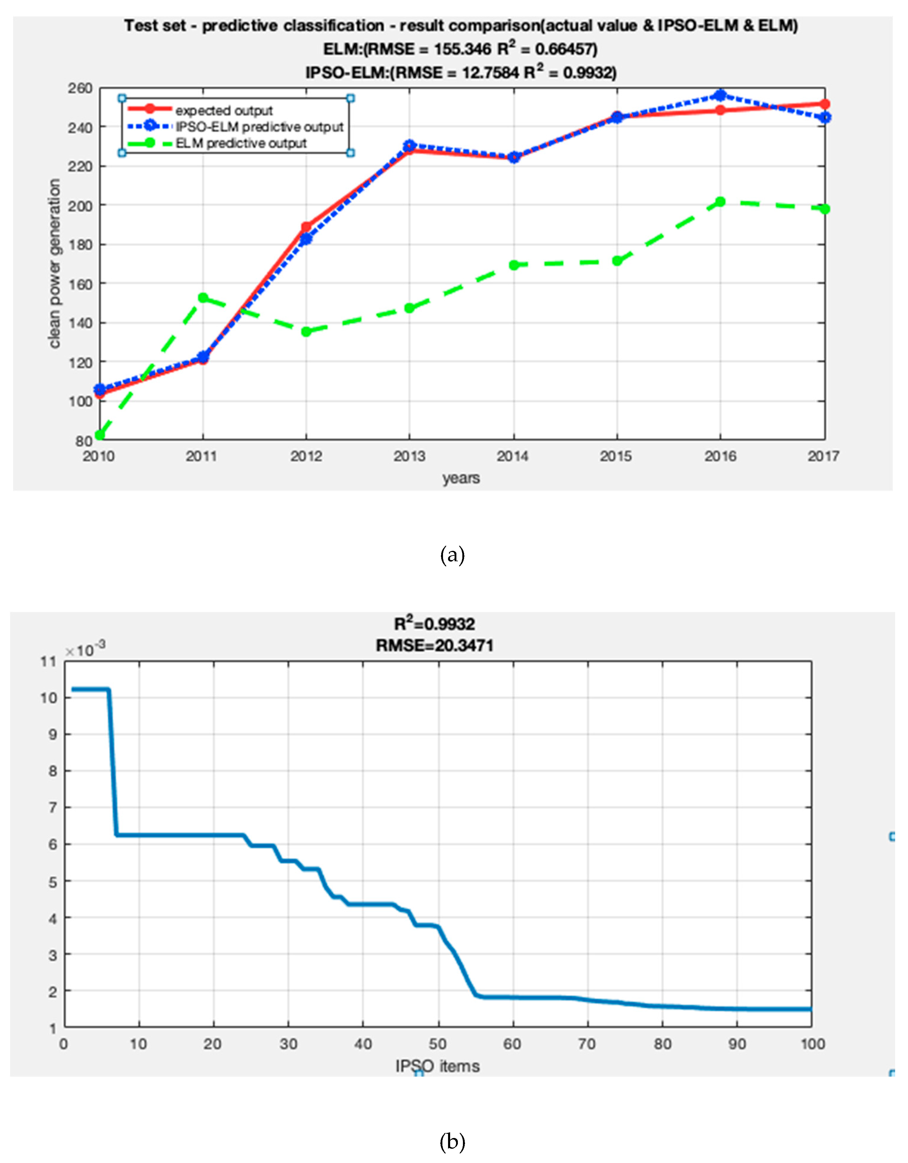
The Extreme learning machine optimized by Improved particle swarm optimization (IPSO-ELM) model is first applied in the field of energy mix prediction which has higher precision than the Extreme Learning Machine (ELM) predictive method; this method not only greatly improves the forecasting accuracy but also decreases the possibility of trapping a local minimum;

(3)

This paper pioneered a model of a correlational relationship between electric energy structure and number of electric vehicles under carbon constraint and calculated the maximum number of electric vehicles under the carbon emission reduction target.

2. Methodology

2.1. Improved Particle Swarm Optimization (IPSO)

Particle swarm optimization (PSO) is a robust optimization algorithm in which the optimal solution is found by iteration. It is initialized into a set of random particles with the speed and direction of each particle motion are determined according to the individual and group optimal information. The update process is as follows:

$$v_i^{k+1}=w{v}_i+c_{1}rand\left(p_{bi}^k-x_i^k\right)+c_{2}rand\left(g_b^k-x_i^k\right)$$

(1)

$$x_i^{k+1}=x_i^k+v_i^{k+1}$$

(2)

Here, the parameters c1 and c2 are accelerating factors. rand is a random number between [0,1]. Positive parameter w is the inertia weight. $v_i^k$ is the speed of the kth iteration of the i-th particle; $x_i^k$ is the position of the i-th particle at the kth iteration; $p{b}_i^k$ is the historical best of the k-th iteration of the i-th particle; $g_b^k$ is the best of group history at the kth iteration [25].

As can be seen from the above formula, the basic PSO algorithm introduces the speed update by introducing the group’s best and individual advantages. In the process of continuous iteration, it is closed to the best of the group. After the algorithm converges, all the particles are concentrated in the best of the group. However, the speed and position of all particles will not be updated after the algorithm converges. When the group’s best advantage is not the global optimal solution, the algorithm falls into local optimum called the algorithm “premature” [26]. In this paper, an improved particle update algorithm is developed based on the premature characteristics of the algorithm to avoid a premature algorithm. The specific steps are as follows:

Step 1

Initialize the decision vector P, P is a zero vector and the dimension is equal to the particle population of the particle group;

Step 2

Judge whether $\mathrm{D}{x}_i\le \epsilon$ is established, if it is established, then $\mathrm{P}\left(i\right)=\mathrm{P}\left(i\right)+1$; otherwise, $\mathrm{P}\left(i\right)=0$. Here, $\epsilon$ is the judgment accuracy, this paper set the $\epsilon$ for 10⁻⁵;

$$\mathrm{D}{x}_i={\left(g_b^k-x_i^k\right)}^T\left(g_b^k-x_i^k\right)$$

(3)

Step 3

If $\mathrm{P}\left(i\right)\ge 2$, it is determined that the i-th particle loses the optimization function and the particle position is reset to a random sequence.

Through this improved algorithm, when the particle loses the optimization function, the particle position is reset to a new sequence and the optimization function is restored, which can effectively avoid the algorithm premature.

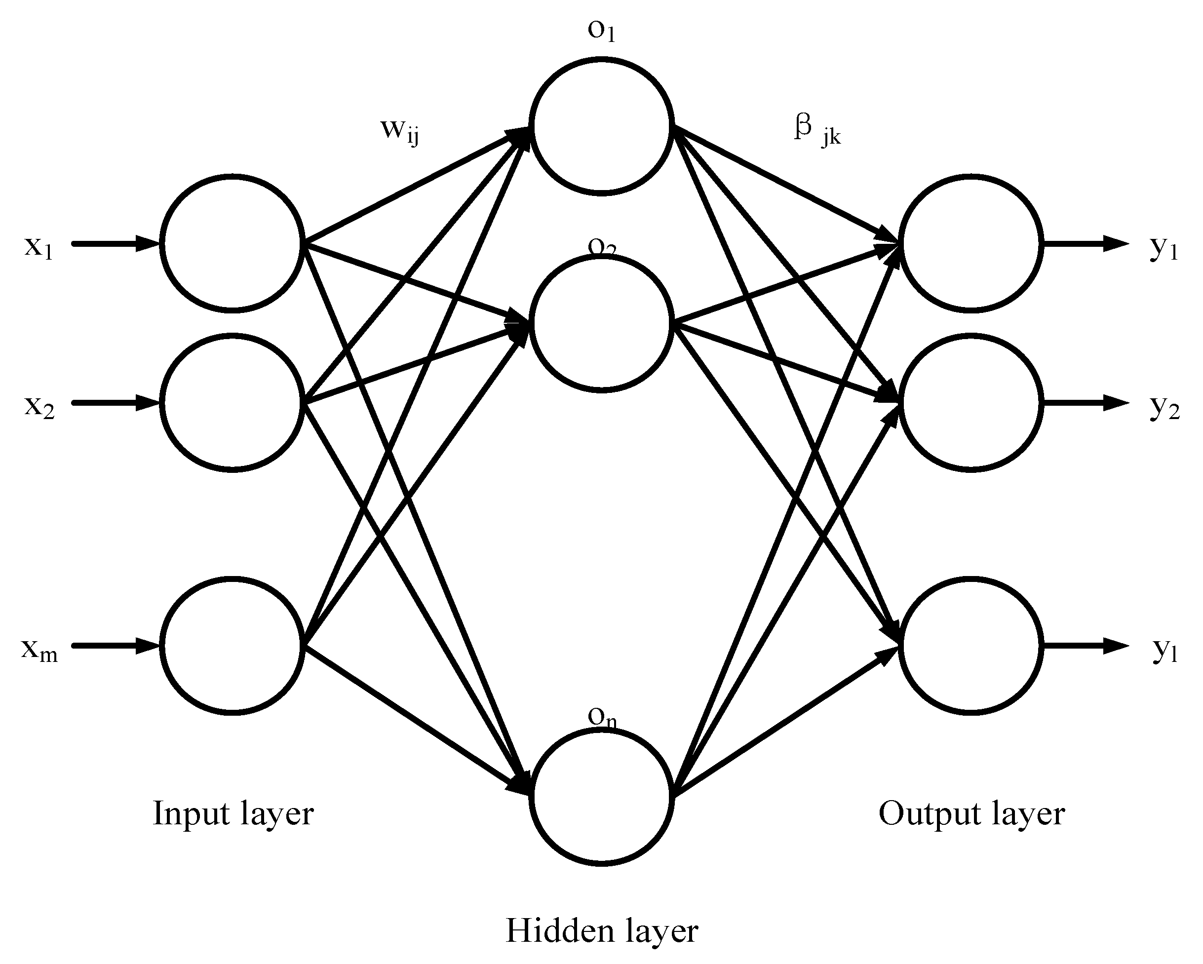
2.2. Extreme Learning Machine

As a new single hidden layer forward neural network learning algorithm, Extreme learning machine (ELM) is different from traditional neural network training learning in that the ELM hidden layer does not need iteration, input weight and hidden layer node offset are randomly selected and will be minimal, the minimum training error is the target and the hidden layer output weight is finally determined [27]. With the advantages of fast learning speed and good generalization performance compared with the traditional training method, ELM has attracted more attention from experts and scholars at home and abroad [28]. The neural network structure of ELM is shown in Figure 1. However, the ELM algorithm has the disadvantages of initial weight and excessive threshold. To solve the above problems, this paper proposes an improved particle swarm optimization (IPSO) method to optimize the initial parameters of the ELM model.

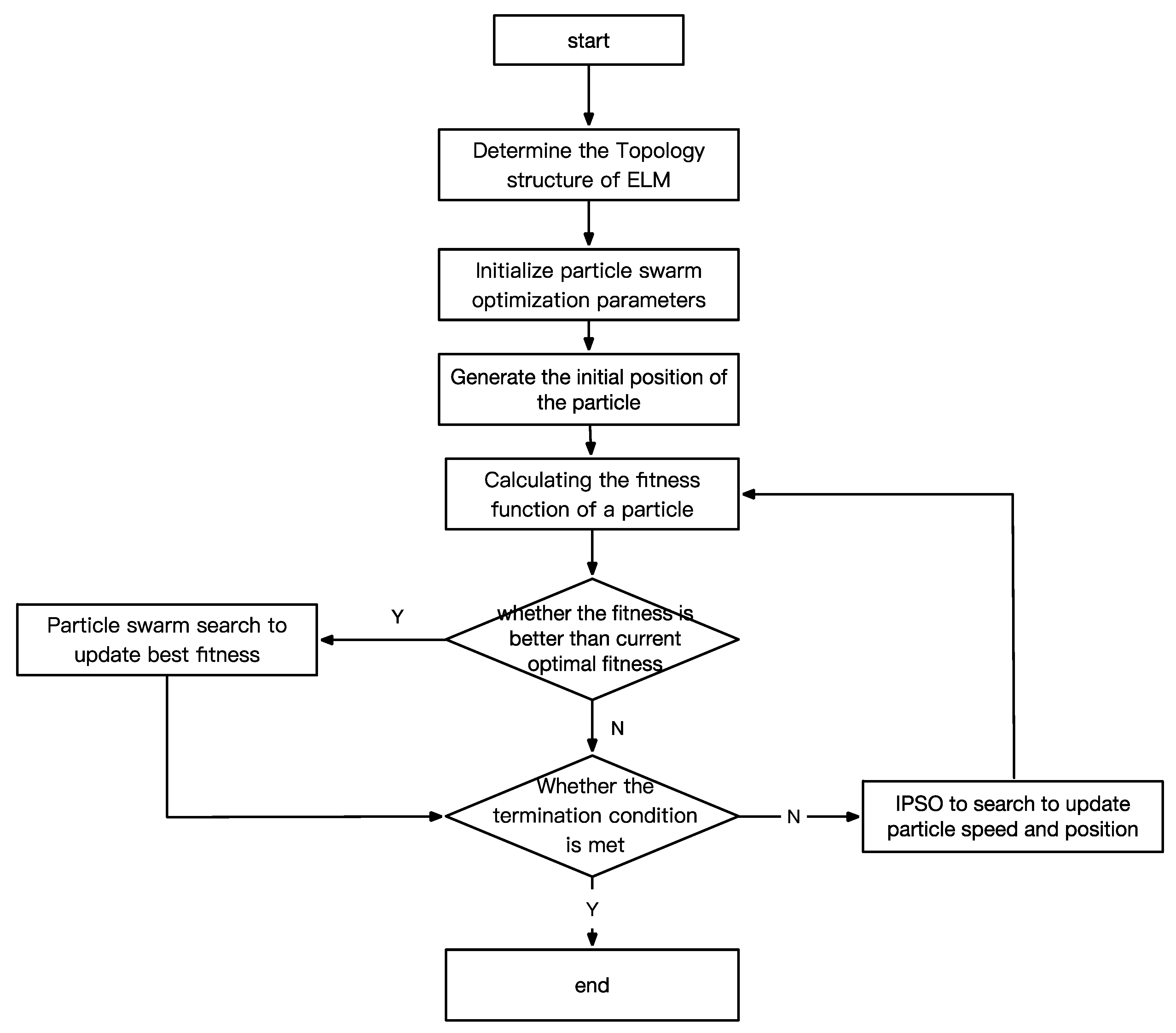
2.3. Extreme Learning Machine Optimized by Improved Particle Swarm Optimization

The input weight of the Extreme Learning Machine (ELM) and the threshold of the hidden layer are randomly given, if the input weight and the hidden layer threshold are 0, some hidden layer nodes may be invalid. Therefore, in the actual application process, a large number of hidden layer nodes need to be set to meet the accuracy requirements. Meanwhile, because the initial weight and threshold of the ELM are randomly generated, a big gap between each training and learning result may be generated. In view of the above problems, this paper proposed an improved particle swarm optimization extreme learning machine (IPSO-ELM) prediction algorithm. The specific steps are as Figure 2.

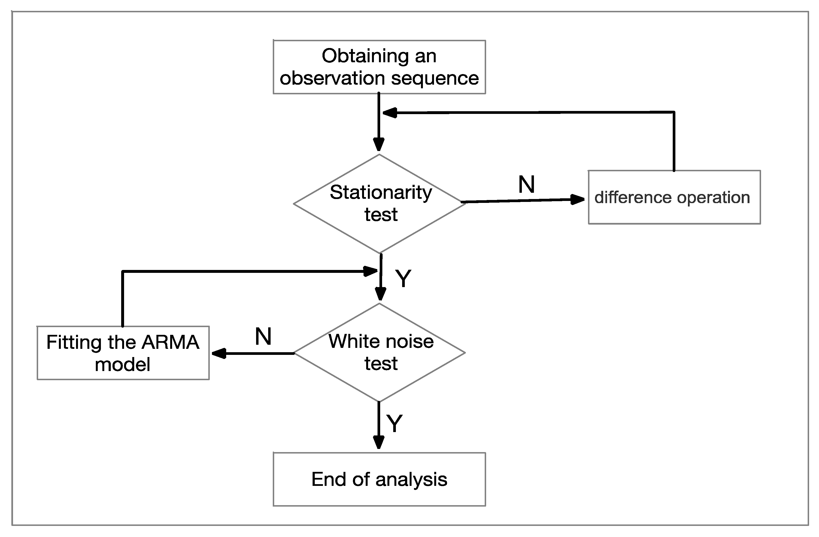
2.4. Autoregressive Integrated Moving Average Model (ARIMA)

Autoregressive Integrated Moving Average model (ARIMA) is a well-known time series method proposed by G.E.P.Box and G.M.jenkins in 1976 for the study of time series prediction and has been improved to derive many models with excellent precision [29]. The basic idea of ARIMA is to use a certain mathematical model to approximate the description and identify the time series of predicted objects to achieve the purpose of predicting the future value of the sequence based on historical observations. Specific modeling process is as Figure 3:

3. Electric Vehicles Ownership Calculation

3.1. Model of Correlational Relationship between Electric Energy Structure and Electric Vehicles Number under Carbon Constraint

Electric cars do not emit carbon emissions while driving. The power structure of the Beijing-Tianjin-Hebei region is mainly thermal power; in a sense, electric vehicles transfer the carbon emissions to thermal power generation [30]. Therefore, it is necessary to make further analysis about whether or not large-scale development of electric vehicles can achieve carbon emissions reduction targets and calculate the maximum number of electric vehicles that can achieve the carbon emission reduction target under the existing energy mix. The carbon emissions level of electric vehicles obviously depend on a power generation structure, since clean power produces fewer carbon emissions during its life cycle. In the case of the same number of vehicles, let the carbon emissions of electric vehicles equal those of traditional fuel vehicles, a relationship between regional energy structure and electric vehicle holdings is constructed.

(1)

Power consumption of electric vehicles ($Q_1$)

$$Q_1=\frac{q\times k\times S}{100\times {\eta }_2\times \left(1-\omega \right)}$$

(4)

$q$ is 100 km of electricity consumption per electric vehicle; k is electric vehicles holdings; ${\eta }_2$ is the charging efficiency of electric vehicles; $\omega$ is line loss rate during power transfer; S is the average annual travel distance of each electric car.

(2)

Carbon emissions from electric vehicles ($E_1$)

$$E_1=Q_1\times \left[E{F}_{clean}\times \frac{F_1}{F}+E{F}_{fire}\times \left(1-\frac{F_1}{F}\right)\right]$$

(5)

$E{F}_{clean}$ are the average carbon emissions factors of clean energy power generation; $E{F}_{fire}$ are carbon emissions factors of thermal power generation; $F_1$ is clean power generation in the Beijing-Tianjin-Hebei region (kW h); $F$ is the total power generation in the Beijing-Tianjin-Hebei region (kW h).

In the whole life cycle, clean energy produces fewer carbon emissions, so, in this paper, clean energy will not be classified using the average clean energy carbon emissions; in order to facilitate statistics and calculations, the energy prediction structures are only divided into clean energy generation and thermal power generation.

(3)

Carbon emissions from traditional fuel vehicles ($E_2$)

$$E_2={\displaystyle \sum }_{j=1}^{3}E{F}_j\times V_j\times S_j\times B\Rightarrow {\displaystyle \sum }_{j=1}^{3}E{F}_j\times M_j\times \frac{S}{100}\times S_j\times B$$

(6)

$E{F}_j$ are carbon emissions factors from three types of traditional fuel vehicles; $V_j$ is the amount of energy consumed per fuel vehicle per year; $M_j$ is the fuel consumption or natural gas volume of a traditional car of 100 km $B$ is traditional fuel cars holdings; $s_j$ is the proportion of three types of traditional fuel vehicles.

(4)

A relationship between energy mix structure and electric vehicles holdings

In order to study the maximum value of electric vehicles under the existing energy structure in the Beijing-Tianjin-Hebei region and ensures that the carbon emissions of electric vehicles are not higher than the traditional cars, a relationship between energy mix structure and electric vehicles holdings is established. In other words, when $E_1=E_2$, the value of k is the maximum value of the electric car in this case. The formula is calculated as follows:

$$E_1=E_2\Rightarrow Q_1\times \left[E{F}_{clean}\times \frac{F_1}{F}+E{F}_{fire}\times \left(1-\frac{F_1}{F}\right)\right]={\displaystyle \sum }_{j=1}^{3}E{F}_j\times V_j\times S_j\times B$$

$$\begin{gathered} \Rightarrow \frac{q\times k\times S}{{\eta }_2\times \left(1-\omega \right)\times 100}\left[E{F}_{clean}\times \frac{F_1}{F}+E{F}_{fire}\times \left(1-\frac{F_1}{F}\right)\right] \\ ={\displaystyle \sum }_{j=1}^{3}E{F}_j\times M_j\times \frac{S}{100}\times S_j\times B \end{gathered}$$

$$\Rightarrow k=\frac{\left({{\displaystyle \sum }}_{j=1}^{3}E{F}_j\times M_j\times S_j\times B\right)\times {\eta }_2\times \left(1-\omega \right)}{\left[E{F}_{clean}\times \frac{F_1}{F}+E{F}_{fire}\times \left(1-\frac{F_1}{F}\right)\right]\times q}$$

(7)

3.2. Energy Consumption Per 100 km (q)

The energy consumption of different types of cars is not the same. The energy consumption per 100 km of electric vehicles is exemplified by the power consumption of several mainstream electric vehicles on the market, the specific values are shown in

Table 1. Electricity consumption per 100 km of electric vehicles (kW h).

Car Manufacturer	BYD	SAIC Roewe	Chery	JAC	Geely	Changan
Model	E6	E50	eQ	iEV	Conti	EODO
Electricity consumption per 100 km	20	15	15	14	14	16
Average energy consumption per 100 km	15.7

[7];

3.3. Charging Efficiency of Electric Vehicles (${\eta }_2$)

In the process of the AC charging of electric vehicles, the charging efficiency of the electric vehicle will be determined by the on-board charger, the internal resistance of the battery and the battery temperature [31]. The higher the efficiency of the car charger, the lower the internal resistance of the battery and the more reasonable the battery temperature, the higher the charging efficiency of the electric vehicle will be [31]. To simplify the calculation, this paper uses the average charging efficiency. The specific charging efficiency is shown in

Table 2. Electric vehicle charging efficiency.

Manufacturer	BYD	SAIC Roewe	Chery	JAC	Geely	Changan
	E6	E50	eQ	iEV	Conti	EODO
SOH 100%	87.6%	87.5%	86.3%	86.9%	87.2%	87.6%
SOH 90%	86.5%	86.9%	85.5%	86.1%	87.1%	86.9%
Battery temperature 25 °C	88.1%	88%	87.1%	87.5%	88.4%	88.9%
Battery temperature 45 °C	83.1%	84.1%	83.4%	84.1%	84.1%	85.1%
Comprehensive efficiency	86.33%	86.63%	85.58%	86.15%	86.70%	87.13%
Average comprehensive efficiency	86.42

. (SOH: battery can store charge capacity).

3.4. Carbon Emission Coefficient for Different Energy Forms

The carbon emission coefficient refers to the amount of carbon emissions per unit of energy consumption. According to the assumptions of the United Nations Intergovernmental Panel on Climate Change (IPCC), the carbon emission coefficient of an energy source can be considered to be constant in the course of use [32]. From the perspective of the life cycle, there is also a small amount of carbon emissions from clean energy. This article draws on the research results of Dr. Ma Zhonghai [33]: The carbon emissions of the thermal power chain are 1303.0 g CO₂/kW h; according to a review by the World Nuclear Association of 23 relevant research reports since 1997, the carbon emissions of the hydroelectric chain are 26 g CO₂/kW h; the carbon emissions of the nuclear power chain are 29 g CO₂/kW h; the carbon emissions of wind power generation are 26 g/kW h (minimum 6 g/kW h, up to124 g/kW h). The carbon emissions of solar energy are 85 g/kW h [34].

Table 3. Carbon emission factors for various energy dioxides.

Fuel	Carbon Emissions (kg)
Gasoline (L) ($E{F}_1$)	2.36
Diesel (L) ($E{F}_2$)	2.63
Liquefied natural gas (kg) ($E{F}_3$)	1.964
Thermal power generation (kW h)$\left(E{F}_{fire}\right)$	1.303
Hydroelectric power (kW h)	0.026
Nuclear power generation (kW h)	0.029
Wind power generation (kW h)	0.026
Solar energy generation (kW h)	0.085
Clean power generation average (kW h)$\left(E{F}_{clean}\right)$	0.0415

Source: http://www.tanpaifang.com/tanjiliang/2014/0914/38053.html.

shows the carbon emission coefficient of different energy sources. (In the whole life cycle, clean energy produces fewer carbon emissions, so, in this paper, clean energy will not be classified using the average carbon emissions).

3.5. Clean Power Generation and Total Power Generation Forecasting

When calculating the electric vehicle equilibrium value k, it is necessary to predict the clean energy generation (F1) and total power generation (F) in the Beijing-Tianjin-Hebei region and analyze the ratio of the two to the Formula (7). In this paper, the Extreme learning machine optimized by Improved particle swarm optimization (IPSO-ELM) model is established with the influencing factors of gray correlation analysis used as an input, comparing the individual Extreme Learning Machine (ELM) models. Then the power generation is predicted.

3.5.1. Input Selection

In order to predict the regional power generation more accurately, the Grey Relational Analysis (GRA) method is introduced in this paper to select the input variables of the model. In other words, the influencing factors with a higher correlation with the regional power generation are selected as the input variables of the model.

The grey system theory was proposed by Professor Deng Julong and the Grey Relational Analysis (GRA) is an important part of the grey system theory. It is based on the degree of similarity of the sequence curves of things or factors to determine the degree of association. The more similar shape of two curves, the greater the degree of correlation will be, otherwise, the degree of association is smaller [35].

There are many influencing factors on power generation in theBeijing-Tianjin-Hebei region. Based on the relevant literature, the 10 characteristic sequences of power generation influencing factor changes are selected [36]. Clean power generation and total power generation in the Beijing-Tianjin-Hebei region are selected as parameter series; ${\mathrm{X}}_1$: average temperature; ${\mathrm{X}}_2$: sunshine hours; ${\mathrm{X}}_3$: precipitation; ${\mathrm{X}}_4$: average wind speed, ${\mathrm{X}}_5$: employment population, ${\mathrm{X}}_6$: GDP per capita, ${\mathrm{X}}_7$: consumer price index; ${\mathrm{X}}_8$: electricity consumption for domestic consumption; ${\mathrm{X}}_9$: coal price as a comparison series. The main purpose of GRA on the impact of power generation changes is to comprehensively and quantitatively evaluate the impact of these factors on power generation changes. Quantitative analysis of the GRA is carried out based on the current data of the Beijing-Tianjin-Hebei region from 1982 to 2017 (Appendix

Table A1. Verify historical data on the accuracy of the IPSO-ELM method.

Year	X1	X2	X3	X4	X5	X6	X7	X8	X9	Y1	Y2
1982	12.8	2825.1	544.4	2.6	68.996	3326.4	101.8	12.345	25.730	0.583	29.165
1983	13	2844.3	489.9	2.4	70.521	3672.9	100.5	12.645	26.380	0.625	31.275
1984	11.9	2767.6	488.8	2.4	71.724	4378.5	102.2	13.354	27.210	0.671	33.553
1985	11.5	2511.9	721	2.2	72.821	5405.4	117.6	14.139	31.960	0.731	36.552
1986	12.1	2804.1	665.3	2.3	73.817	6066.9	106.8	14.603	34.760	0.800	40.006
1987	12.3	2631.9	683.9	2.4	75.048	7005.6	108.6	15.333	47.290	0.885	44.260
1988	12.7	2558.1	673.3	2.4	76.233	8605.8	120.4	16.137	51.230	0.970	48.523
1989	13.2	2626.2	442.2	1.9	76.933	9569.7	117.2	16.497	56.340	1.041	52.047
1990	12.7	2325	697.3	1.9	78.121	10,357.2	105.4	17.005	61.670	1.106	55.287
1991	12.5	2536.6	747.9	2.1	79.294	11,925.9	111.9	18.203	70.930	1.206	60.298
1992	12.8	2712.5	541.5	2.2	80.217	14,559.3	109.9	20.376	85.130	1.342	67.097
1993	13	2669.8	506.7	2.6	80.901	18,887.4	119.0	22.369	113.650	1.492	74.609
1994	13.7	2470.5	813.2	2.5	81.650	25,477.2	124.9	24.619	126.830	1.648	82.414
1995	13.3	2519.1	572.5	2.6	82.435	31,789.8	117.3	26.336	140.440	1.784	89.205
1996	12.7	2418.7	700.9	2.6	83.216	36,829.8	111.6	28.567	159.410	1.916	95.800
1997	13.1	2596.5	430.9	2.5	83.975	40,446.0	105.3	29.087	166.600	2.076	101.874
1998	13.1	2420.7	731.7	2.3	84.746	42,814.8	102.4	29.678	160.200	1.705	99.701
1999	13.1	2594	266.9	2.4	85.442	45,101.7	100.6	31.484	143.980	1.156	109.411
2000	12.8	2667.2	371.1	2.5	87.712	49,067.0	103.5	33.999	140.190	1.361	120.111
2001	12.9	2611.7	338.9	2.4	87.754	54,390.0	103.1	37.056	150.590	0.668	125.234
2002	13.2	2588.4	370.4	2.3	88.147	61,187.0	98.2	40.242	167.810	0.974	142.507
2003	12.9	2260.2	444.9	2.5	88.565	70,687.0	100.2	51.638	173.540	0.969	160.057
2004	13.5	2515.4	483.5	2.4	130.242	84,161.0	101.0	61.202	210.000	1.027	179.921
2005	13.2	2576.1	410.7	2.4	140.281	96,009.0	101.5	70.518	240.000	1.338	192.104
2006	13.4	2192.7	318	2.2	154.877	107,360.0	100.9	76.232	270.000	2.992	203.509
2007	14	2351.1	483.9	2.2	170.558	127,728.0	102.4	86.248	304.810	1.827	226.759
2008	13.4	2391.4	626.3	2.2	191.767	146,133.0	105.1	96.029	418.550	12.484	215.336
2009	13.3	2511.8	480.6	2.2	226.492	154,095.0	98.5	108.293	394.350	6.299	240.088
2010	12.6	2382.9	522.5	2.3	257.692	175,518.0	102.4	117.936	453.310	10.352	285.120
2011	13.4	2485.7	720.6	2.2	272.462	200,840.0	105.6	126.941	498.430	12.130	321.102
2012	12.9	2450.2	733.2	2.2	306.040	217,232.0	103.3	135.965	500.230	18.879	330.043
2013	12.8	2371.1	578.9	2.1	342.108	233,662.0	103.3	141.563	520.260	22.770	340.354
2014	14.1	2344.1	461.5	2.1	377.331	245,210.0	101.6	152.770	529.250	22.398	348.939
2015	13.7	2420.2	458.6	2.1	405.265	254,712.0	101.8	153.270	548.930	24.499	354.200
2016	15.2	2530.3	432.3	2	428.031	276,313.0	101.4	159.678	610.250	24.798	367.200
2017	16.1	2638.4	467.2	2.1	426.198	288,065.1	101.3	158.843	600.084	25.156	371.741

for detailed data). The results of the correlation analysis of various factors are shown in

Table 4. Correlation analysis of 10 influencing factors of clean power generation.

Influencing Factors	Score	Influencing Factors	Score
average temperature	−0.363	GDP per capita	0.910
sunshine hours	0.431	consumer price index	0.834
precipitation	0.088	electricity consumption for domestic consumption	0.888
average wind speed	0.436	coal price	0.879
employment population	0.959

and

Table 5. Correlation analysis of 10 influencing factors of total power generation.

Influencing Factors	Score	Influencing Factors	Score
average temperature	−0.359	GDP per capita	0.991
sunshine hours	0.413	consumer price index	0.813
precipitation	0.102	electricity consumption for domestic consumption	0.986
average wind speed	0.374	coal price	0.991
employment population	0.944

.

From Table 1 and Table 2, we select the factors with a higher correlation and correlation coefficient higher than 0.85 as the main influencing factors affecting clean energy generation and total power generation. Consistently, the main factors affecting clean energy generation and total power generation are the following five factors: employment population, GDP per capita, consumer price index, electricity consumption for domestic consumption and coal price.

3.5.2. Model Error Analysis

In the MATLAB 2016a environment, Extreme learning machine optimized by Improved particle swarm optimization (IPSO-ELM) and Extreme Learning Machine (ELM) are applied to predict the power generation of clean power and total power generation. The historical data from 1982 to 2010 was used as training data and the data from 2011–2017 was used as test data (Appendix A for detailed data). The 5 factors affecting clean and total power generation (GDP per capita, coal price, electricity consumption for domestic consumption, installed capacity, employment population) selected by GRA are used as inputs. The clean power generation and total power generation in Beijing-Tianjin-Hebei region as outputs. In the process of Extreme learning machine optimized by Improved particle swarm optimization (IPSO-ELM), connection weight and threshold, the relevant parameters are set as shown in

Table 6. IPSO-ELM parameter settings.

Parameter	Set Quantity
the max-generation	40
the size of population	40
The maximum number of iterations	300

. The results are shown in Figure 4a,b and Figure 5a,b.

As illustrated in Figure 4a and Figure 5a, by comparing the predicted value with the true value, we can conclude that the predicted value of the IPSO-ELM model is best fitted to the actual value in the power generation forecast compared to the ELM model that has large deviations at individual points. Obviously, IPSO-ELM is suitable for predicting the amount of power generated, which can significantly improve the prediction accuracy.

The results and analysis of the power generation forecast are shown in Figure 4 and Figure 5. The values of RMSE and R2 are shown in

Table 7. Error analysis of comparative models.

Parameter	Index	ELM	IPSO-ELM
Forecast of clean power generation	R²	66.46%	99.32%
	RMSE	155.346	12.76
Forecast of total power generation	R²	91.73%	99.29%
	RMSE	241.20	62.48

. With a reasonable selection of factors, compared with the ELM model, the RMSE of IPSO-ELM is smaller, at 3.38 and 56.2, while R2 is larger at higher than 99%, indicates that the prediction accuracy of IPSO-ELM model is higher than that of the ELM model and more suitable for the prediction of the power generation in the Beijing-Tianjin-Hebei region.

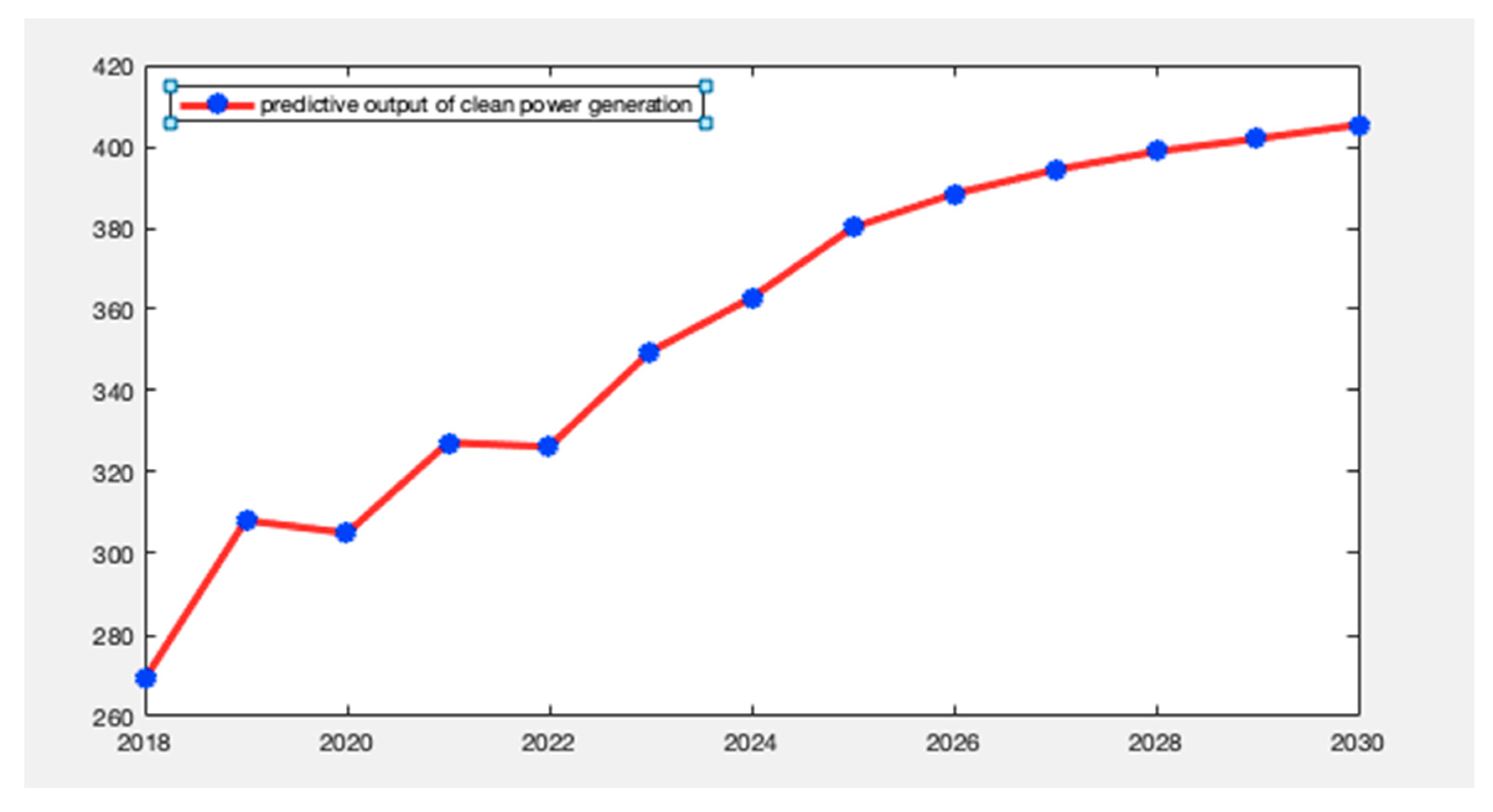
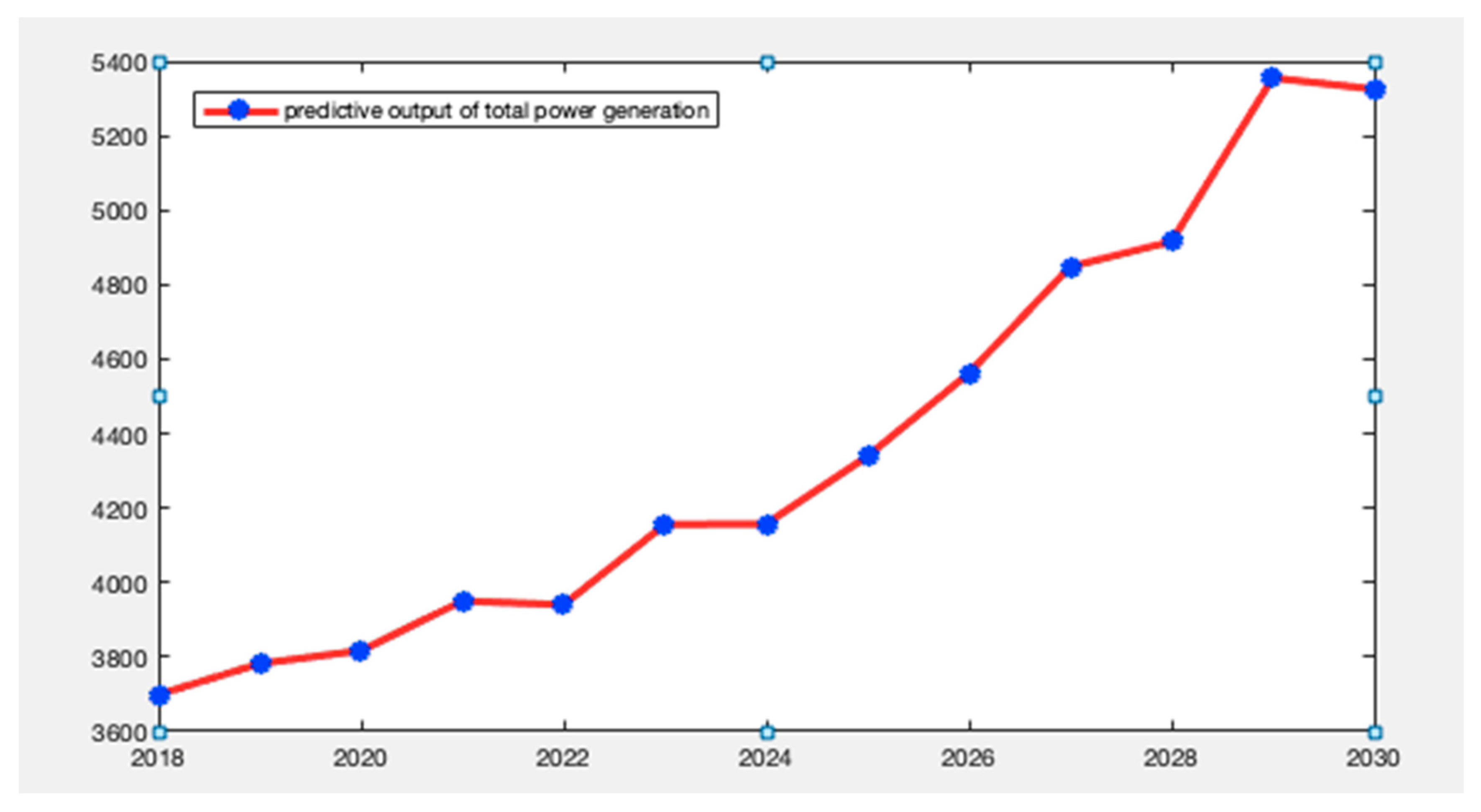
3.5.3. Forecast of Power Generation in the Beijing-Tianjin-Hebei Region from 2018 to 2030

In this paper, the values of 5 influencing factors selected by GRA in 2018–2030 are predicted as input data by the method of Autoregressive Integrated Moving Average (ARIMA), which was proposed by Box and Jenkins as a method for predicting the stability of time series (Appendix

Table A2. Forecast values of five influencing factors in 2018–2030 through the ARIMA method.

Year	X5	X6	X7	X8	X9
2018	449.670	294,109.7	101.0	169.847	634.037
2019	469.534	313,876.4	99.0	168.116	663.942
2020	485.237	317,094.0	101.1	177.035	676.726
2021	496.431	335,087.3	100.4	178.350	675.639
2022	502.985	339,166.9	98.3	183.811	677.093
2023	504.992	358,870.7	100.5	188.778	695.090
2024	502.769	366,171.5	99.3	190.563	727.932
2025	496.835	388,416.9	97.7	199.067	759.835
2026	487.890	398,163.0	99.8	197.606	775.905
2027	476.781	421,017.7	98.1	208.925	776.274
2028	464.459	430,701.0	97.2	205.204	775.972
2029	451.933	451,843.4	99.0	218.130	790.668
2030	440.225	459,846.2	97.1	213.525	821.796

for predicted data).

The IPSO-ELM model is used to predict clean power generation and total power generation in this paper and the clean power generation and total power generation forecasting are shown in the Figure 6 and Figure 7.

It is clear that the clean energy power generation and total power generation in the Beijing-Tianjin-Hebei region have shown an expected upward trend in 2018–2030.

Table 8. Forecast of clean power generation and total power generation in the Beijing-Tianjin-Hebei region in 2019, 2020 and 2030 (billion kW h).

Year	Clean Power Generation	Total Power Generation
2020	30.504	381.738
2030	40.535	532.525

shows the forecast data for typical years. (See Appendix

Table A3. The predicted value of clean energy generation (Y1) and total power generation (Y2) in 2018–2030 through the IPSO-ELM method.

Year	Y1	Y2	Year	Y1	Y2
2018	26.913	369.919	2024	36.285	415.745
2019	30.815	378.226	2025	38.011	433.933
2020	30.504	381.739	2026	38.840	456.195
2021	32.727	395.024	2027	39.430	484.839
2022	32.625	394.073	2028	39.880	491.566
2023	34.962	415.616	2029	40.195	535.526
			2030	40.536	532.525

for specific data).

4. Results

The following conditions are assumed:

(a)

The comprehensive line loss rate (${\eta }_2$) used to calculate the carbon emissions is 6.17% [37];

(b)

The energy consumption per 100 km of traditional fuel vehicles is calculated based on the average fuel consumption on the market. This paper assumes that fuel vehicles consume 8 L per 100 km ($M_1$, $M_2$) and natural gas-fueled vehicles consume 5.3 kg of natural gas per 100 km ($M_3$) by data statistics;

(c)

In traditional fuel cars, the ratio of gasoline vehicles ($S_j$), diesel vehicles and natural gas vehicles are 12:5:3 [38].

The method of Autoregressive Integrated Moving Average (ARIMA) is used to predict the number of traditional fuel cars from 2018–2030 with the historical statistics from 2000–2017. Data can be queried from the National Bureau of Statistics. (For historical data on the number of traditional cars, see Appendix

Table A4. Number of traditional fuel vehicles in 2000–2017.

Year	2000	2001	2002	2003	2004	2005	2006	2007	2008
the number of traditional fuel cars (million)	2.561	2.791	3.180	3.725	4.217	4.756	5.477	6.399	7.389
year	2009	2010	2011	2012	2013	2014	2015	2016	2017
the number of traditional fuel cars (million)	8.939	11.008	12.685	14.432	15.950	17.351	18.825	20.670	22.380

).

Table 9. The number of traditional fuel cars predicted in 2018–2030.

Year	2018	2019	2020	2021	2022	2023	2024
traditional fuel cars(million)	23.99	24.31	25.56	26.02	26.9	27.35	28.09
Year	2025	2026	2027	2028	2029	2030
traditional fuel cars(million)	28.8	29.08	29.87	30.32	33.98	36.09

shows the number of traditional fuel cars predicted in 2018–2030.

From the 3.4, Table 5 shows that the carbon emissions factors of gasoline, diesel and liquefied natural gas are 2.36, 2.63 and 1.964. At this time, according to Formula (7), under carbon emission reduction constraints, a relationship between regional energy structure and electric vehicles holdings can be expressed as:

$$\begin{array}{l}k=\Rightarrow k=\frac{\left({{\displaystyle \sum }}_{j=1}^{3}E{F}_j\times M_j\times S_j\times B\right)\times {\eta }_2\times \left(1-\omega \right)}{\left[E{F}_{clean}\times \frac{F_1}{F}+E{F}_{fire}\times \left(1-\frac{F_1}{F}\right)\right]\times q}\\ =\frac{\left(2.36\times 8\times 60\%+2.63\times 8\times 25\%+1.964\times 5.3\times 15\%\right)\times 86.42\%\times \left(1-6.17\%\right)\times \mathrm{B}}{\left[0.0415\times \frac{F_1}{F}+1.303\times \left(1-\frac{F_1}{F}\right)\right]\times 15.7}\Rightarrow \end{array}$$

$$k=\frac{206.22\times B}{\left[0.0415\times \frac{F_1}{F}+1.303\times \left(1-\frac{F_1}{F}\right)\right]}$$

(8)

Based on the above relationship mode (Equation (8)) and regional energy structure predictions (Table 8). The maximum electric vehicles holdings in the Beijing-Tianjin-Hebei region under carbon constraints in 2020, 2030 and regional clean energy generation, according to the national electric vehicle quantity plan, are shown in

Table 10. Electric vehicles holdings in 2020 and 2030 in Beijing-Tianjin-Hebei region.

Year	2020	2030
Clean power generation (billion kW h)	30.041	40.535
Total power generation (billion kW h)	381.739	532.525
The maximum quantity of electric vehicles under the carbon emission reduction target by eliminating clean energy (million units)	18.37	26.86
the number of traditional fuel cars (million units)	23.06	32.57
the ratio of the number of electric vehicles to the number of traditional cars	0.75	0.78
the proportion of clean energy generation to achieve a complete replacement of traditional fuel vehicles for electric vehicles	0.314	0.323

. The following conclusions can be drawn:

(a)

The maximum quantity of electric vehicles under the carbon emission reduction target by eliminating clean energy is 0.4385 million and 0.6167 million with the ratio of the number of electric vehicles to the number of traditional cars is 0.75 and 0.78, which shows that under the existing energy mix structure, electric vehicles cannot completely replace traditional vehicles to ensure carbon emission reduction.

(b)

In order to achieve a complete replacement of traditional fuel vehicles for electric vehicles, the minimum proportion of clean energy generation is 0.314 and 0.323 in 2020 and 2030, respectively, which shows it is necessary to introduce a large amount of clean energy, such as inter-regional power trading. Only in this way, with the carbon emission reduction target, can electric cars completely replace traditional fuel cars.

5. Conclusions

Due to the influence of the power structure and clean energy utilization rate in China, the promotion of electric vehicles based on the purpose of environmental protection and carbon emission reduction should be kept to a restrained scale and programmed step by step. A relationship between regional energy mix structure and electric vehicles holdings model is established on the basis of calculating and analyzing carbon emissions of different types of energy consumption. The Extreme learning machine optimized by Improved particle swarm optimization (IPSO-ELM) helps to forecast the growth trend of clean power generation and total power generation; the contrast test shows that IPSO-ELM makes the prediction results more accurate. The conclusions are as follows:

(a)

The main factors affecting regional clean power generation and total generation include: employment population, installed capacity, regional per capita GDP, total domestic consumption of electricity and coal price;

(b)

In consideration of the life cycle of environmental emissions of different energy sources, whether the large-scale development of electric vehicles can achieve environmental protection and carbon emission reduction depends on the regional electricity structure and clean energy utilization;

(c)

With the growth speed of clean power generation in the Beijing-Tianjin-Hebei region predicted by the IPSO-ELM method, when the number of officially planned electric vehicles is reached in 2020 and 2030, the carbon emissions of the large-scale adoption of electric vehicles are not lower than those of traditional fuel vehicles. That is to say, according to the prediction result of the generation of clean energy, the goal of carbon emission reduction by the large-scale development of electric vehicles cannot be achieved. It is necessary for local power grids to increase the proportion of clean energy consumption and the amount of clean power trading across provinces.

References

1. Hua, H.; Yong, C.; Qi, L. Bi-level multi-objective optimization dispatch of electric vehicles and new energy sources with the priority of satisfaction and cleanliness. Electr. Meas. Instrum. 2018, 55, 59–66, 79. [Google Scholar]
2. Chen, Z.; Liu, Q.; Xiao, X.; Liu, N.; Yan, X. Integrated Mode and Key Issues of Renewable Energy Sources and Electric Vehicles’ Charging and Discharging Facilities in Microgrid. Trans. China Electrotech. Soc. 2013, 28, 1–14. [Google Scholar] [CrossRef]
3. Baptista, P.; Ribau, J.; Bravo, J.; Silva, C.; Adcock, P.; Kells, A. Fuel cell hybrid taxi life cycle analysis. Energy Policy 2011, 39, 4683–4691. [Google Scholar]
4. Deluchi, M.A. Addendum to emissions of greenhouse gases from the use of transportation fuels and electricity. Effect of 1992 revision of global warming potential (GWP) by the Intergovernmental Panel on Climate Change (IPCC). In Office of Scientific & Technical Information Technical Reports; Argonne National Lab.: Argonne, IL, USA, 1992. [Google Scholar]
5. Hacknhy, J.; Neufville, R.D. Life cycle model of alternative fuel vehicles: Emissions, energy and cost tradeoffs. Transp. Res. Part A: Policy Pr. 2001, 35, 243–266. [Google Scholar]
6. Ou, X.M.; Zhang, X.L.; Qin, Y.N.; Qi, T.Y. Life cycle analysis of electric vehicle charged by advanced technologies coal-power in future China. J. China Coal Soc. 2010, 35, 169–172. [Google Scholar]
7. Shi, X.Q.; Li, X.N.; Yang, J.X. Research on Carbon Reduction Potential of Electric Vehicles for Low-Carbon Transportation and Its Influencing Factors. Chin. J. Environ. Sci. 2013, 34, 385–394. [Google Scholar]
8. Tang, B.J.; Ma, Y.; Wei, Y.M. Analysis of Energy Conservation and Emission Reduction of New Energy Vehicles in Beijing during the “13th Five-Year Plan”. J. Beijing Inst. Technol. (Soc. Sci. Ed.) 2016, 18, 13–17. [Google Scholar] [CrossRef]
9. Mishina, Y.; Muromachi, Y. Are potential reductions in CO2 emissions via hybrid electric vehicles actualized in real traffic? Case Jpn. Transp. Res. Part D 2017, 50, 372–384. [Google Scholar] [CrossRef]
10. Mills, G.; Macgill, I. Assessing greenhouse gas emissions from electric vehicle operation in Australia using temporal vehicle charging and electricity emission characteristics. Int. J. Sustain. Transp. 2017, 11, 20–30. [Google Scholar] [CrossRef]
11. Wang, G. Study on the Current Situation and Development Trend of Electric Vehicle Technology. Adv. Power Syst. Hydroelectr. Eng. 2017, 33, 97–100. [Google Scholar]
12. Doucette, R.T.; McCulloch, M.D. Modeling the prospects of plug-in hybrid electric vehicles to reduce CO2 emissions. Appl. Energy 2011, 88, 2315–2323. [Google Scholar] [CrossRef]
13. Patrick, J.; Sonja, B.; Wolf, F. Assessing CO2 emissions of electric vehicles in Germany in 2030. Transp. Res. Part A 2015, 78, 68–83. [Google Scholar]
14. Thiel, C.; Perujo, A.; Mercier, A. Cost and CO2 aspects of future vehicle options in Europe under new energy policy scenarios. Energy Policy 2010, 38, 7142–7151. [Google Scholar] [CrossRef]
15. Nanaki, E.A.; Koroneos, C.J. Comparative economic and environmental analysis of conventional, hybrid and electric vehicles—the case study of Greece. J. Clean. Prod. 2013, 53, 261–266. [Google Scholar] [CrossRef]
16. Huang, Y.; Ji, J.; Ma, X. Greenhouse gas emissions reduction from battery electric automobile: A study based on EIO-LCA model. China Environ. Sci. 2012, 32, 947–953. [Google Scholar]
17. Van den Broek, M.; Faaij, A.; Turkenburg, W. Planning for an electricity sector with carbon capture and Storage: Case of the Netherlands. Int. J. Greenh. Gas Control 2008, 2, 105–129. [Google Scholar] [CrossRef]
18. Brady, J.; O’Mahony, M. The potential impacts of electric vehicles on climate change and urban air quality. Transp. Res. Part D 2011, 16, 188–193. [Google Scholar] [CrossRef]
19. Yu, C.; Tan, Z.F.; Jiang, H.Y. Grey Incidence Analysis and Forecast on Energy Consumption and Economy Growth of China. J. Electr. Power 2007, 22, 424–427, 431. [Google Scholar] [CrossRef]
20. Liu, R.Y.; Zhang, J.; Huang, Q.; Lei, B.D. Energy Forecast Model Based on Combination of GM(1,1) and Neural Network. In Proceedings of the 2009 International Conference on Computational Intelligence and Software Engineering, Wuhan, China, 11–13 December 2009. [Google Scholar]
21. Yan, X.; Mu, L. Research on GM(1,1) Energy Prediction Model Based on Genetic Algorithm Optimization. China Manag. Inf. 2009, 12, 95–97. [Google Scholar]
22. Gorucu, F.B.; Geris, P.U.; Gumrah, F. Artificial neural network modeling for forecasting gas consumption. Energy Sources 2004, 26, 299–307. [Google Scholar] [CrossRef]
23. Szoplik, J. Forecasting of natural gas consumption with artificial neural networks. Energy 2015, 85, 208–220. [Google Scholar] [CrossRef]
24. Junchen, L.; Xiucheng, D.; Jian, G. Dynamical modeling of natural gas consumption in China. Nat. Gas Ind. 2010, 30, 127–129. [Google Scholar] [CrossRef]
25. Anand, A.; Suganthi, L. Hybrid GA-PSO Optimization of Artificial Neural Network for Forecasting Electricity Demand. Energies 2018, 11, 728. [Google Scholar] [CrossRef]
26. Qin, H.S.; Wei, D.Y.; Li, J.H.; Zhang, L.; Feng, Y.Q. A Particle Swarm Optimization with Variety Factor. Appl. Mech. Mater. 2013, 239, 1291–1297. [Google Scholar] [CrossRef]
27. Huang, G.B.; Zhu, Q.Y.; Siew, C.K. Extreme learning machine: A new learning scheme of feedforward neural networks. In Proceedings of the IEEE International Joint Conference on Neural Networks (IJCNN), Budapest, Hungary, 25–29 July 2004. [Google Scholar]
28. Luo, J.-X.; Luo, D.; Hu, Y.-M. A new online extreme learning machine with varying weights and decision level fusion for fault detection. Control Decis. 2018, 33, 1033–1040. [Google Scholar]
29. Wang, Y.W.; Shen, Z.Z.; Yan, B.H.; Yang, Y. Application of ARIMA and hybrid ARIMA-GRNN models in forecasting AIDS incidence in China. Chin. J. Dis. Control Prev. 2018, 22, 1287–1290. [Google Scholar] [CrossRef]
30. Ensslen, A.; Schücking, M.; Jochem, P.; Steffens, H.; Fichtner, W.; Wollersheim, O.; Stella, K. Empirical carbon dioxide emissions of electric vehicles in a French-German commuter fleet test. J. Clean. Prod. 2016, 142, 263–278. [Google Scholar] [CrossRef]
31. Vaka, R.; Keshri, R.K. Review on Contactless Power Transfer for Electric Vehicle Charging. Energies 2017, 10, 636. [Google Scholar] [CrossRef]
32. Yu, S.; Wei, Y.M.; Guo, H.; Ding, L. Carbon emission coefficient measurement of the coal-to-power energy chain in China. Appl. Energy 2014, 114, 290–300. [Google Scholar] [CrossRef]
33. Pan, Z.; Ma, Z.; Li, X.; Wu, T.; Xiu, B. Comparative study of impacts of coal chain and nuclear power chain in china on health, environment and climate. Radiat. Prot. 2001, 21, 129–145. [Google Scholar]
34. BJX.com.cn. Available online: http://news.bjx.com.cn/html/20171225/869765.shtml (accessed on 25 December 2017).
35. Yang, N.; Li, H.; Yuan, J.; Li, S.; Wang, X. Medium-and Long-term Load Forecasting Method Considering Grey Correlation Degree Analysis. Proc. CSU-EPSA 2018, 30, 108–114. [Google Scholar]
36. Guo, W.Q.; Shi, S.; Zhang, X.; Li, K.K.; She, J.L.; Gao, W.Q. Short-term power generation prediction based on BPneural network optimized by genetic algorithm. J. Shaanxi Univ. Sci. Technol. (Nat. Sci. Ed.) 2017, 35, 159–163, 178. [Google Scholar]
37. Min, T.; Xinghua, W.; Qing, L. Application of Support Vector Machine Based on Particle Swarm Optimization in Low Voltage Line Loss Prediction. In Proceedings of the Joint International Mechanical, Electronic and Information Technology Conference (JIMET), Chongqing, China, 18–20 December 2015. [Google Scholar]
38. Chinabaogao. Available online: http://zhengce.chinabaogao.com/nengyuan/2017/11203021512017.html (accessed on 15 February 2017).
Figure 1. Extreme learning machine (ELM) model structure.
Sustainability 11 02928 g001
Figure 2. Improved particle swarm optimization extreme learning machine (IPSO-ELM) algorithm process.
Sustainability 11 02928 g002
Figure 3. Autoregressive Integrated Moving Average model (ARIMA) model modeling process.
Sustainability 11 02928 g003
Figure 4. (a) Forecast of clean power generation in Beijing-Tianjin-Hebei region; (b) RMSE rate of clean power generation in Beijing-Tianjin-Hebei region.
Sustainability 11 02928 g004
Figure 5. (a) Forecast of total power generation in Beijing-Tianjin-Hebei region; (b) RMSE rate of total power generation in Beijing-Tianjin-Hebei region.
Sustainability 11 02928 g005
Figure 6. Forecast of clean power generation in 2018–2030.
Sustainability 11 02928 g006
Figure 7. Forecast of total power generation in 2018–2030.
Sustainability 11 02928 g007