Modeling the Impact of Climate Change and Land Use Change Scenarios on Soil Erosion at the Minab Dam Watershed

Abstract

Climate and land use change can influence susceptibility to erosion and consequently land degradation. The aim of this study was to investigate in the baseline and a future period, the land use and climate change effects on soil erosion at an important dam watershed occupying a strategic position on the narrow Strait of Hormuz. The future climate change at the study area was inferred using statistical downscaling and validated by the Canadian earth system model (CanESM2). The future land use change was also simulated using the Markov chain and artificial neural network, and the Revised Universal Soil Loss Equation was adopted to estimate soil loss under climate and land use change scenarios. Results show that rainfall erosivity (R factor) will increase under all Representative Concentration Pathway (RCP) scenarios. The highest amount of R was 40.6 MJ mm ha⁻¹ h⁻¹y⁻¹ in 2030 under RPC 2.6. Future land use/land cover showed rangelands turning into agricultural lands, vegetation cover degradation and an increased soil cover among others. The change of C and R factors represented most of the increase of soil erosion and sediment production in the study area during the future period. The highest erosion during the future period was predicted to reach 14.5 t ha⁻¹ y⁻¹, which will generate 5.52 t ha⁻¹ y⁻¹ sediment. The difference between estimated and observed sediment was 1.42 t ha⁻¹ year⁻¹ at the baseline period. Among the soil erosion factors, soil cover (C factor) is the one that watershed managers could influence most in order to reduce soil loss and alleviate the negative effects of climate change.

1. Introduction

Climate change and land use change relate to one another. Land use change is a driver of climate change, and a changing climate can lead to land cover changes [1]. For example, farmers may convert to crops of higher efficiency due to conditions of climate change and adjust land use to the new climate [2]. The increase of temperature leads to drought and consequently to the degradation of vegetation cover since it is dependent on water. Also, land use change affects climate due to the global levels of greenhouse gases [3].

Soil erosion has become a major challenge for environment and natural resources in the present century. Nowadays, the arable land annual soil loss in the world is 75 billion tons [4] and is more than 0.5 billion tons for Iran alone [5]. The cost of soil erosion was calculated to be approximately US $10.8 billion due to the loss of soil fertility and reservoir sedimentation (estimated by average price of the fertilizers and decrease of dam lifetime) [6].

All of these factors have led experts to stress the growing trend of soil erosion in Iran and emphasize the need to pay particular attention to water and soil conservation in order to achieve sustainable development. Researchers have been considering the importance of paying attention to traditional methods of water and soil conservation, optimal utilization of resources and land use planning to manage soil erosion. According to Amiraslani and Dragovich [7], Hormozgan Province is one of the most prone areas to soil erosion and desertification in Iran.

Meanwhile, monitoring soil erosion in situ is costly in large watersheds. Several models have been made to assess soil erosion, namely physical models [8]), conceptual models [9] and empirical models [10]. The Revised Universal Soil Loss Equation (RUSLE) is one of the most extensively used models for assessing soil erosion [11,12,13,14,15]. Also, it has been tested in different types of watersheds and can be combined with other geographic tools [16,17]. It does not include wind erosion and it does not estimate sediment deposition [18].

One of the anthropogenic factors affecting soil erosion is land use change. In this regard, many research have been carried out to study the effect of land use change on soil erosion in different locations [19,20,21]. Different types of approaches that have been adopted by researchers to model land use change include linear models, flow systems, regression analysis, cellular automata and Markov chains, neural networks, and agent-based models [22,23,24]. Meanwhile, climate change is an environmental factor that can affect soil erosion intensity and is difficult to predict because it is in progress. Climate change can affect soil erosion through changes to precipitation patterns [25]. The effects of climate change on soil erosion have been investigated using different methods [26,27,28]. In arid and semi-arid regions of Iran, climate change may significantly affect the amount of soil loss due to water erosion [29].

Global climate models (GCMs) are commonly applied in climate change studies. Meanwhile, their resolution is not high enough to reproduce regional climatic details for hydrological modeling purposes [30]. Therefore, downscaling of GCM outputs is usually applied to provide fine-resolution information [31,32]. In general, the downscaling methods are distinguished in dynamical downscaling (DD) and statistical downscaling (SD), which were used due to easy and quick performance [33]. Many studies have shown that this method is simple to use and is considered as a stochastic weather generator on a daily scale [34,35].

The study area is the Minab dam watershed, which is occupying a strategic position on the narrow Strait of Hormuz in south Iran, and is affected by desert climate that is characterized by short time, high intensity precipitation that produces high runoff and soil erosion. This was the most impoverished area of Iran before the construction of the dam. Completion of the dam instigated a drastic change in the productivity of cropped land and boosted the economy of the region. The newly built irrigation system enhanced the potential of agriculture due to a favorable climate for two cropping seasons [36].

Meanwhile, the area is susceptible to soil erosion and degradation due to the erodible soil. The land use changes during the past two decades may alter the rate of sedimentation and decrease the lifetime of the reservoir. Therefore, the impact of land use and climate change on the erodibility of the study area is of major importance for the sustainable development of the region. Simulating the amount of soil erosion considering the future effects of climate and land use change has not been extensively studied yet. The present research aims to examine three Representative Concentration Pathway (RCP) scenarios: the RCP 2.6 (optimistic), RCP 4.5 (intermediate) and RCP 8.5 (pessimistic) in 2030 simulated land use using a Markov chain and artificial neural network, and to propose a sustainable strategy for watershed managers at the Minab dam watershed.

2. Materials and Methods

2.1. Study Area

The present research was conducted in a watershed with an area of 10,611 km² located in Hormozgan province in south Iran. Elevation varies from 130 to 2731 m and its coordinates span over 27°00′ N to 28°32′ N in latitude and 56°48′ E to 57°59′ E longitude (Figure 1). Minab Dam was operated since 1982 and is located 4 km east of Minab town. The functions of the dam are supplying domestic water to the cities of Minab and Bandar Abbas, irrigation water, the artificial recharge of groundwater and flood mitigation. Average sediment deposition in the reservoir was 3.02 million cubic meters per year between 1983 and 2005, presenting 0.9% of annual decreasing volume of the reservoir [37].

The geology of the region is influenced mostly by the coastal Makran and the Zagros Mountain. The climate of the study area is warm and dry, characterized by high evaporation over precipitation and according to the Köppen Climate Classification is “Bwh” (subtropical desert climate). Temperature varies from 2 to 49 °C, average annual temperature is 26.89 °C and the average annual rainfall is 147.3 mm at the Minab meteorological station. There is an average of 18.7 days of precipitation, with 65% of precipitation occurring in winter. About 60% of the study area is covered by mountains and hills, either without soil or with very shallow soils classified as leptosols according to the FAO classification. Approximately 40% of the area is a plateau, debris and alluvial fans and other lands, which are often encountered with gravel and rubble limitation on soil surface and soils with fine to very heavy texture. Red color Miocene conglomerate is seen near the outlet of the catchment. Main vegetation types are Astragalus (shrub) and Cymopogon (grass), and the main land uses are rangelands and forest [38].

2.2. Soil Erosion Estimation Using the Revised Universal Soil Loss Equation (RUSLE)

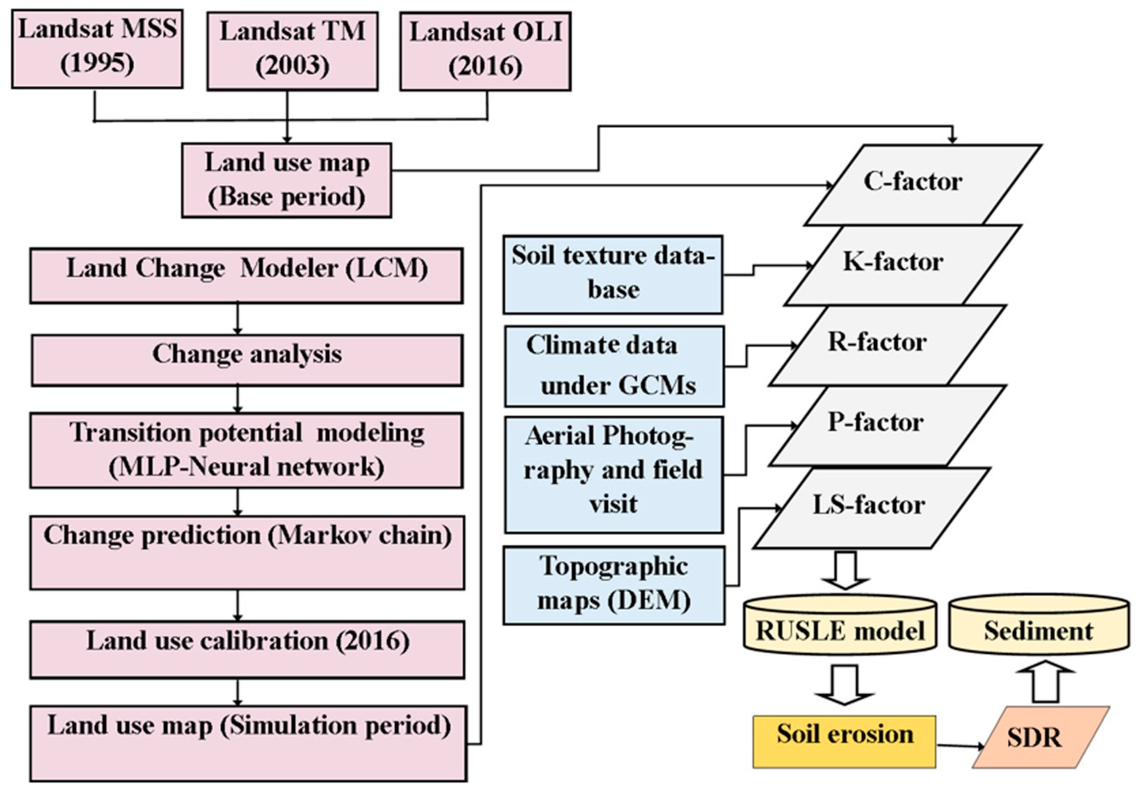
The present study involves three phases including assessing impacts of climate change on the R factor, the effect of land use change on the C factor and the effect of these two factors on the RUSLE equation and soil losses in the study area. RUSLE is an empirical erosion model designed to predict soil losses by runoff from a watershed [39,40,41], and is adequate for scenarios involving climate and land use change, erosion control practices and soil cover by vegetation [42]. It shows how climate, soil, topography and land use affect the surface soil erosion using the equation applied by Renard et al. [43].

As per previous research in different countries, R factor has a high correlation with soil erosion [44]. R is a numerical descriptor of the rainfall capacity to incite soil erosion and is based on maximum rainfall intensity [45]. This factor is calculated for different periods using the total rainfall kinetic energy and the maximum rainfall of 30 min. Given the lack of data on the watershed scale and the lack of all recording numbers from some rain gauge stations in the study area, the average annual rainfall and the Fournier index were used to estimate the R factor. As the results of previous studies suggested, the the Fournier index and rainfall erosivity are closely related [46] and can be used in regions without detailed data about rainfall intensity [47].

Therefore, the total annual rainfall was calculated after acquiring data from two meteorological stations inside the watershed area and three stations from its surroundings. The Fournier index was first calculated over each year and then the average was estimated. This means that first, the rainfall square of each month was calculated for each year and by dividing their total sum into the average rainfall of same year, the value of the Fournier index of each year was obtained. To obtain the average index of the station, the values of this index were averaged over the statistical period. Twenty-seven years of daily rainfall data for each station (1989–2016) was used to calculate the Fournier index. Using the inverse distance weighted interpolation method of in ARCGIS 10.2 software, the rainfall erosivity map for the whole basin was determined.

K denotes soil erodibility per unit of the rainfall erosivity index, which was determined using soil physical properties. In this study, 25 soil samples from different types of soil in the watershed area were collected and analyzed for the distribution of particle size, organic matter and hydraulic conductivity (soil permeability) using the standard procedures described in reference [48].

The slope (S) and the slope length (L) factors in the RUSLE model represent the impact of topography on soil erosion. The special impacts of topography on soil erosion were estimated by the LS (dimensionless) factor. In this study, the LS factor map for the study area was arranged in the ArcGIS 10.2 environment based on a flow accumulation map and slope map. The procedure is explained in detail by van Remortel et al. [49]. The slope and slope length were calculated based on the topography map (1:25000) provided by the National Cartographic Center of Iran.

Erosion control practice factor (P) reflects the decrease of soil loss on a field where any kind of soil conservation practice is performed (e.g., contouring, strip cropping, terracing, minimum tillage) as compared to the soil loss on the same field with upslope and downslope tillage [43]. Due to the fact that no soil conservation practice was performed in nonagricultural areas, the value of P was 1. For cultivated parcels, the P values were estimated using aerial photography and field observations based on the use and slope according to

Table 1. Attribute value of P factor for contouring and terraces in agricultural land based on Wischmeier and Smith [50].

Slope (%)	Contouring	Terraces
0–2	0.5	0.1
3–12	0.6	0.12
13–16	0.7	0.14
17–20	0.8	0.16
21–25	0.9	0.18

. In the Minab watershed, due to the large area that it covers, the P factor was only applied to areas with contour tillage and terraces.

Cover management C factor represents the effect of surface cover on soil erosion. As the soil cover increases, the risk of erosion decreases, thus the higher C value represents higher bare land area [40]. C factor estimation is differentiated between all land uses, therefore change in land use directly affects the soil cover (C value). Given that the purpose of this study was to predict the future of land use modifications, the use of the normalized difference vegetation index (NDVI) was not adequate for the RUSLE model and the C factor was derived from Land Use/Land Cover (LULC) map of the watershed and the values were determined based on previous studies [51,52,53,54]. The C factor values for each land use category were determined as 0.5 for rangelands, 0.31 for agriculture and 0.008 for forests. Urban land, water bodies and bare rocks were considered to have zero C factor value in this study. C factor was determined for 2030 from the land cover classes derived from the LCM model.

2.3. Land Use Change

In order to investigate and predict land use change (C factor) for a future period (2030), Land Change Modeler (LCM) was used and its results were compared with the baseline period. Land Change Modeler is software for creating ecological sustainable development that has been designed and developed to recognize the urgent and ever-increasing problem of land change and analytical needs of ecosystem conservation [55,56]. It is embedded in the IDRISI software but is also available as an extension in ArcGIS [57]. The Land Change Modeler provides a tool for evaluating and empirical modeling of land use change and its impacts [58]. Modeling was performed in three phases: (a) Change analysis (Map trend); (b) Transition sub models; (c) Land use change prediction.

In this research, land cover maps from 1995, 2003 and 2016 were introduced into the LCM for analyzing and detecting regional variations, and the extent of land use changes has been identified in these years. Landsat satellite images from TM 1995, ETM + 2003 and OLI 2016 sensors were used to evaluate land use change trends. ENVI 5.1 software (Exelis Visual Information Solutions, Boulder, CO, USA) was applied to analyze the satellite images. Supervised classification method of maximum likelihood was applied to prepare the land use maps. After classification, all land uses in the study area were classified into six classes (Bare rock, Agriculture land, Forest, Rangeland, Urban, Water body). Finally, monitoring of land use change in the past and its prediction for the future was performed using the Land Change Modeler (LCM) in TerrSet software (Clark Labs, Clark University, Worcester, MA, USA). Prediction of land use in 2030 was performed based on land use maps of 1995, 2003 and 2016 using the LCM model based on the multi-layer perceptron (MLP) artificial neural network.

The multi-layer perceptron (MLP) artificial neural network is an option in LCM that is used to model the selected transition variables. The MLP neural network needs to be trained with the back-propagation algorithm [59]. The variables were entered into the sub-model structure to run the model and the neural network generated cells for each of the selected transitions and then adjusted the weights to improve accuracy as the RMSE error decreases. In this part of the modeling, transition from one land use (e.g., rangelands) to another land use (such as agriculture) is modeled according to explanatory variables (such as slope, proximity to the road). This means that each pixel has a potential for the image to change from one land use to another. The output of this section will be a transition potential map for each change (for example, from rangelands to agricultural lands). To select the models that have the highest accuracy, it is essential that the model run multiple times with different scenarios.

After this step, five sub-models were considered for modeling transition potential using MLP artificial neural network. Transition sub-models were as follows: Rangelands to agricultural lands; Forests to rangelands; Forests to agricultural lands; Rangelands to urban lands; Water bodies to rangelands; Water bodies to agricultural lands. The explanatory variables used in LCM are the elevation, slope, aspect, distance from the road, distance from the river, and distance from the residential land, which have been used in most studies of land use change modeling (Figure 2).

The probability of transition to each land use was calculated using the Markov chain [60]. This model is run using the respective module in the software and validated. Then, the land use map for 2016 was simulated (Figure 3). The Kappa index was applied to determine the agreement between reference and simulated land use maps of 2016. The Kappa index expresses the agreement between two categorical datasets corrected for the expected agreement using a stochastic model of random allocation of class transitions relative to the initial map [61]. Kappa values close to 1 indicate greater compliance and values near 0 with less matching. If the Kappa index is appropriate, the 2030 land use map can be predicted.

2.4. Climate Change Scenario

In the present research, the observational data of the synoptic station of Minab and of its surrounding stations was collected and quality control was carried out on them. Then, Statistical Downscaling Model (SDSM 5.1) was used to downscale rainfall data in these stations during the baseline and future periods under the influence of climate change [62]. The statistical downscaling was performed by simulating local scale data based on Large scale atmospheric variables derived by the National Center for Environmental prediction (NCEP) reanalysis datasets (1961–2005) and a general atmospheric circulation model outputs (1961–2099) (Canadian Earth System Model: CanESM2) [63,64]. Downscaling precipitation was performed by the SDSM model in the following order: (1) preparation of predictand data and predictors; (2) data quality control; (3) selection of the best screen variables; (4) model calibration; (5) generation of future series of the predictand (precipitation data) [65].

To validate the performance of SDSM, rainfall was simulated using CanESM2 historical data from 1989 to 2005 and compared with observed data. For this purpose, model evaluation criteria of R², root mean square error (RMSE) and the mean absolute error (MAE) were used as suggested by Hassan et al. [66]. R² represents the relationship between observed and calculated data. The range of this parameter is between 0 and 1; values close to 1, indicating a strong correlation between the two groups. Low MAE and RMSE, values indicate a more efficient model for estimating climate parameters. RMSE and MAE are dimensionless (normalized) to compare different parameters with different units [67].

Following these steps and using future period data for the large-scale model, rainfall data for the 2016–2030 period was simulated under three scenarios. The scenarios were chosen from the Intergovernmental Panel on Climate Change (IPCC)—“Representative Concentration Pathways” (RCPs): RCP 2.6 (optimistic), RCP 4.5 (intermediate) and RCP 8.5 (pessimistic) as described by van Vuuren et al. [68]. Finally, the observed and simulated data were compared.

2.5. Model Running

After preparing factors required for the RUSLE model, all of them were logged into ARCGIS 10.2 software and erosion of the basin was achieved. Then, the erosion was converted into sediment yield based on the sediment delivery ratio (SDR). The estimated sediment of the RUSLE model was evaluated with actual sediment data for the baseline period, and then erosion was simulated under different scenarios of climate change (under the SDSM) and land use in the upcoming period.

In order to simulate the erosion intensity, the factors K, LS and P were assumed constant. In order to estimate the rainfall erosivity (R factor) in the upcoming period, at first, rainfall was generated under the RCP 2.6, RCP 4.5, RCP 8.5 scenarios using SDSM, and, after converting to the rainfall erosivity factor (based on the the Fournier index), was entered into the RUSLE model. In the case of C factor, a simulation of land use for the future period was made through LCM, and the C values to each land use were assigned based on previous studies. Finally, the C factor map was prepared and entered into the RUSLE model. With the change of C and R factors and constant consideration of other factors, simulated values of erosion intensity were obtained during the period.

Then, according to Ferreira and Panagopoulos [69], erosion was converted into sediment yield (Equation (1)), which is adequate for large watersheds and is using RUSLE data that was already calculated at the research area. In this study, the sediment delivery ratio was obtained according to the United States Department of Agriculture (USDA) method [54] (Equation (2)).

SDR = 0.51 A − 0.11

(1)

$$Sy={\displaystyle \sum }_{i=1}^n SDR* E$$

(2)

where SDR: Sediment Delivery Ratio, A: basin area (km²), E: Erosion (t ha⁻¹ y⁻¹), Sy: Sediment Yield (t ha⁻¹ y⁻¹).

3. Results

The land use maps for the three years 1995, 2003, and 2016 were prepared for the study area and presented in Figure 4. Kappa coefficients indicated that the accuracy of the produced land use maps was high in all years at 0.78, 0.86, 0.83 respectively. The overall accuracy of the maps was 85.5%, 91.7% and 89.8% respectively. As shown in Figure 4a, most of the area is covered with rangelands (56.8%), followed by bare rocks (33.48%), agricultural lands (7.37%), forest (1.5%), water bodies (0.57%) and urban environment (0.29%).

3.1. Transition Potential Modeling

Transition potential modeling from one land use to another was done using an MLP artificial neural network and

Table 2. Evaluation of artificial neural network (MLP) for transition potential modeling.

Sub model	Accuracy Rate	Training RMSE	Testing RMSE
Rangelands to agricultural lands	89.9%	0.0029	0.0031
Forests to rangelands	64.1%	0.015	0.017
Forests to agricultural lands	73.4%	0.0041	0.0043
Rangelands to urban lands	85.81%	0.00356	0.00361
Water bodies to rangelands	75.2%	0.023	0.024
Water bodies to agricultural lands	61.3%	0.01	0.014

present the results of the factors accuracy rate, training error and testing error that were determined for evaluation of transition potential modeling. Results in all sub models showed high reliability (61.3%–89.9%) and the ability of MLP to generate potential transition maps.

3.2. Land Use Prediction by Land Change Modeler (LCM)

Transition probability from one land use in 1995 to another in 2016 was calculated using the Markov chain. The highest transition probability was from rangelands to agricultural lands and from forest to rangelands (

Table 3. Matrix of transition probability from 1995 to 2016.

	Bare Rock	Forest	Rangeland	Urban	Water Body	Agriculture Land
Bare rock	1	0	0	0	0	0
Forest	0	0.85	0.13	0	0	0.02
Rangeland	0	0	0.67	0.01	0	0.32
Urban	0	0	0	1	0	0
Water body	0	0	0.03	0	0.97	0
Agriculture land	0	0	0	0	0	1

). Water bodies to agricultural lands transition area was very low and therefore it was omitted. The land use map for 2016 was simulated based on the changes that took place between 1995 and 2016.

Four kappa statistics were used for testing the accuracy of cells. The traditional kappa (Kstandard) was 0.895. A kappa for no ability (Kno) was 0.934 and two kappa to differentiate accuracies in quantity and location (Klocation and Klocation Strata) were both 0.961. The results of kappa showed that the used LCM had excellent ability to indicate grid cell level location of future change. After assuring the model’s performance in the prediction of land use map, the 2030 land use map was predicted using the Markov chain. Figure 5 shows the land use map for 2016 and the simulated map for 2030.

3.3. The Study of Land Use Change Trend Using LCM

Land use in the studied area was subjected to relatively significant changes. The area of each land use in 1995, 2003, 2016 and 2030 was presented in

Table 4. Land use areas in years 1995, 2003, 2016 and 2030.

Land Use	1995		2003		2016		2030
	km2	%	km2	%	km2	%	km2	%
Bare rocks	3553	33.48	3553	33.48	3553	33.48	3553	33.47
Forests	158.55	1.5	111.09	1.05	86.60	0.82	86.06	0.81
Rangelands	6029	56.80	5448	51.34	5169	48.72	5029	47.40
Urban lands	30.71	0.29	34.10	0.32	36.05	0.34	40.23	0.38
Water bodies	60.21	0.57	57.60	0.54	55.27	0.52	54.79	0.52
Agricultural lands	782.07	7.37	1409	13.28	1710	16.12	1793	16.90
Total area	10611	100	10611	100	10611	100	10611	100

. Those changes indicated that in 2030 compared to 1995, the area of agricultural lands and urban lands increased by 1011 and 9.25 km², or 129% and 30% respectively. Also, it was found that the area of rangelands, forest and water bodies decreased by 1000, 72.45 and 5.41 km², or 17%, 46% and 9% respectively, and bare rocks remained unchanged.

In the past the destruction of forest has led to the conversion of these lands into agricultural land and in some cases residential land, meanwhile the conversion of forest was relatively small size area and is expected to be conserved as it is. Therefore, the development of agriculture in the predicted period was derived mainly due to unplanned use of rangelands and their conversion to agricultural land.

Also, the results indicated that part of the vegetation cover would be destroyed in the future period due to forests being converted into agricultural lands (increasing the C factor) and rangelands being converted to agriculture (lowering the C factor in those areas). The C factor map in 2030 was produced according to those land use changes. The estimated P factor map of 2030 was created considering the values of Table 1. It was assumed that in 2030 all new cultivated parcels will apply contour tillage for slopes up to 20% and terraces for slopes above 20%.

3.4. Climate Change Scenario

The results of SDSM accuracy evaluation in downscaling of rainfall based on R², RMSE, and MAE indices at Bandar Abbas, Minab, Hajiabad and Jiroft meteorological stations are shown in

Table 5. CanESM2 model validation criteria for the period 2005–2015.

Station	MAE	RMSE	R2
Bandarabbas	1.34	2.09	0.96
Minab	0.38	1.51	0.91
Jiroft	0.08	1.28	0.93
Hajiabad	1.81	2.20	0.89

. The results showed that there is a strong correlation between simulated and observed values. The low RMSE and MAE values and the high R² values at all stations indicate that the SDSM model has an acceptable ability to downscale rainfall data and therefore, the model could be used to produce climatic data during the upcoming period.

Figure 6 illustrates the average observed and predicted rainfall under various scenarios at Minab station. The results show that rainfall during the future period under all scenarios will increase compared to the baseline (observation) period, and this increase is the highest under scenario RCP 2.6. The same pattern was observed at all stations surrounding the watershed area.

After predicting rainfall using the SDSM for the upcoming period, the rainfall erosivity factor was calculated under RCP 2.6, RCP 4.5 and RCP 8.5 scenarios based on the Fournier index for the 2015–2030 period. Figure 7 shows the rainfall erosivity factor derived from four stations of the study area and under different climate change scenarios. In general, we will see an increase in the rainfall erosivity factor in all scenarios in the upcoming period compared with the baseline period.

Figure 8 shows the rainfall erosivity map under the chosen RCP scenarios in the 2015–2030 period. The highest amount of R was observed under the scenario RCP 2.6 (34.2–40.6 MJ mm ha⁻¹ h⁻¹ y⁻¹). In fact, the results suggest that the amount of variation in the rainfall erosivity factor was related to the annual rainfall. The results of the investigation of the future rainfall erosivity factor indicated an increase in average annual rainfall at the watershed from 146.7 mm in the baseline period to 200.1 mm in the future period (RCP 2.6). Due to the increase in rainfall, the value of average rainfall erosivity factor changed from 28.78 6 MJ mm ha⁻¹ h⁻¹ y⁻¹ in the baseline period to 37.27 6 MJ mm ha⁻¹ h⁻¹ y⁻¹ in the future (RCP 2.6).

3.5. Erosion and Sediment Estimation Using the RUSLE Model

To prepare the average annual erosion map of Minab Dam basin, five generated layers include slope degree and length (LS), soil erodibility (K), conservation practice (P), vegetation cover management (C) and rainfall erosivity factor (R) were created in ArcGIS10.2 software (Figure 9). Using map algebra, the five layers were combined and the final soil erosion map at the Minab dam watershed in the baseline period was generated (Figure 10).

Erosion rate obtained from the RUSLE model was converted to sediment based on the sediment delivery ratio (SDR), before being compared with the observed sediment at the baseline period. The soil erosion rate in the study area was estimated with RUSLE at 10.64 t ha⁻¹ y⁻¹ and the estimation of sediment in the reservoir was calculated at 4.78 t ha⁻¹ y⁻¹ considering that the SDR was 0.45. Meanwhile, the average observed sediment at the Brentin sediment gauge station at the basin outlet was 6.2 t ha⁻¹ year⁻¹. From the above results, it was found that the difference between estimated and observed sediment was 1.42 t ha⁻¹ year⁻¹. In other words, the observed sediment content was about 22.9 percent higher than the estimated sediment. Therefore, it was assumed that that there was no significant difference between observed and estimated sediment, and thus, the RUSLE model had a relatively good performance and can be used for predictions of future scenarios.

According to the results of the soil erosion map (Figure 10), the largest part of the study area had low risk of erosion in the baseline period. The highest erosion was observed on marginal agricultural lands. By detecting the changes from 1995 to 2016, the share of each change in the production of erosion was determined. It was found that in the 21-year period of land use change, conversion of the forests and rangelands to agricultural lands had the highest impact on erosion (120 t ha⁻¹). Rangelands to urban lands generated 30.2 t ha⁻¹ and water bodies to rangelands, 0.67 t ha⁻¹.

By substituting two factors of rainfall erosivity (R) and vegetation cover management factor (C), and considering all other factors constant in the RUSLE model, soil erosion was predicted and calculated under different climate change scenarios: RCP 2.6 (optimistic), RCP 4.5 (intermediate) and RCP 8.5 (pessimistic). The results of the above simulations were presented in Figure 11. The results revealed that the highest average erosion during the future period was under the RCP 2.6 scenario, which was estimated at 14.5 t ha⁻¹ y⁻¹ in 2030. For RCP 4.5 was estimated at 12.8 t ha⁻¹ y⁻¹ and for RCP 8.5 was estimated at 11.4 t ha⁻¹ y⁻¹.

Prediction of sediment at the Minab dam watershed for 2030 under three climate change scenarios and considering the modeled land use change was 5.52 t ha⁻¹ y⁻¹ at RCP 2.6, 5.76 t ha⁻¹ y⁻¹ at RCP 4.5 and 5.13 t ha⁻¹ y⁻¹ at RCP 8.5.

Table 6. The relationship between the inputs of the RUSLE model and erosion rate.

RUSLE Factors	R2	Regression
R	0.69	E = 0.83 R − 143
K	0.47	E = 0.78 K − 103.6
LS	0.9	E = 0.95 LS + 271.5
C	0.95	E = 2.6 C + 356.1
P	0.2	E = 0.82 P + 47.2

shows the regression equation that presented the relationship between each of the 5 erosion factors (independent variables) and the erosion rate (dependent variable). The results are in agreement with previous study in Iran [70], showing that vegetation cover management (C) and topographic (LS) factors had the highest impact on the estimation of soil erosion, followed by the R factor of precipitation intensity.

4. Discussion

The results of the RUSLE model survey show a negligible difference between observed and estimated sediment in the baseline period, which suggests that this model has a relatively good performance in the field outlet sediment estimation. The advantages of using RUSLE in this kind of study include the following: (1) easy assessment of the soil management strategies and erosion control programs on erosion and sediment; (2) simple and fast analyses of the effects of climate and land use change on sediment; (3) easy integration in GIS for geographically precise analysis; (4) RUSLE has been extensively applied and tested over many years in different types of landscapes and climate and it is a well-known model. Meanwhile, the main disadvantage of RUSLE is that it does not have the ability to route sediment through channels [71]. Also, there are several sources of error in soil loss estimation using RUSLE, which include measurement error, spatial resolution of maps, slope length measurement error, and the grid size of DEM [72].

The results of the combination of effective factors in erosion showed that soil erosion is most associated with the C factor, followed by LS and R factors, which is in accordance with the results of El Jazouli et al. [73]. This means that land uses with low and poor density of vegetation cover have the maximum amount of C factor and the greater risk of erosion.

As the results revealed, the highest amount of erosion was the result of the conversion of rangelands to agricultural lands due to reduction of soil organic matters and increased soil compaction that was also observed in the results of previous studies [74,75]. Another land use change that has had a great effect on erosion is the conversion of forest into rangelands and agricultural lands that has also been observed in studies by Mancino et al. [76] and Wynants et al. [77]. Meanwhile, Latocha et al. [78] found that land abandonment may increase soil erosion to a larger extent than climate change.

In this study, the conversion of rangelands to agricultural lands was observed on the margin of agricultural land, which indicates the development of agricultural lands towards the degradation of rangeland [79]. Moreover, a large part of the future land use/land cover change was the conversion of forests into agricultural and rangelands, thus, it was found that erosion rate in the study watershed will increase due to change in LULC as a result of increased C factor. The conversion of rangelands to agricultural lands causes a significant reduction in soil organic matter content and soil nutrients [80], while land-use change from arable lands to orchards can reduce soil erosion and increase nutrient loss [81]. Also, cultivation and plowing operations may led to the breakdown of soil aggregates and the destruction of the soil structure [82].

Elimination of rangeland vegetation cover, or tree cutting followed by unsuitable tillage, reduces organic matter and destroys the soil structure, thus increasing runoff and erosion [83]. Moreover, excessive grazing compacts the soil, reduces infiltration, and increases runoff, erosion and sediment yield [84]. If those land use changes will not be supported by soil conservation measures, especially in the watershed areas with sharp slopes, soil erosion may decrease the lifetime of the reservoir, with serious consequences for the stability of the region.

The results of various RCP scenarios showed that all three climate change scenarios predict an increase in rainfall erosivity, which is consistent with the results of Zhang et al. [85] and Litschert et al. [86]. In all climate change scenarios, the model showed an increase in precipitation during the winter months in the Minab area. The RCP 2.6 scenario had the highest amount of rainfall erosivity factor and therefore had the highest erosion rate, followed by RCP 4.5 and RCP 8.5. Compared with the baseline period R factor, the erosion rate will increase in 2030. A similar increase of soil erosion due to climate change (an R factor increase) was observed under different climate conditions in China [85], USA [87], Ireland [88], Thailand [89] and north Iran [90], which was confirmed in the present research for the subtropical desert climate.

5. Conclusions

The study shed light on upcoming impacts of climate and land use change on soil erosion at the Minab dam watershed. The Minab dam was constructed in a region with a high risk of desertification and a typical subtropical desert climate. The watersheds of the Persian Gulf are known to have significant soil erosion problems. Many Middle East countries with similar climates may use the results of the present study to apply policies of sustainable land use change that will help with adaption to ongoing climate change.

The result of combining different scenarios of both land use and climate change indicated the increase of soil erosion in all scenarios. The highest mean annual erosion was estimated at 14.5 t ha⁻¹ y⁻¹ under the RCP 2.6 scenario. The land use changes reported in this study show conversion from forest and rangelands to agricultural lands, revealing high pressure to forest land and risk of land degradation. The highest erosion was observed on marginal agricultural lands in any of the RCP scenarios, while forest and low slope agricultural land had the lowest erosion. The results indicate that due to the increase in rainfall and, consequently, the increase in the rainfall erosivity (the R factor), and also due to change in the C factor, soil erosion will increase. This may lead to an increase of sediment in the reservoir from 4.78 t ha⁻¹ y⁻¹ in 2016 to 5.52 t ha⁻¹ y⁻¹ (at RCP 2.6) in 2030 and decrease the lifetime of the reservoir.

If this trend continues, this will affect the life of millions of people because the reservoir provides cheap water to many farmers and people of the Hormozgan province. However, P factor has the potential to maintain soil erosion under control, or ever reverse the tendency if sustainable soil management will be applied to all newly converted agricultural land. The present study shows the urgency for precise agro-environmental policy that will protect land at risk of erosion by improving the C factor, and recover part of the degraded land by improving the P factor. It is mainly the margins of agricultural land that where most land use changes are expected to occur in future years. Climate change is almost unavoidable. Hence, if land use change is controlled by promoting sustainable land use policy and reservoir managers prevent expanding intensive agriculture use in this vital watershed, soil erosion can be greatly controlled and even reduced despite the future climate change risks. The above can be further enhanced by taking measures for soil conservation practice (contouring, strip cropping, terracing, minimum tillage) at the hotspots of the watershed where there is higher risk to soil erosion. These findings provide valuable information for watershed managers and policy makers in planning sustainable development of the region.