Abstract
Green infrastructure plays an important role in recreation and human well-being, especially in urban and peri-urban areas. Our study aimed to evaluate and map the recreational potential of an urban area (Brașov, Romania) using two data sets: (a) people’s preferred landscape features and (b) preferred locations where outdoor activities and recreation take place. The latter was gathered through participatory mapping techniques. For each location, we computed explanatory variables, e.g., the distance to 19 landscape elements known to be important for recreation. Based on (b), we determined the recreational activity profiles for each participant and evaluated how well these profiles matched the participant’s preferences for landscape features (dataset a). Finally, recreational potential was mapped by computing a recreational index using dataset b. Two preference profiles (P1: urban, infrastructure-oriented; P2: nature-oriented) were identified based on people’s preferred landscape features, and three recreational activity profiles were identified based on the preferred locations, i.e., an “urban”, a “nature”, and an “ubiquist” type. The importance of green infrastructures for recreation in both preference profiles was striking. Many persons belonging to the urban and infrastructure-oriented group indicated that they recreate in locations with a high amount of green infrastructure and nature. The map of the recreational potential shows hotspots for recreation but also areas lacking recreational provisions, giving useful insight for future urban planning.
1. Introduction
The recreation potential is—among other factors—strongly dependent on green infrastructure (hereafter referred to as GI). The latter has become a useful tool for the management of cities and is a popular subject in European policy regarding urban environments [1]. The term GI has been used very broadly by city planners and ecologists (see, e.g., the definition-oriented paper by Garmendia and coworkers) [2]. It ranges from restored habitats in cities, green roofs, parks, and forests to urban plazas, just to mention a few. Ecologists consider every green space that supports biodiversity as GI, whereas recreation planners also subsume natural elements linked to vegetation as being GI, such as water, infrastructure like nature trails, fitness courses, and benches, in other words, everything that enables people to link to vegetation when outdoors. In our paper, we use this broad definition of GI and include all patches with vegetation as well as infrastructure or natural elements that have clear links to these patches and support people’s well-being when outdoors. This definition is in line with the EEAs (European Environment Agency) definition [3], which clearly suggests that GI is not restricted to inner cities but reaches out to the peri-urban and even the rural area. As shown in a recently published review article [4], GI is beneficial for a wide range of ecosystem services and is highly relevant to health [5]. Here, we give a list of three benefits of GI which are highly relevant to the topics of our paper. The list is not complete. For a full list, we refer the reader to [4].
Recreation (CICES—Common International Classification of Ecosystem Services—cultural services): Most urban recreational landscapes comprise urban green infrastructure elements [6], for example, parks, public gardens, or urban forests [7]. The implementation of GI has been shown to positively change the quality of life in urban areas worldwide [8,9]. GI can help to improve human well-being, both from physical and psychological perspectives [10], especially in urban areas where the demand for such recreational spaces is increasing [11,12]. Green spaces offer opportunities for relaxation and stress relief [13] and influence health behaviors (physical activity, social interactions, mental health) [14]. Green spaces are also positively correlated with the perception of people’s health, especially for the demographic groups of elderly and young people and people with a secondary level of education, who spend much of their time close to their place of residence [15].
Climate mitigation and adaptation (CICES regulating services): GIs assist in the mitigation of climate change effects [16,17] as an adaptive response to changing environmental conditions [18]. The function of cooling and shading, provided by certain types of GI (e.g., urban woods, trees), is not only important for recreation but also reduces life-threatening heat stress impacts [19] and contributes to urban resilience against phenomena such as the urban heat island [20].
Identity building (not a CICES service but important in connection with recreation): As parts of the urban landscape, GIs not only provide aesthetic and recreational benefits, but they also contribute to the urban identity which embodies natural and cultural elements [21,22,23]. These are cases where a landscape becomes valuable by playing an active role in the creation of shared values [24] or meanings that social groups attribute to its features. This place bonding requires long-term usage for such bonds to form [25].
These selected benefits are a result of both the physical presence of GI and people’s perceptions and interpretations of GI within the landscape. A better understanding of this dualism can be found in the space-place theory [26,27]. This theory is essential for understanding how people perceive and experience landscapes: The space component concerns biotic and abiotic elements (natural and man-made) of locations and builds an essential basis for the way people perceive and interact with landscapes. The place component emphasizes the individual and cultural connections of people with landscapes and particular places. This progression from landscape as a physical support to a landscape with a meaning is based on the attachment of social values—perceived values that people ascribe to the ecosystem services they receive (e.g., cultural values, recreational values, space, and freedom) [7]. Relational thinking in landscape research is a new approach for addressing sustainability challenges which sees the landscape together with the relations established in it (social relations and preferences of single individuals or social groups) [28]. The landscape gains cultural and personal meaning which helps in shaping the landscape experience, a vital aspect in recreation [29]. Often this implies the accumulation of an individual’s experiences, which forms the basis of the transition of an area from a “space” to a “place” [30,31].
Place attachment plays an important role when it comes to recreational resources, as it enables people to establish bonds and define the recreational quality of a place [25]. Sometimes, place attachment can be the solution to maintaining the identity of an urban area [22]. It is linked to the health of the community, or more specifically, to the perceived quality of life [25], as it is a reflection of the relationship between humans and landscapes [32,33]. People perceive the benefits of GI as an integral part of their experience. However, while they want to feel the authenticity of natural environments, they also desire order and accessibility [8]. GI characteristics such as condition, accessibility, and safety can influence people’s perceptions regarding a certain space and thus, how much time they choose to spend there for leisure or physical activity [34,35] and the types of social values they attach to it [7,36].
Within landscape research, the concept of space and place is often used along with mapping methods to assess preferences for landscape features, access to locations that individuals have developed an attachment for, or when dealing with landscape transformations [32]. This leads to an improved understanding of the recreational potential of urban landscapes, assisting future planning of urban green infrastructures [9]. This can be beneficial when designing neighborhoods with easily accessible and easily understandable park areas. Mapping links the physical/geographical dimensions of places [37] to shared values or meanings. The mapping of “special places” can give insight into the relationship between people’s place attachment and shared values [38,39]. Using data in both point and polygon form, this method integrates qualitative aspects with spatially explicit locations [40].
A popular method to address the provision of ecosystem services and goods is distance decay analysis [41,42]. Previous studies assessing how people use green areas have implemented physical indicators based on distances [34,43], travel time, and modes of transport [44]. Combinations of these variables can be used to predict the use of recreational areas, for example, by analyzing distance-weighted landscape properties such as paths, recreational infrastructure [45], residential areas, water bodies, built space, roads, and green areas [46]. Most recommendations for the planning of recreational areas consist of distance thresholds, for example a 500 m [47] or 5–10 min walk from a residence [48].
Studies on outdoor recreation often focus on a user’s landscape preferences and their attitudes [36,48,49], the latter being important factors that shape recreation patterns. People’s preferences can also serve as a proxy in the process of mapping recreational potential [6]. Some studies have used an expert knowledge approach to determine the relevant factors for recreation planning [36,50], and some have used community knowledge through participatory mapping [51]. Most studies have examined the landscape properties found in the immediate surroundings of recreational hotspots and only few analyses have taken into account how the landscape context at a site affects the recreational potential. This lack of knowledge on how people value landscapes and their integration into planning has great impacts on decision-making processes and can result in the development of resource management conflicts [45,52].
Given the aforementioned knowledge gaps, this study aims to evaluate and map the recreational potential of an urban area using people’s reported preference patterns for landscape features and locations. The paper contributes, through its case study, to the existing literature on the topic of recreation in Eastern Europe. These are the main objectives:
- (a)
- To determine people’s preferred landscape features when outdoors;
- (b)
- To evaluate the participants’ recreational activity profiles based on their preferred locations;
- (c)
- To link (a) and (b) and determine the role of green infrastructure in people’s recreation patterns,
- (d)
- To map the recreational potential using the preferred locations of the participants and distance-weighted landscape features as explanatory variables.
A further aim of the paper is to provide the stakeholders involved in the decision-making process and policy making around GI with a broader understanding of how recreational values can enter the urban planning realm.
2. Materials and Methods
2.1. Study Area
Brașov is a Romanian city (Figure 1) with almost 294,000 inhabitants [53] that is located in the biggest valley of the Carpathian Mountains. It has a relatively flat topography in the north and a mountainous part in the south dominated by the Postăvaru Massif, which reaches 1799 m at its highest peak. Brașov has an extended urban forest, a mixed forest with coniferous species such as spruce (Picea abies) and firs (Abies sp.) as well as the deciduous species European beech (Fagus sylvatica) and sessile oak (Quercus petraea). There is also an IUCN (International Union for Conservation of Nature) protected area (Category IV), Tampa Mountain. Due to its green infrastructures, the city of Brașov can provide many opportunities for recreation, both within the city and in its surroundings. The geography of the area has always been part of the urban history and identity that makes Brașov an attractive tourist destination for both national and international visitors.
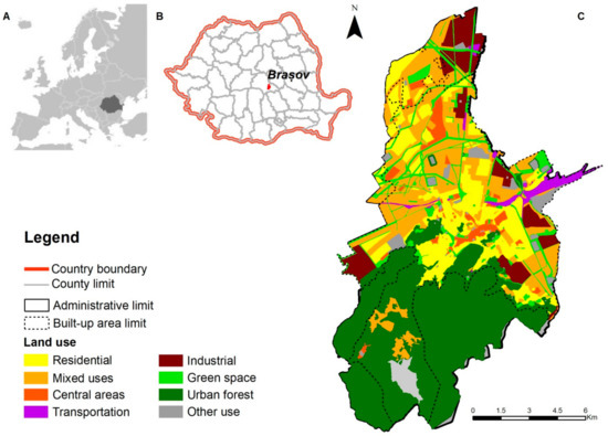
Figure 1.
Study area. (A) Localization of Romania in Europe; (B) Brașov city is indicated on the right as the red area on the map of Romania; (C) Brasov city’s land use map based on the masterplan.
2.2. Methodological Workflow
Our methodology consisted of three major stages, which are described in the next subsections. The first stage was the data collection process which used a participatory approach. The second stage consisted of two principal component analyses (PCA) that sought to determine and evaluate users’ recreational profiles. The third part was the computation of a recreational index to help in the mapping of the recreational potential for Brașov. The methodology workflow is displayed in Figure 2.
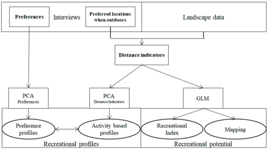
Figure 2.
Methodology workflow.
2.3. Data—Participatory Approach
This study was based on people’s preferred landscape features and locations for recreation inside Brașov’s administrative area. In order to map the recreational potential, we recorded two main types of data: (a) people’s preferred landscape features and (b) spatially explicit preferred locations when outdoors. This data was gathered via face-to-face interviews (N = 75) which took place in different areas of Brașov: small neighborhood parks, the city center, or recreational areas. Interviews comprised two components: a questionnaire and a participatory mapping exercise.
In part (a), we gathered data regarding social statistics: age group, gender, level of education, and employment status. Participants were asked how long they had been living in Brașov and what neighborhood they lived in. Participants were only asked to specify the name of their neighborhood, as we observed that people were reluctant to answer when asked about their home address during interviews. We restricted our sample to residents of Brașov, as we focused on close-by recreation during weekdays and weekends and not on tourism activities. The subsequent questions addressed the participants’ recreational behaviors: when they usually spend time on recreation, what means of transport they use to get to the area of their recreational activity, and how often they visit Brașov’s forests for recreational purposes. An important part of this interview phase was the participants’ preferences for different landscape features, e.g., forests, water bodies, monuments, parks, etc. We asked the participants the question “How much do you prefer the following elements in the landscape?”, and we presented a table with a list of elements (forests, water bodies, sunny spots, etc.). People expressed their preferences on a Likert scale, a common instrument in social science research [48,54], ranging from 5 (“I like it the most”) to 1 (“I do not like it at all”). All landscape elements included in this part of the questionnaire can be found inside the study area. We considered the answers that we received as preference variables in our study.
In part (b) of the interview, we asked participants to draw points on a paper map to indicate locations that they prefer because—in their opinion—they have a high recreational value. Each participant was allowed to point out a maximum of five locations. These places were considered the most relevant for people’s perceptions. They know and probably utilize them, and they therefore speak from their real-life experiences of recreating at these places, even if they extrapolated to areas that they do not necessarily engage with. In this case, the perceptual and actual are tightly connected. We randomly selected our participants from different locations of the city where the interviews were carried out. A total of 191 geographically referenced locations were recorded, with participants recording an average of 2 locations each.
Landscape data for these locations were collated from different sources: the local administration (providing the city’s master plan, the urban strategy and other planning documents) and the forestry department (providing forest management plans). Further useful information for the current research came from volunteered geographic information (VGI), an important data source whose purpose is to collect and share free geographic data. These tools can fill data gaps with local knowledge, especially when it is linked to recreation [55]. The Open Street Map (OSM) project is one of the many VGI initiatives that have developed in recent years. We used the OSM database to add spatial information about urban landscape features, i.e., the road system and building footprints. These data were updated using aerial images (from the year 2008) with 5 m resolution provided by the National Agency of Cadaster and Land Registration.
2.4. Evaluation of Recreational User Profiles
For each participant, we determined two profiles: (a) a preference profile for landscape features and (b) a recreational activity profile based on the locations where he/she expressed high recreational values.
For (a), we carried out a PCA using the stated preferences for landscape features of each participant. Sixteen landscape features, rated on a Likert scale, were included as variables in our analysis [56] in order to have a more detailed picture of which elements users prefer in the place they recreate. In both PCA analyses, we selected the number of components based on their eigenvalues which were compared with a Monte Carlo PCA parallel analysis [57]. To assign the specific preference profile to each participant, we calculated PCA scores and assigned the profile which corresponded to the component with the highest score.
For (b), rather than analyzing the landscape quality at specific locations, we conducted a distance decay analysis to generate a more comprehensive picture of perceived recreational values. For each preferred location indicated in the interviews, we computed the distance to 19 landscape elements, some of which were known to be recreational drivers. We used the “near” function from the analysis tool “proximity” in ArcMap, ESRI software ArcGIS 10.3 (ESRI, Redland City, California, USA) to calculate the Euclidean distance between preferred locations and these landscape elements.
The novel aspect of using distance data between locations and landscape features instead of landscape features at the exact site is that we were able to consider the entire landscape context of a site. In other words, if, for example, a certain preferred site was located in the forest (distance to forest would be 0), its recreational value was not only “forest” but was equally determined by distances to water, road, recreational facilities, etc. This contextual information, expressed by distance, is important for users, because the quality of a place is not only determined by what is there, but also by what is near or far to it. Table 1 presents the distance indicators and their data sources.

Table 1.
Distance indicators.
We analyzed distance indicators for each mentioned location in order to identify clusters and groups of variables and to reduce the dataset while keeping as much information as possible. To avoid collinearity in the data, we reduced the number of distance indicators in the analysis from 19 to 10 by examining the correlations between them. We excluded variables with the majority of correlation values lower than 0.3 or higher than 0.9 [57] in order to focus on clusters of variables and minimize the redundancy in the data. We are aware that this approach has a certain degree of subjectivity. A PCA was conducted to highlight specific recreational activity profiles. To compute the PCA, we used R software, version 1.0.44 (University of Auckland, New Zealand), using the “principal” function in the package “psych” with an oblique rotation. To assign each participant a profile, we obtained PCA scores for each location. As one participant could be linked to several locations, we averaged the scores of the locations linked to the same participant to transform the dataset from location level to participant level. Each participant was then assigned a recreational activity profile based on the component which attained the highest average score.
To link users’ recreational profiles, after assigning the two profiles to each participant, we superimposed them to see if the stated landscape preferences matched the activity profiles of the visited locations.
2.5. Mapping Recreational Potential
Recreational potential was modelled using the distance indicators as explanatory variables and the locations where participants reported high recreational values. We computed an index of recreational potential by fitting a GLM (Generalized Linear Model) with a binomial distribution. The latter was driven by presence/absence points (locations). As absence points were not recorded in our study, we generated them by computing 150 random pseudoabsences (2 for each participant in the survey based on the average number of locations specified by participants). These absence points were considered as having no recreational value for participants. The method of assigning pseudoabsences is described widely in the literature, e.g., by Lütolf et al. [58]. We then considered the perception of recreational value as a response variable formed by a series of vectors of 0 and 1. The points where participants indicated perceived recreational value in the landscape were assigned the value 1 and the randomly generated points (the background), which were considered without perceived recreational values, were assigned the value 0. We assumed that this response variable was binomially distributed (Bernoulli distribution) [59]. The resulting dataset consisted of a layer of 341 points, either indicating a recreational potential or a lack thereof.
The explanatory variables in our model were the same distance indicators as those used in the PCA analysis. The fitted probability for occurrence at any selected point was interpreted as an index of recreational potential. The model’s goodness of fit was evaluated by calculating the root mean-square error (RMSE) and the mean absolute error (MAE) and by visually displaying the fitted values against the observed ones [59]. The index of recreational potential had values between 0 and 1, with 0 signifying no recreational potential and 1 signifying the highest recreational potential. Based on the the values predicted by the model, which were computed using the “predict” function in R software, we mapped the recreational potential. We used the “spline” function in ArcGIS software to interpolate the index of recreational potential and to obtain a surface type map.
3. Results
According to the demographic data collected for our sample, both genders were equally represented in the interviews with a slight majority of men (53%). Forty percent of the participants were young people aged under 25, followed by the age group of 26–39 years old (29%). The age group 40–60 years old represented 24%, and roughly 7% of participants were over 60 years old. Fifty-three percent of the participants had studied at university, and 40% had completed high school educational programs. Eighty-five percent of the participants had lived in Brașov for over 10 years, and 72% stated that they do close-by recreational activities throughout the week, both on working days and at the weekend. Most of them leave directly from home to go to recreational areas (80%), with the second most popular origin for this trip being the workplace. In terms of the means of transport to recreational areas, many participants preferred only walking (40%), 14% used their own car, 12% took public transport and walked, and 10% reached recreational destinations using just public transport.
3.1. Recreational Profiles
A first, PCA was applied to the 16 variables which depicted people’s preferences for different landscape elements on a Likert scale (ranging from 1 to 5). The Kaiser–Meyer–Olkin (KMO) test had a value of 0.61 and the Bartlett’s test for sphericity χ2 (120 df) had a value of 389.7399 (p < 0.001), indicating good analysis performance [57]. In this case, we chose to extract two components (P1 and P2) based on their eigenvalues. These components explained 39% of the variance in the data regarding preferences for landscape features. We interpreted these components as two profiles of recreation based on landscape preferences: preference for an urban environment (P1) and preference for a natural environment (P2). The loadings are displayed in Table 2.
Table 2.
Results of the principal component analysis (PCA) structure matrix for people’s preferred landscape features; loadings are displayed for components P1 and P2.
We used the PCA scores obtained for the two extracted components (P1—preference for an urban environment and P2—preference for a more natural environment) to see if there were any significant statistical differences between gender or age groups based on which component they scored higher on. Both component scores presented a normal distribution, based on the Shapiro–Wilk test (P1: W = 0.969, p = 0.06; P2: W = 0.976, p = 0.17). The Levene test showed that the component scores presented similar variances for gender (P1: F = 2.50, p > 0.05; P2: F = 0.28, p > 0.05) and also for the age groups considered (P1: F = 0.026, p > 0.05; P2: F = 2.77, p > 0.05). Women registered a mean score of 0.13 for the first component (P1), while men had a mean of 0.11. The differences were, however, not significant (t (64.6) = 1.07, p > 0.05) with a small size effect (r = 0.13). For the second component (P2), men scored, on average, higher (mean of 0.07) than women (mean of −0.08); again, this difference was not statistically significant (t (69.12) = 0.64, p > 0.05) with a small effect (r = 0.07).
A second PCA was applied on the remaining 10 distance indicators using an oblique rotation method which allows correlation between factors. The KMO test for sampling adequacy recorded a value of 0.68, which is higher than the acceptable limit of 0.5. Bartlett’s test for sphericity (χ² (45 degrees of freedom, df) = 1107.954, p < 0.001) indicated that the correlations between the distance indicators were sufficiently large to perform a factor analysis. We chose to extract three components hereafter referred to as D1, D2, and D3, which explained 75% of the variance of data and had eigenvalues higher than Kaiser’s criterion of 1. Table 3 shows the structure matrix with the highest loadings for each variable.
Table 3.
Results of the PCA structure matrix applied on distance indicators. The D1, D2, and D3 components and their highest loadings for each variable are displayed.
By analyzing how variables clustered around the resulting components of the PCA, we interpreted each component as a recreational activity profile on the selected locations. The first component (D1) was characterized by a strong presence of urban structures (residential areas, paved roads, historic buildings); hence, it was termed “urban recreation”, which means that the participants opting for these sites consider urban structures to be ideal elements for recreation. These can be shopping activities or activities of urban life. The second component (D2) was related to a more natural environment (urban forest and paths), and we considered it as nature recreation, where the person perceives more natural places to be adequate for recreation. These places, which are perceived as having high natural value, are frequently at the city’s edge. Urban green does not load in this profile. The third component (D3) was interpreted as a mixture of the first two profiles, as both distance to buildings and distance to urban green areas had high loadings. We labelled this component ubiquity recreation, because it combines urban features with more natural spaces.
We compared the PCA scores of the two profiles for each participant. The results are shown in Table 4. The participants who scored high on component P2 (preference for natural environments) correlated with a high score on component D2 (recreational activity profile “nature recreation”). Their percentage (23%) was higher than in the other two activity profiles: D1 (urban recreation, 12.2%) and D3 (ubiquity recreation, 16.2%). Nonetheless, people who scored high on P1 (urban preference component) also showed a considerably high share in the nature recreation profile D2 (18.9%), even higher than in the urban recreation profile (D1, 16.2%). This highlights the fact that green infrastructures have high importance for recreation, even if people have a preference for a more urban lifestyle (profile P1). The fact that the ubiquity recreational activity profile (D3, 28.7% of all participants) and the nature recreation profile (D2, 41.9%) made up more than 60% of the respondents, once again underlining the importance of green infrastructure for people’s recreation.
Table 4.
A comparison of PCA scores on preference profiles is indicated in the two rows, and three recreational activity-based profiles are shown in the columns.
3.2. The Index of Recreational Potential
As described in Section 2.4, we fitted a GLM with a binomial distribution to model and predict occurrence of places where participants express high recreational values. The GLM yielded regression coefficients for every explanatory variable (see Table 5). Note that the explanatory variables represent distances to landscape features (distance to paths, distance to recreational forests). Thus, a negative sign of Beta indicates a positive effect on the index and vice-versa. Accessibility (distance to roads, paths, buildings, residences) was shown to play an important role as well as close-by forests and recreation attractions. This is well in line with [39] and confirms them as important drivers of recreation [60,61]. Urban green, historic monument mixed-use areas showed positive Beta values, indicating that their influence on recreation is negative. This shows that, averaged over all respondents, nature recreation outside the city is the preferred mode.
Table 5.
Multiple regression coefficients: B, SE, and Pr (N = 341).
Figure 3 graphically represents the goodness of fit for our model. This model had two random factors: the age group and the gender of the participants. The model underestimated the small index values (0.2–0.4), overestimated the medium values (0.4–0.5, 0.6–0.7), and fitted the higher values (above 0.85) best. We interpreted these higher values as places which are perceived as having “high recreational value”. The AIC (Akaike information criterion) value from the model was 266.03, the RMSE (root-mean-square error) was 5.53, and the MAE (mean absolute error) was 2.91.
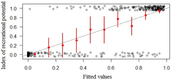
Figure 3.
Fitted values of the model depicted as red points with bars representing standard deviations. The dotted line represents a perfect prediction of the observed values. The dark points are observed values—places where recreational value is perceived (value of 1 for the index) or where it is not (0 value).
Mapping the recreational potential highlighted the urban forest edge and areas surrounding it as having the highest index value for recreation (Figure 4). Through applying GLMs, we obtained an index of recreational potential, with high values indicating that we would expect many people to consider the area as valuable for recreation, and low values indicating that only a few people would select the area as having a high recreational potential for them. The map clearly shows an imbalance between the north and the south parts of the city, caused by the absence of forests in the north and a dominance of positively loading (Beta) elements such as management areas, mixed-use areas, etc. The farther away these features are, the better for recreation.
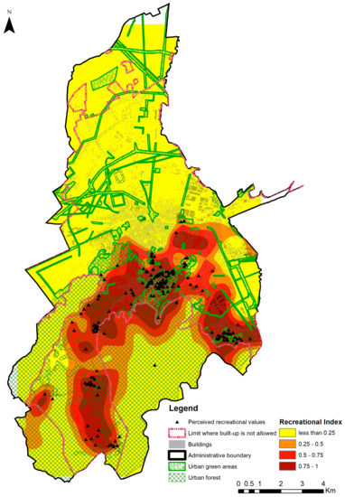
Figure 4.
A map of the city of Brașov showing the spatial distribution of recreational index values.
4. Discussion
This is one of few spatially explicit recreational potential analyses that uses distance data from landscape features and not the landscape features themselves to explain people’s preference patterns for recreation activities. The interesting aspects of our model and how they relate to the current state of knowledge are outlined below.
The distance decay indicators revealed three recreational activity profiles based on the preferred locations when outdoors. The “urban” recreation profile (D1, see above) is linked to elements such as historic buildings and developed infrastructure, characterizing mostly central areas where accessibility is higher and urban leisure activities are present, e.g., shopping or strolling. The strong effect of accessibility is also visible in the GLM and confirms other research suggesting that people’s route choice for recreation is often based on a short path strategy inside the city and becomes a combined strategy with trade-offs between quick access and a high quality route when distance increases [49]. On the other hand, the nature recreation profile (D2, see above) in our study is in line with other studies focusing on the spatial locations of visited recreation areas [34,62]. This profile identifies a dominance of recreational activities in natural areas such as forests, woodlands, and open space areas around cities. The third type of recreational profile, “ubiquity recreation”, was interpreted as a mixture of the first two profiles—a way of satisfying the need to recreate in a more natural environment while remaining close to urban life. Only in this profile does distance to green urban areas have a high influence, whereas for the others, it does not play an important role. Based on these findings, we mapped the recreational potential of the city of Brașov for the average user, creating a useful instrument for future planning. The use of geodata and its connection with human perception is a popular method, as recent literature shows. Like in our research, it leads to results that can support and influence GI policies in urban areas. Our results provide useful insight for future urban development strategies by geographically referencing how the local community assesses their environment from a recreational perspective. This type of information can determine whether a project fits the landscape, or not or how well it is received by people, to avoid potential future conflicts.
In a further part of the analysis, based on participants’ preferences for selected landscape features—not places—we obtained two types of recreational preference profiles. The P2 component (preference for natural environments) is linked to nature-based recreation such as walking and nature observation in larger habitats such as forests. The first preference profile (P1—preference for urban environments) is characterized by recreation which is concentrated in a specific area, requiring infrastructure and often linked to socializing. These two profiles are completely in line with other studies. Profile P2 confirms studies highlighting the recreational potential of forests, in particular, urban forests [63,64,65] and natural areas outside cities used for walking, hiking, and mountain biking. Profile P1 exhibits the growing number of people that enjoy city life in cities that try to improve, e.g., pedestrian arcades or green infrastructure.
One of the major findings of our study is that the participants classified into the P2 profile (preference for natural environments) do indeed seek places with more natural elements (D2 profile). Surprisingly, the urban group (P1) with clear preference for city life also seeks places with nature elements (D2), emphasizing the important role of green infrastructure, even for city people. This finding becomes imperative when planning large residential areas at the edges of cities [66,67]. With increased urban cover, nearby outdoor recreation areas might become a scarce resource with crucial impacts on people’s well-being [43,48]. One of the challenges generated by the imbalance between urban densification and the sprawling of cities is the decrease of “common” green infrastructure outside cities such as agricultural fields, forests, meadows, etc. This decrease can increase the pressure on the existing green spaces due to recreational demands [68,69]. Our analysis with the recreational profiles could be used by city planners; they could develop demand-based development of green infrastructures, where urban green for the “ubiquists” would be generated, forests for the nature-loving would be maintained, and attractive urban centers for the “urbanists” would be planned.
In our study, participants who showed high preferences for urban features also preferred sites with high nature potential. We do not know whether they are active users of these places or just indicated where—in their opinion—“nature” could be found. If the latter is the case, it might indicate that people can develop an attachment to a certain space, even though they have never visited it, by giving it a symbolic value and transforming it into a place [25]. For this group, the outskirts of the city, occupied by Brașov’s urban forests, could indeed play the role “longing for nature”.
When thoughtfully planned, GI can contribute towards urban development which takes nature conservation into account and can also promote public health [9]. “Collaborative planning” [70] implies that landscape changes must be precursors to added value, which may often develop into the provision of multiple ecosystem services [71]. This aspect not only helps us to understand how the urban community perceives and uses this recreational potential but also how this potential can be easily integrated into tourism activities. Our findings support those of Gundersen and coworkers [63], highlighting the necessity to develop multiple-use planning tools to provide good access to recreational activities in urban forests which serve as “hotspots” for ecosystem services. Our results identified that quite a large portion of people are "ubiquists" when outdoors. Old parts of the city and urban green space are important for them. These results confirm the fact that central areas must have a good supply of cultural and habitat services to be attractive and that everything should be undertaken to maintain these services and reduce the risk of well-being decreasing as a result of urbanization [72].
In cities, quality of life is directly related to cultural services and social benefits that are found in the urban landscape. People involved in interactions with urban green spaces in the wider sense have generally reduced stress factors, which has become an important indicator for assessing the quality of urban areas [73].
These results provide a useful insight into the recreational potential of the urban area of Brașov. This not only helps the city administration to develop urban strategies, but also helps the forest administration to adapt forest management practices to the public’s expectations of recreational areas.
4.1. Limitations of the Study
We identified some limitations of our study that are important for future research which we outline below:
- (1)
- Our study is based on reported occurrence patterns and not on the real occurrences of people. It is possible that participants did not actually use the places they highlighted for recreation, although it is likely. Social media data could be used in the future to derive real occurrences [74], presenting one solution to overcome this limitation [75,76].
- (2)
- The landscape context (distance variables) was approximated with an array of landscape features (attractors/inhibitors) which can be found within given distances from a point stated to have recreational value. This follows findings of other research teams who found that accessibility to known attractors such as water bodies [48], roads [56], and residences [34] is a key determinant of recreational behavior. However, these contextual variables do not incorporate socio-cultural aspects which also contribute to the landscape context [77,78].
- (3)
- Our landscape features used as attractors/inhibitors originated from rather coarse geographical data. It would be advisable for future studies to use a more detailed spatial classification at block level or maybe even street level to give more accurate data. The city’s master plan was useful to obtain a good city-level overview of urban planning, but further detail, such as information on labor and business centers or public transport stations is needed to see how recreation relates to these activities and features.
- (4)
- In the data collection process, we used paper maps to perform the participatory mapping process, which has shown to have a better response rate, even if all modes of collecting this type of data have a decreasing trend in the response rate [79]. All the interviews (N = 75) took place in an outdoor setting during one week in June 2016. We selected this time of the year because the weather conditions are favorable for collecting data. However, we recommend that future studies use applications based on Open Street Map or GIS applications with tablet support to give better data accuracy. It is easier for participants to navigate and search for places using an application; additionally, this should reduce the time spent in the interview.
4.2. Recommendations
Further research in the mapping of recreational potential should be directed toward linking the perception of hotspots with high recreational values with information gathered from social media (Facebook, Instagram). These data would indeed reveal real occurrences of recreation, and it would be worth investigating whether the reported places in social media match the ones indicated by participants in our survey. Knowledge about means of transportation (what type, when) could also contribute to a better understanding of nearby recreation needs and could be used to improve timetables. Moreover, the analysis of social statistics and the perception of recreational values on the basis of a representative sample would provide useful information on whether there are specific areas that are perceived as specific hotspots by social groups.
5. Conclusions
This study aimed to evaluate the context in which recreation takes place and how this can be used as a basis for mapping the recreational potential of an urban area. Using participatory mapping techniques [48,80,81], we gathered spatial data regarding places where Brașov’s inhabitants reported high recreational values.
Our study highlighted three recreational activity profiles: urban recreation, nature recreation, and ubiquity recreation. The urban recreation profile was linked to the old town center and residential areas, whereas the other two profiles were connected to forests and paths (nature recreation) and parks and small gardens (ubiquity recreation). Understanding how well inhabitants’ desires for landscape features correspond with the places they physically visit or envision is an important step forward in recreation research and is helpful for developing a more adaptive urban landscape.
The fact that over 60% of the respondents mentioned places with large patches of green infrastructure or urban green when recreating reinforces the idea that GI can be used as a strategic planning approach; in this case, Brașov’s urban forest attained the highest values on the recreational index. In post-communist countries, such as Romania, the use of GI in the planning process is not common [82], despite the fact that the associated quality of recreation regarding green areas has increased [1].
Our findings also highlight a discrepancy between the northern and southern parts of the city in terms of the urban landscape’s capacity to fulfill the recreational demands. The use of GIS databases and visual outputs such as maps helps to transfer knowledge from research into policy and planning by providing a decision support system [40,83].
Recreation is considered an important ecosystem service and its assessment is important, not only at the local level, but also at the regional [6] and even the European level [54]. The mapping of recreational potential can help urban planning to achieve higher accessibility to areas providing these ecosystem services and can improve the quality of life in urban areas by prioritizing areas and identifying possible problems or conflicts.
Author Contributions
Conceptualization, I.I.N., I.P.S and F.K.; Methodology, I.I.N., I.P.S and F.K.; Data analysis, I.I.N.; Writing—Original Draft Preparation, I.I.N and F.K.; Writing—Review and Editing, I.I.N and F.K.
Acknowledgments
We would like to thank the Swiss Federal Research Institute WSL for supporting a research visit and the start of this collaboration. We are grateful to Sorina M. Bogdan, PhD for helping with the interviews, to Simona R. Grădinaru for the advice regarding analysis, and to Sarah Radford for the English corrections and useful comments.
Conflicts of Interest
The authors declare no conflict of interest.
References
- Davies, C.; Lafortezza, R. Urban green infrastructure in Europe: Is greenspace planning and policy compliant? Land Use Policy 2017, 69, 93–101. [Google Scholar] [CrossRef]
- Garmendia, E.; Apostolopoulou, E.; Adams, W.M.; Bormpoudakis, D. Biodiversity and Green Infrastructure in Europe: Boundary object or ecological trap? Land Use Policy 2016, 56, 315–319. [Google Scholar] [CrossRef]
- European Commission. Green Infrastructure (GI)—Enhancing Europe’s Natural Capital; European Commission: Brussels, Belgium, 2013. [Google Scholar]
- Parker, J.; Zingoni de Baro, M.E. Green Infrastructure in the Urban Environment: A Systematic Quantitative Review. Sustainability 2019, 11, 3182. [Google Scholar] [CrossRef]
- Hansen, R.; Olafsson, A.S.; van der Jagt, A.P.N.; Rall, E.; Pauleit, S. Planning multifunctional green infrastructure for compact cities: What is the state of practice? Ecol. Indic. 2019, 96, 99–110. [Google Scholar] [CrossRef]
- Peña, L.; Casado-Arzuaga, I.; Onaindia, M. Mapping recreation supply and demand using an ecological and a social evaluation approach. Ecosyst. Serv. 2015, 13, 108–118. [Google Scholar] [CrossRef]
- Tyrväinen, L.; Mäkinen, K.; Schipperijn, J. Tools for mapping social values of urban woodlands and other green areas. Landsc. Urban Plan. 2007, 79, 5–19. [Google Scholar] [CrossRef]
- James, P.; Tzoulas, K.; Adams, M.D.; Barber, A.; Box, J.; Breuste, J.; Elmqvist, T.; Frith, M.; Gordon, C.; Greening, K.L.; et al. Towards an integrated understanding of green space in the European built environment. Urban For. Urban Green. 2009, 8, 65–75. [Google Scholar] [CrossRef]
- Tzoulas, K.; Korpela, K.; Venn, S.; Yli-Pelkonen, V.; Kaźmierczak, A.; Niemela, J.; James, P. Promoting ecosystem and human health in urban areas using Green Infrastructure: A literature review. Landsc. Urban Plan. 2007, 81, 167–178. [Google Scholar] [CrossRef]
- Bell, S.; Montarzino, A.; Travlou, P. Mapping research priorities for green and public urban space in the UK. Urban For. Urban Green. 2007, 6, 103–115. [Google Scholar] [CrossRef]
- Thwaites, K.; Helleur, E.; Simkins, I. Restorative urban open space: Exploring the spatial configuration of human emotional fulfilment in urban open space. Landsc. Res. 2005, 30, 525–547. [Google Scholar] [CrossRef]
- Zhao, P.; Li, P. Rethinking the relationship between urban development, local health and global sustainability. Curr. Opin. Environ. Sustain. 2017, 25, 14–19. [Google Scholar] [CrossRef]
- Van den Berg, A.E.; Maas, J.; Verheij, R.A.; Groenewegen, P.P. Green space as a buffer between stressful life events and health. Soc. Sci. Med. 2010, 70, 1203–1210. [Google Scholar] [CrossRef] [PubMed]
- Coutts, C.; Hahn, M. Green infrastructure, ecosystem services, and human health. Int. J. Environ. Res. Public Health 2015, 12, 9768–9798. [Google Scholar] [CrossRef] [PubMed]
- Maas, J.; Verheij, R.A.; Groenewegen, P.P.; De Vries, S.; Spreeuwenberg, P. Green space, urbanity, and health: How strong is the relation? J. Epidemiol. Community Health 2006, 60, 587–592. [Google Scholar] [CrossRef] [PubMed]
- Demuzere, M.; Orru, K.; Heidrich, O.; Olazabal, E.; Geneletti, D.; Orru, H.; Bhave, A.G.; Mittal, N.; Feliu, E.; Faehnle, M. Mitigating and adapting to climate change: Multi-functional and multi-scale assessment of green urban infrastructure. J. Environ. Manag. 2014, 146, 107–115. [Google Scholar] [CrossRef]
- Foster, J.; Lowe, A.; Winkelman, S. The value of green infrastructure for urban climate adaptation. Cent. Clean Air Policy 2011, 750, 1–52. [Google Scholar]
- Matthews, T.; Lo, A.Y.; Byrne, J.A. Reconceptualizing green infrastructure for climate change adaptation: Barriers to adoption and drivers for uptake by spatial planners. Landsc. Urban Plan. 2015, 138, 155–163. [Google Scholar] [CrossRef]
- Norton, B.A.; Coutts, A.M.; Livesley, S.J.; Harris, R.J.; Hunter, A.M.; Williams, N.S.G. Planning for cooler cities: A framework to prioritise green infrastructure to mitigate high temperatures in urban landscapes. Landsc. Urban Plan. 2015, 134, 127–138. [Google Scholar] [CrossRef]
- Huang, L.; Li, J.; Zhao, D.; Zhu, J. A fieldwork study on the diurnal changes of urban microclimate in four types of ground cover and urban heat island of Nanjing, China. Build. Environ. 2008, 43, 7–17. [Google Scholar] [CrossRef]
- Ziyaee, M. Assessment of urban identity through a matrix of cultural landscapes. Cities 2017, 74, 21–31. [Google Scholar] [CrossRef]
- Ujang, N. Place attachment and continuity of urban place identity. Procedia Soc. Behav. Sci. 2012, 49, 156–167. [Google Scholar] [CrossRef]
- Rostami, R.; Lamit, H.; Khoshnava, S.; Rostami, R.; Rosley, M. Sustainable cities and the contribution of historical urban green spaces: A case study of historical persian gardens. Sustainability 2015, 7, 13290–13316. [Google Scholar] [CrossRef]
- Hull IV, R.B.; Lam, M.; Vigo, G. Place identity: Symbols of self in the urban fabric. Landsc. Urban Plan. 1994, 28, 109–120. [Google Scholar] [CrossRef]
- Cheng, C.-K.; Kuo, H.-Y. Bonding to a new place never visited: Exploring the relationship between landscape elements and place bonding. Tour. Manag. 2015, 46, 546–560. [Google Scholar] [CrossRef]
- Hunziker, M.; Buchecker, M.; Hartig, T. Space and place—Two aspects of the human-landscape relationship. In A Changing World; Springer: Dordrecht, The Netherlands, 2007; pp. 47–62. [Google Scholar]
- Bourassa, S.C. The aesthetics of landscape. J. Aesthet. Art Crit. 1992, 50, 343–345. [Google Scholar]
- Stenseke, M. Connecting ‘relational values’ and relational landscape approaches. Curr. Opin. Environ. Sustain. 2018, 35, 82–88. [Google Scholar] [CrossRef]
- Wöran, B.; Arnberger, A. Exploring relationships between recreation specialization, restorative environments and mountain hikers’ flow experience. Leis. Sci. 2012, 34, 95–114. [Google Scholar] [CrossRef]
- Stålhammar, S.; Pedersen, E. Recreational cultural ecosystem services: How do people describe the value? Ecosyst. Serv. 2017, 26, 1–9. [Google Scholar] [CrossRef]
- Hermes, J.; Van Berkel, D.; Burkhard, B.; Plieninger, T.; Fagerholm, N.; von Haaren, C.; Albert, C. Assessment and valuation of recreational ecosystem services of landscapes. Ecosyst. Serv. 2018, 31, 289–295. [Google Scholar] [CrossRef]
- Soini, K.; Battaglini, E.; Birkeland, I.; Duxbury, N.; Fairclough, G.; Horlings, L.; Dessein, J. Culture in, for and as Sustainable Development: Conclusions from the COST Action IS1007 Investigating Cultural Sustainability; University of Jyväskylä: Jyväskylä, Finland, 2015. [Google Scholar]
- Terkenli, T.S.; d’Hauteserre, A.-M. Landscapes of a New Cultural Economy of Space; Springer Science & Business Media: Dordrecht, The Netherlands, 2006; Volume 5. [Google Scholar]
- Koppen, G.; Sang, Å.O.; Tveit, M.S. Managing the potential for outdoor recreation: Adequate mapping and measuring of accessibility to urban recreational landscapes. Urban For. Urban Green. 2014, 13, 71–83. [Google Scholar] [CrossRef]
- Lee, A.C.; Maheswaran, R. The health benefits of urban green spaces: A review of the evidence. J. Public Health 2011, 33, 212–222. [Google Scholar] [CrossRef] [PubMed]
- Komossa, F.; van der Zanden, E.H.; Schulp, C.J.; Verburg, P.H. Mapping landscape potential for outdoor recreation using different archetypical recreation user groups in the European Union. Ecol. Indic. 2018, 85, 105–116. [Google Scholar] [CrossRef]
- Dixon, J.; Durrheim, K. Displacing place-identity: A discursive approach to locating self and other. Br. J. Soc. Psychol. 2000, 39, 27–44. [Google Scholar] [CrossRef] [PubMed]
- Brown, G.; Raymond, C.; Corcoran, J. Mapping and measuring place attachment. Appl. Geogr. 2015, 57, 42–53. [Google Scholar] [CrossRef]
- Brown, G.; Raymond, C. The relationship between place attachment and landscape values: Toward mapping place attachment. Appl. Geogr. 2007, 27, 89–111. [Google Scholar] [CrossRef]
- De Valck, J.; Broekx, S.; Liekens, I.; De Nocker, L.; Van Orshoven, J.; Vranken, L. Contrasting collective preferences for outdoor recreation and substitutability of nature areas using hot spot mapping. Landsc. Urban Plan. 2016, 151, 64–78. [Google Scholar] [CrossRef]
- Liu, W.; Chen, W.; Dong, C. Spatial decay of recreational services of urban parks: Characteristics and influencing factors. Urban For. Urban Green. 2017, 25, 130–138. [Google Scholar] [CrossRef]
- Rossi, S.D.; Byrne, J.A.; Pickering, C.M. The role of distance in peri-urban national park use: Who visits them and how far do they travel? Appl. Geogr. 2015, 63, 77–88. [Google Scholar] [CrossRef]
- Buchecker, M.; Degenhardt, B. The effects of urban inhabitants’ nearby outdoor recreation on their well-being and their psychological resilience. J. Outdoor Recreat. Tour. 2015, 10, 55–62. [Google Scholar] [CrossRef]
- Todd, M.; Adams, M.A.; Kurka, J.; Conway, T.L.; Cain, K.L.; Buman, M.P.; Frank, L.D.; Sallis, J.F.; King, A.C. GIS-measured walkability, transit, and recreation environments in relation to older Adults’ physical activity: A latent profile analysis. Prev. Med. 2016, 93, 57–63. [Google Scholar] [CrossRef]
- Meijles, E.; De Bakker, M.; Groote, P.; Barske, R. Analysing hiker movement patterns using GPS data: Implications for park management. Comput. Environ. Urban Syst. 2014, 47, 44–57. [Google Scholar] [CrossRef]
- Kaczynski, A.T.; Potwarka, L.R.; Saelens, B.E. Association of park size, distance, and features with physical activity in neighborhood parks. Am. J. Public Health 2008, 98, 1451–1456. [Google Scholar] [CrossRef] [PubMed]
- Lavalle, C. Towards an Urban Atlas: Assessment of Spatial Data on 25 European Cities and Urban Areas; European Environment Agency: Copenhagen, Denmark, 2002; Volume 30. [Google Scholar]
- Kienast, F.; Degenhardt, B.; Weilenmann, B.; Wäger, Y.; Buchecker, M. GIS-assisted mapping of landscape suitability for nearby recreation. Landsc. Urban Plan. 2012, 105, 385–399. [Google Scholar] [CrossRef]
- Morelle, K.; Buchecker, M.; Kienast, F.; Tobias, S.; Greening, U. Nearby outdoor recreation modelling: An agent-based approach. Urban For. Urban Green. 2019, 40, 286–298. [Google Scholar] [CrossRef]
- Pröbstl, U.; Wirth, V.; Elands, B.H.; Bell, S. Management of Recreation and Nature Based Tourism in European Forests; Springer Science & Business Media: Berlin, Germany, 2010. [Google Scholar]
- Scholte, S.S.; Daams, M.; Farjon, H.; Sijtsma, F.J.; van Teeffelen, A.J.; Verburg, P.H. Mapping recreation as an ecosystem service: Considering scale, interregional differences and the influence of physical attributes. Landsc. Urban Plan. 2018, 175, 149–160. [Google Scholar] [CrossRef]
- Tudor, C.A.; Iojă, I.C.; Pǎtru-Stupariu, I.; Nită, M.R.; Hersperger, A.M. How successful is the resolution of land-use conflicts? A comparison of cases from Switzerland and Romania. Appl. Geogr. 2014, 47, 125–136. [Google Scholar] [CrossRef]
- Statistics, N.I.O. Census 2011. Available online: http://www.recensamantromania.ro/ (accessed on 20 January 2017).
- Paracchini, M.L.; Zulian, G.; Kopperoinen, L.; Maes, J.; Schägner, J.P.; Termansen, M.; Zandersen, M.; Perez-Soba, M.; Scholefield, P.A.; Bidoglio, G. Mapping cultural ecosystem services: A framework to assess the potential for outdoor recreation across the EU. Ecol. Indic. 2014, 45, 371–385. [Google Scholar] [CrossRef]
- Upton, V.; Ryan, M.; O’Donoghue, C.; Dhubhain, A.N. Combining conventional and volunteered geographic information to identify and model forest recreational resources. Appl. Geogr. 2015, 60, 69–76. [Google Scholar] [CrossRef]
- Kliskey, A.D. Recreation terrain suitability mapping: A spatially explicit methodology for determining recreation potential for resource use assessment. Landsc. Urban Plan. 2000, 52, 33–43. [Google Scholar] [CrossRef]
- Field, A.; Miles, J.; Field, Z. Discovering Statistics Using R; SAGE Publications: Thousand Oaks, CA, USA, 2012. [Google Scholar]
- Lütolf, M.; Kienast, F.; Guisan, A. The ghost of past species occurrence: Improving species distribution models for presence-only data. J. Appl. Ecol. 2006, 43, 802–815. [Google Scholar] [CrossRef]
- Korner-Nievergelt, F.; Roth, T.; von Felten, S.; Guélat, J.; Almasi, B.; Korner-Nievergelt, P. Bayesian Data Analysis in Ecology Using Linear Models with R, BUGS, and Stan; Academic Press: Cambridge, MA, USA, 2015. [Google Scholar]
- Ludlow, D. Ensuring Quality of Life in Europe’s Cities and Towns—Tackling the Environmental Challenges Driven by European and Global Change; European Environment Agency: Copenhagen, Denmark, 2009. [Google Scholar]
- Chiesura, A. The role of urban parks for the sustainable city. Landsc. Urban Plan. 2004, 68, 129–138. [Google Scholar] [CrossRef]
- Japelj, A.; Mavsar, R.; Hodges, D.; Kovač, M.; Juvančič, L. Latent preferences of residents regarding an urban forest recreation setting in Ljubljana, Slovenia. For. Policy Econ. 2016, 71, 71–79. [Google Scholar] [CrossRef]
- Gundersen, V.; Tangeland, T.; Kaltenborn, B.P. Planning for recreation along the opportunity spectrum: The case of Oslo, Norway. Urban For. Urban Green. 2015, 14, 210–217. [Google Scholar] [CrossRef]
- Polat, A.T.; Akay, A. Relationships between the visual preferences of urban recreation area users and various landscape design elements. Urban For. Urban Green. 2015, 14, 573–582. [Google Scholar] [CrossRef]
- Termansen, M.; McClean, C.J.; Jensen, F.S. Modelling and mapping spatial heterogeneity in forest recreation services. Ecol. Econ. 2013, 92, 48–57. [Google Scholar] [CrossRef]
- Nita, M.R.; Nastase, I.I.; Badiu, D.L.; Onose, D.A.; Gavrilidis, A.A. Evaluating urban forests connectivity in relation to urban functions in romanian cities. Carpathian J. Earth Environ. Sci. 2018, 13, 291–299. [Google Scholar]
- Grădinaru, S.R.; Iojă, C.I.; Onose, D.A.; Gavrilidis, A.A.; Pătru-Stupariu, I.; Kienast, F.; Hersperger, A.M. Land abandonment as a precursor of built-up development at the sprawling periphery of former socialist cities. Ecol. Indic. 2015, 57, 305–313. [Google Scholar] [CrossRef]
- Badiu, D.L.; Iojă, C.I.; Pătroescu, M.; Breuste, J.; Artmann, M.; Niță, M.R.; Grădinaru, S.R.; Hossu, C.A.; Onose, D.A. Is urban green space per capita a valuable target to achieve cities’ sustainability goals? Romania as a case study. Ecol. Indic. 2016, 70, 53–66. [Google Scholar] [CrossRef]
- Zhou, X.; Wang, Y.-C. Spatial–temporal dynamics of urban green space in response to rapid urbanization and greening policies. Landsc. Urban Plan. 2011, 100, 268–277. [Google Scholar] [CrossRef]
- Healey, P. Collaborative Planning in Perspective. Plan. Theory 2003, 2, 101–123. [Google Scholar] [CrossRef]
- Termorshuizen, J.W.; Opdam, P. Landscape services as a bridge between landscape ecology and sustainable development. Landsc. Ecol. 2009, 24, 1037–1052. [Google Scholar] [CrossRef]
- Antognelli, S.; Vizzari, M. Landscape liveability spatial assessment integrating ecosystem and urban services with their perceived importance by stakeholders. Ecol. Indic. 2017, 72, 703–725. [Google Scholar] [CrossRef]
- Antognelli, S.; Vizzari, M. Ecosystem and urban services for landscape liveability: A model for quantification of stakeholders’ perceived importance. Land Use Policy 2016, 50, 277–292. [Google Scholar] [CrossRef]
- Pastur, G.M.; Peri, P.L.; Lencinas, M.V.; García-Llorente, M.; Martín-López, B. Spatial patterns of cultural ecosystem services provision in Southern Patagonia. Landsc. Ecol. 2016, 31, 383–399. [Google Scholar] [CrossRef]
- Donahue, M.L.; Keeler, B.L.; Wood, S.A.; Fisher, D.M.; Hamstead, Z.A.; McPhearson, T.J.L.; Planning, U. Using social media to understand drivers of urban park visitation in the Twin Cities, MN. Landsc. Urban Plan. 2018, 175, 1–10. [Google Scholar] [CrossRef]
- Chen, Y.; Liu, X.; Gao, W.; Wang, R.Y.; Li, Y.; Tu, W. Emerging social media data on measuring urban park use. Urban For. Urban Green. 2018, 31, 130–141. [Google Scholar] [CrossRef]
- Manzo, L.C.; Kleit, R.G.; Couch, D. “Moving three times is like having your house on fire once”: The experience of place and impending displacement among public housing residents. Urban Stud. 2008, 45, 1855–1878. [Google Scholar] [CrossRef]
- Manzo, L.C.; Perkins, D.D. Finding common ground: The importance of place attachment to community participation and planning. J. Plan. Lit. 2006, 20, 335–350. [Google Scholar] [CrossRef]
- Brown, G.; Kyttä, M. Key issues and research priorities for public participation GIS (PPGIS): A synthesis based on empirical research. Appl. Geogr. 2014, 46, 122–136. [Google Scholar] [CrossRef]
- Nahuelhual, L.; Carmona, A.; Lozada, P.; Jaramillo, A.; Aguayo, M. Mapping recreation and ecotourism as a cultural ecosystem service: An application at the local level in Southern Chile. Appl. Geogr. 2013, 40, 71–82. [Google Scholar] [CrossRef]
- Brown, G.; Weber, D. Public Participation GIS: A new method for national park planning. Landsc. Urban Plan. 2011, 102, 1–15. [Google Scholar] [CrossRef]
- Niță, M.R.; Onose, D.A.; Gavrilidis, A.A.; Badiu, D.L.; Năstase, I.I. Infrastructuri Verzi Pentru o Planificare Urbană Durabilă; Ars Docendi—Universitatea din București: Bucharest, Romania, 2017. [Google Scholar]
- Caspersen, O.H.; Olafsson, A.S. Recreational mapping and planning for enlargement of the green structure in greater Copenhagen. Urban For. Urban Green. 2010, 9, 101–112. [Google Scholar] [CrossRef]
© 2019 by the authors. Licensee MDPI, Basel, Switzerland. This article is an open access article distributed under the terms and conditions of the Creative Commons Attribution (CC BY) license (http://creativecommons.org/licenses/by/4.0/).