The Spatial and Temporal Land Cover Patterns of the Qazaly Irrigation Zone in 2003–2018: The Case of Syrdarya River’s Lower Reaches, Kazakhstan

Abstract

In this study, the spatial and temporal patterns of the land cover were monitored within the Qazaly irrigation zone located in the deltaic zone of the Syrdarya river in the surroundings of the former Aral Sea. A 16-day MODIS (Moderate Resolution Imaging Spectroradiometer) Aqua NDVI (Normalized Difference Vegetation Index) data product with a spatial resolution of 250 meters was used for this purpose, covering the period between 2003 and 2018. Field survey results obtained in 2018 were used to build a sample dataset. The random forests supervised classification machine learning algorithm was used to map land cover, which produced good results with an overall accuracy of about 0.8. Statistics on land cover change were calculated and analyzed. The correctness of obtained classes was checked with Landsat 8 (OLI, The Operational Land Imager) images. Detailed land cover maps, including rice cropland, were derived. During the observation period, the rice croplands increased, while the generally irrigated area decreased.

1. Introduction

Vegetation is an important component of the environment, indicating environmental impacts. There are plenty of methods to collect information about vegetation, among which the remote-sensing-based method is appealing, mainly because it lets researchers accurately recognize large areas of vegetation cover in a short time period, decreasing the time and work spent for its analysis. The vegetation cover absorbs a specific wavelength of the light coming from the sun to produce chlorophyll and use it during photosynthesis, while for example snow does not absorb it and reflects it back [1]. This phenomenon helps researchers to distinguish cover types using different techniques. In the Remote Sensing-based vegetation monitoring or mapping, classification and vegetation index-based methods generally undertake vegetation indices. Vegetation index-based methods include normalized difference vegetation index (NDVI), enhanced vegetation index (EVI), global vegetation index (GVI), Leaf Area Index (LAI), etc. Among those, the NDVI is the most popular one, because it has advantages of recognizing the length of the growing season, maximum photosynthesis periods, and increase or decrease of photosynthesis. NDVI is the ratio of the difference between near-infrared (NIR) and red (R) surface reflectance bands to their sum, according to the Equation (1):

$$NDVI=\frac{NIR-R}{NIR+R}$$

(1)

General circulation models along with carbon exchange models use it as the input layer for estimations [2]. NDVI distinguishes vegetation complexes based on their energy absorption, as measured by remote sensors. The remote sensing provides NDVI products with vegetation cover information used for monitoring environmental changes, including droughts and desertification [3,4]. The remote sensing data is one of the main sources for land cover classification. The historical cartographic data, modern digital cartography, together with remote sensing images processed using open-source tools can provide results for targeted decision-making and landscape planning strategies [5]. The main goals of land cover products are their use for modeling, enabling a better understanding of the human impact environmental systems [6]. Therefore, accurate geographical information on global land cover, global land use, and land cover change is necessary for a wide range of global research works [7,8,9]. Earlier continental land cover types in Africa and South America were produced [10,11], as well as global land cover types with spatial resolutions of 1 km and 8 km [12,13], using AVHRR (Advanced Very-High-Resolution Radiometer) data. Thus, the 1-km IGBP DISCover (International Geosphere-Biosphere Program Data and Information System’s Land cover) product was the result of unsupervised clustering of 12-monthly NDVI values [14].

Owing to the evolution of satellite remote sensing, current land cover datasets have improved resolution, and frequent monitoring of human-impacted land cover changes has become possible. Sensors have been launched in recent decades, such as the Moderate Resolution Imaging Spectroradiometer (MODIS), which have better resolutions (250 m–8 km) for observation of land cover change [15,16,17,18]. Maps with different types of land cover, such as broadleaf or coniferous forests, shrubs, herbs, etc. [19], were produced, along with agricultural croplands [20].

The launching of Landsat 7 and the following satellites, which have a detailed view of the Earth’s surface (with a better spatial resolution of 30 meters and higher), became the start of another level of land cover mapping [21]. These attempts were devoted mostly to regional or local land cover mapping [20,22,23]. In recent years, a global 30-meter resolution land cover product was created by Chinese authors and made accessible worldwide [24].

The frequency and resolution of remote sensing data allow users to select images to observe the surface without atmospheric noise and clouds and to create global datasets where most of the Earth’s surface has been repeatedly displayed. Therefore, the vast amounts of data require fast, precise processing, which is possible using machine learning tools. According to some publications, machine learning algorithms demonstrate high accuracy for Land Use/Land Cover mapping [25]. Among those, the ensemble classification is the supervised classification technique often used for land cover mapping [26,27].

In this study, MODIS NDVI data were used to monitor land cover changes due to lack of the products that could give detailed classification or temporal changes of land cover types. Agricultural lands of the Qazaly irrigation zone within the Syrdarya river’s lower reaches near the Aral Sea surroundings were selected for this study, as this is one of the main rice cropping areas. Therefore, the changes in the land cover together with human impact should be considered during environmental researches. According to the literature, the desertification processes in the entire Aral Sea basin have been observed in the XXth century. Moreover, the individual desertification processes had been recorded in the initial part of the twentieth century because of the interchange of wet and arid climatic periods [28,29,30]. The processes of large-scale desertification emerged in the 1960s when the expanding irrigation water amounts were found to be the reason for lowering groundwater levels and drying of the sea bed, soils, and landscapes so that vegetation was negatively affected. Several empirical studies have considered vegetation monitoring as part of agricultural land resource monitoring in the Aral Sea basin [31,32,33,34]. This approach also included a comparison of classified rice cropland areas with the official statistical information from the Kazakh Ministry of National economics.

2. Materials and Methods

2.1. Study Area

Syrdarya is a huge transboundary river basin totaling more than 500,000 square kilometers, consisting of three parts: the upper stream in Kyrgyzstan, where most of the water flow is formed; the middle, where the mean flow is, in Uzbekistan and Tajikistan; and the lower stream, within Kazakhstan. The study area of the Qazaly (Kazaly) irrigation zone is situated in the southwestern part of Kazakhstan and covers the Syrdarya (Syr Darya) river’s delta. It has an area of about 15,000 square kilometers and geographic coordinates between 45°–46.2° N and 60.8°–62.7° E (Figure 1).

The study area is located within the Turan lowland near the former Aral Sea. The area is mostly occupied by the Qazaly irrigation zone and is surrounded with sands, such as the vast Qyzylqum desert and the recently formed Aralqum desert. It is a flat land with an elevation below 100 m and with arid climatic conditions, where annual precipitation is lower than 200 mm [35]. The vegetation period starts in March and ends in October.

2.2. The Scheme of the Research Work

This study was performed by combining satellite remote sensing data, field observation results, and official statistical data (

Table 1. The initial data for analysis.

Data Name	Spatial Resolution	Period	Quantity
1. MYD13Q1 v006 16-Day product—NDVI (Normalized Difference Vegetation Index)	250 m	2003–2018	240 raster files
2. Landsat 8—Visible and Near-Infrared bands (Bands 2, 3, 4, 5)	30 m, 15 m	June 14 and August 17, 2018	8 raster files
3. Field observation point data—training dataset	-	May 23–26, 2018	64-point data
4. ESA CCI (European Space Agency Climate Change Initiative) land cover map	300 m	2015	1 raster file
5. MODIS (Moderate Resolution Imaging Spectroradiometer) product 5 (land cover map)	500 m	2015	1 raster file
6. Copernicus GLC (Global land cover map)	100 m	2015	1 raster file

).

In order to process data, the workflow was designed and consisted of 3 main steps: (1) data preprocessing, (2) supervised classification, and (3) post-classification (Figure 2).

2.3. MODIS Data Preprocessing

Due to their intermediate resolution at no cost, MODIS vegetation index data have been applied to solve different tasks. In order to have daytime images derived at 13:30 LST, a 250-m resolution MYD13Q1 v006 16-Day product was selected as the main data source for cropland mapping. Therefore, the MODIS Aqua Normalized Difference Vegetation Index (NDVI) product published by NASA’s (National Aeronautics and Space Administration) the Land Processes Distributed Active Archive Center (LP DAAC) was obtained from the web service named Application for Extracting and Exploring Analysis Ready Samples (AρρEEARS) [36,37].

The yearly time series multiband raster stacks covering the period between 2003 and 2018 and consisting of 15 layers were produced via Python 3 codes. The period from March to October was selected as appropriate for vegetation period monitoring. Obtained raster files contained data acquired on specific days of each year: days 73, 89, 105, 121, 137, 153, 169, 185, 201, 217, 233, 249, 265, 281, 297 (16-day intervals). Overall, 240 NDVI raster files for the study area were processed.

Preprocessing included reducing cloudiness, shadows, and atmospheric effects through several main steps [27,38]. At first, the initial data were parsed as arrays and they were reshaped in order to get the data frame (table) structure. Missing data values in the data frame were reconstructed via linear interpolation method, which is a curve-fitting method (Figure 3) aimed to acquire new data points along with known data using the Python programming language Pandas library, based on its online documentation.

In Equation (2), values with a known $x$ coordinate and unknown $y$ were calculated based on observed pixel values, considering points with known coordinates $x_0,y_0,;x_{1,}{y}_1$.

$$\frac{y-y_0}{x-x_0}=\frac{y_1-y_0}{x_1-x_0}$$

(2)

Equation (3) represents the calculation of $y$ coordinates, while $x$ consequently follows the $x_0$ coordinate and is located before $x_1$:

$$y=\frac{y_0·\left(x_1-x\right)+y_1·\left(x-x_0\right)}{x_1-x_0}$$

(3)

Then, data were transformed back into an array and the Savitzky-Golay (S-G) filtering method was selected as the denoising technique for the data preprocessing. The algorithm for this was written based on official documentation. This digital smoothing polynomial filter was reported as a successful method for MODIS NDVI and other data processing, which identifies trends in observed data or signals [38,39,40]. This filter is the signal denoising function and eliminates rough changes in signals so that trends of data become “clean” (Figure 4).

This is based on the least-squares method and preserves the essential shape of the trendline in cases when it is applied to the time-series data. Noise reduction related to time-series curve filtering must be done to reconstruct the essential shape of the curve. According to Pan et al. (2015), its algorithm can be presented as follow:

$$g_i=\frac{{{\displaystyle \sum }}_{n=-nL}^{nR}·c_n{f}_{i+n}}{n}$$

(4)

In Equation (4), $f_{i+n}$ is the time-series original data value, $g_i$ represents the smoothed value, derived as the linear combination of $c_n$ and $f_i$, while $c_n$ is the polynomial fitting function, $n$ is the moving window width, and $nL$ and $nR$ are the left and right edges of the signal component, respectively. After the denoising procedure, derived data were converted back into the raster geodata files for further classification.

As a result, the smoothed NDVI values were calculated (Figure 5) using Python codes.

2.4. Landsat Data Preprocessing

Landsat 8 scenes (path 160, row 028) were used for cropland area mapping and for visual interpretation of field observation data. Therefore, Landsat 8 scenes published by the U.S. Geological Survey were obtained from the web service at https://earthexplorer.usgs.gov/.

NDVI values for June 14 and August 17, 2018, were calculated using the following Landsat surface reflectance bands: Band 5 (near-infrared, or NIR, 0.845–0.885 µm) and Band 4 (red, 0.630–0.680 µm) of the Landsat 8 Operational Land Imager (OLI) sensors [41]. True and false-color compositions of 30-meter spatial resolution on 4 dates were stacked from surface reflectance values of Band 2 (blue, 0.450–0.515 µm) and Band 3 (green, 0.525–0.600 µm), along with Bands 4 and 5 described above. Thus, true color compositions consist of red, green, and blue bands, while false-color compositions consist of NIR, green, and blue band images. Derived products were used to map cropland areas and for visual interpretation of field data.

2.5. Field Observation Data Preprocessing

Sampling points were selected and field observations of vegetation, land cover and land use were conducted between May 23 and May 26, 2018. The main principle for this selection was to make observations for both natural areas and recently used croplands. Due to accessibility issues, points were spread along with main cropland sites at the central part of the Qazaly irrigation zone. In the initial step, observation points were selected based on NDVI, and if a point was inaccessible during a field trip, it was replaced by the closest point. The coordinates of the points were determined using a GPS handset with an accuracy of approximately 10 m. Below is an example of observed data (

Table 2. Part of field observation results.

Name	Location	Z	Date	Time	Land Use	Vegetation Name
S135	Aral district, 8 km South-East from Zhangaqurylys village	59	5/23/2018	8:25	Bare area	Saline herbs
S137	Aral district, 13.5 km South-East from Bekarystan bi village	51	5/23/2018	10:07	Irrigated	Rice
S138	Aral district, 14.5 km South-East from Bekarystan bi village	52	5/23/2018	10:25	Irrigated	Saflor
S139	Aral district, 17.5 km South-East from Bekarystan bi village	52	5/23/2018	10:50	Irrigated	Alfalfa
S142	Aral district, 13.5 km South-East from Bekarystan bi village	62	5/23/2018	11:40	Abandoned	Herbaceous vegetation

).

The observation covered main land-use types, such as irrigated, fallow, and abandoned croplands, as well as pastures. Observations at 64 sampling points were used in this study (Figure 6).

The field survey samples were selected as the initial training dataset for the supervised classification.

2.6. Ancillary Data

Background geographic layers (deserts) for maps were based on open-source data (rivers, lakes) from the OpenStreetMap database [42] and the National Atlas of Kazakhstan [43]; layers were edited afterward.

2.7. The Random Forests Classification of Land Cover

In this study, supervised land cover classification was conducted. A supervised classification is an approach where “the user develops the spectral signatures of known categories, such as urban and forest, and then the software assigns each pixel in the image to the cover type to which its signature is most comparable” [44].

Using sampling points, the basic sequence of the supervised classification, consisted of two main steps:

Definition of the training dataset: The vegetation was selected as the main feature for land cover classification [45]. The main grass species for Kazakhstan were found to be the Agropyron, Artemisia, Festuca, Poa, and Stipa, while the main types of shrubs were Anabasis, Calligonum, Caragana, Haloxylon, Salsola, and Tamarix [46,47]. In the observed area, we had found most of the named vegetation. The European Space Agency’s (ESA) Climate Change Initiative (CCI) land cover classification system [48], Chinese GlobaLand30 [49], Copernicus 100-m [50], and MODIS Collection 5 [51] were examined for classification. Considering listed land cover classification systems and based on the 2018 field observation data, the final classification system for this study included: (1) rice (dense herbaceous), (2) dense herbaceous, (3) herbaceous wetlands, (4) shrubland/grassland mosaics, (5) irrigated or post-flooding land, (6) sparse Herbaceous, (7) barren land, (8) and water bodies. In order to use observation points as the training samples for the random forests supervised classification, numeric values from 1 to 8 were assigned to them and additional training samples were selected. The final sample point layer was converted into raster files with the same spatial resolution and extent as the NDVI rasters and was used for further classification as the training dataset.

Classification of the NDVI raster stacks: Training samples were obtained after supervised land cover classification using the Random Forests Machine learning algorithm [52]. The random forests Method is the supervised classification ensemble method, which consists of multiple decision tree classifiers (5):

$$\left\{T\left(x,{\mathsf{\theta }}_k\right),m=1, \dots ,\mathrm{n} \right\}$$

(5)

where the {${\mathsf{\theta }}_k$} is $m$th random forest $T$ tree and $x$ is an input pattern [53]. Sample sets are used to create multiple decision trees, each of which is trained on bootstrapped sample data. Decision trees are the algorithms used to test whether the random subsets of original dataset met the required condition or not. The result is defined by a majority of such results or votes for each randomly selected tree (Figure 7).

This method has several advantages for remote sensing applications, such as [54]:

→

runs efficiently on large databases;

→

handles thousands of input variables;

→

can estimate the importance of variables;

→

computes generalization error (out-of-bag error);

→

can locate outliers, and manage outliers and noise;

→

takes fewer computations compared with other ensemble methods.

In this study, the number of random trees was set to 500, as other researchers reported that an increase in its number did not cause an accuracy increase [27]. The codes used in this study were the adapted versions of the open-source codes. The random forests classification was carried out with the Python Scikit-learn library.

3. Results

3.1. Classification Results

First, the study area boundaries were mapped with maximum precision with respect to Landsat 8 images of spatial resolution. As far as the Syrdarya river is the main water transporting body in the Qazaly irrigation zone, all cropping agricultural plots across its canals were recognized by visual classification and the total area was found—14,730 square kilometers.

Then, average multiyear areas were calculated, and their percentages were: rice (0.82%), dense herbaceous (21.11%), herbaceous wetlands (1.74%), shrubland/grassland mosaics (51.74%), irrigated or post-flooding land (13.31%), sparse herbaceous (5.19%), barren lands (3.5%), and water bodies (2.6%) (Figure 8). Shrubland/grassland mosaics were found to be the dominant type of land cover, which is about half of the study area, followed by Dense herbaceous, while the least amount of area was occupied by the rice croplands.

Every class area was calculated considering the pixel count and total yearly study area, and their yearly values are tabulated in

Table 3. The yearly land cover classes (per thousand square kilometers).

Class	Rice	Dense Herbaceous	Herbaceous Wetlands	Shrubland/Grassland Mosaics	Irrigated or Post-Flooding Land	Sparse Herbaceous	Barren Lands	Water Bodies
Years
2003	0.09	3.15	0.10	8.10	1.79	0.79	0.35	0.35
2004	0.01	3.33	0.21	7.83	1.67	0.80	0.50	0.37
2005	0.04	3.11	0.25	7.95	1.74	0.75	0.49	0.40
2006	0.04	3.14	0.36	7.75	1.79	0.80	0.47	0.38
2007	0.17	3.13	0.23	7.75	1.73	0.83	0.48	0.40
2008	0.08	3.12	0.17	7.72	1.98	0.75	0.52	0.38
2009	0.18	3.08	0.37	7.99	1.60	0.65	0.47	0.38
2010	0.15	3.24	0.30	7.42	1.94	0.83	0.44	0.40
2011	0.18	3.22	0.23	7.50	2.06	0.68	0.49	0.38
2012	0.15	3.02	0.34	7.62	2.04	0.60	0.59	0.37
2013	0.12	3.15	0.14	7.48	2.22	0.73	0.52	0.36
2014	0.19	3.07	0.17	7.40	2.11	0.75	0.67	0.36
2015	0.20	3.06	0.20	7.46	2.03	0.84	0.56	0.37
2016	0.08	3.08	0.34	7.21	2.23	0.78	0.62	0.38
2017	0.10	3.02	0.15	7.28	2.40	0.79	0.58	0.40
2018	0.15	2.85	0.40	7.28	2.28	0.83	0.50	0.42

.

The river and its water supply define landscapes and human activities, including agriculture within its basin. According to the literature, most of the farmlands here are rice croplands and based on the field observations, several of them are cropped with feed crops such as alfalfa, oilseeds (saflor), and cereal crops (wheat). Probably due to small areas of saflor and wheat compared to the spatial resolution of the MODIS data, these crops were not recognized, and on the other hand, seasonal NDVI patterns of the “dense herbaceous” class could cause the impossibility of alfalfa crop classification.

Rice croplands had a minimum area in 2004 (~10 km²) and had grown up to 200 km² by 2015, decreased in 2016, and then increased again, demonstrating a growing trend. They can be seen in the center of the Qazaly cropland zone on the map and do not occupy much area (Figure 9).

The random forests classification let us accurately detect the rice croplands on MODIS images. This could be due to their unique phenological features and the irrigation regime, which affected its NDVI pattern. Some of the rice croplands were flooded during our visit, which can be seen on the map from June 14, where most of the rice croplands had low or negative NDVI because they were covered by water.

Dense herbaceous class, which included mostly well-irrigated natural vegetation as well as some crops, occupied almost 20% of the study area and was attributed to the large river-flooded area. At first glance, after looking at the map it may seem that dense herbaceous class did not decrease significantly, but it demonstrated a constant decrease of 300 km², from 3150 km² (2003) to 2851 km² (2018). This could be due to changes in vegetation cover, for example in cases when drying and soil quality affected raising grasses instead of reeds. Their classification was possible because their phenological phases are different from dry area vegetation and shrubs.

The class named “herbaceous wetlands” was distinguished due to the high NDVI values of reeds, which were observed and recorded during the field survey and could not be ignored for analysis. The classification detected a rising trend in the space occupied by the Herbaceous wetlands, which grew from 102 km² in 2003 to 404 km² in 2018.

As they were less than 2% of the study area, herbaceous wetlands were not very noticeable on the map compared to other land cover types, but their locations fit well with Landsat NDVI. The growing of its space by 300 km² was detected by classification.

Shrubland/grassland mosaics were the natural grasses, including animal feed herbaceous vegetation, which had the largest area in the Qazaly cropland zone surrounding the river flooding area and demonstrated a strong and significant decrease from 8104 km² in 2003 to 7284 km², though having a smoothed plot affected other land cover classes. Shrubland/grassland mosaics occupied the largest area in the Qazaly cropland zone in a mostly dry area and had lower NDVI values, which were enough for their classification.

According to the ESA CCI (European Space Agency Climate Change Initiative), the land cover map product’s main part of the study area is represented by irrigated or post-flooding lands distributed in the surroundings of the flooding zone of the Syrdarya river. They separate dense herbaceous class from shrubland/grassland mosaics. This class was one of the growing classes and demonstrated an increase from about 1800 km² (2003) to 2278 km² (2018).

Sparsely vegetated classes fluctuated, especially between 2008 and 2015, but maintained a stable mean area of about 800 km². They were located mostly in the southern and western parts of the study area near the dried Aral Sea bottom.

Speaking of the detected land cover classes, most of them were classified by NDVI variations of the observed vegetation, while “water bodies” and “barren lands” were recognized, combining the ground truth data and visual image recognition of the Landsat images. It was found that water bodies grew in the Qazaly irrigation zone from 350 (2003) up to 420 (2018) km².

Barren lands demonstrated more straight and strong growth—their area increased from 350 (2003) up to 500 (2018) km², with a difference of about 150 km² (Figure 10).

This plot showed that rice croplands and bare lands increased, while dense herbaceous class decreased during the observation period. Possible explanations for these results are given in the discussion part of this paper.

3.2. Classification Accuracy Assessment

The accuracy assessment is one of the most important steps of the classification, which is devoted to the quantitative assessment of its results [55,56,57]. Therefore, we need to assess whether the training samples were recognized correctly or not. In this study, a total of 846 sampling points were used for image classification, and confusion matrixes were calculated. The accuracy assessment was carried out with automatic tools from the Python libraries.

The overall classification accuracy $A$ was estimated as the ratio of the truth predicted values and quantity $P$ on the total number of points $N$ (Equation (6)).

$$A=\frac{P}{N}$$

(6)

The maximum accuracy score is calculated for 2018 and decreased to 2003, as is shown in

Table 4. The yearly overall classification accuracy scores.

2003	2004	2005	2006	2007	2008	2009	2010	2011	2012	2013	2014	2015	2016	2017	2018
0.70	0.69	0.67	0.69	0.76	0.71	0.70	0.75	0.72	0.72	0.72	0.75	0.75	0.74	0.78	0.87

.

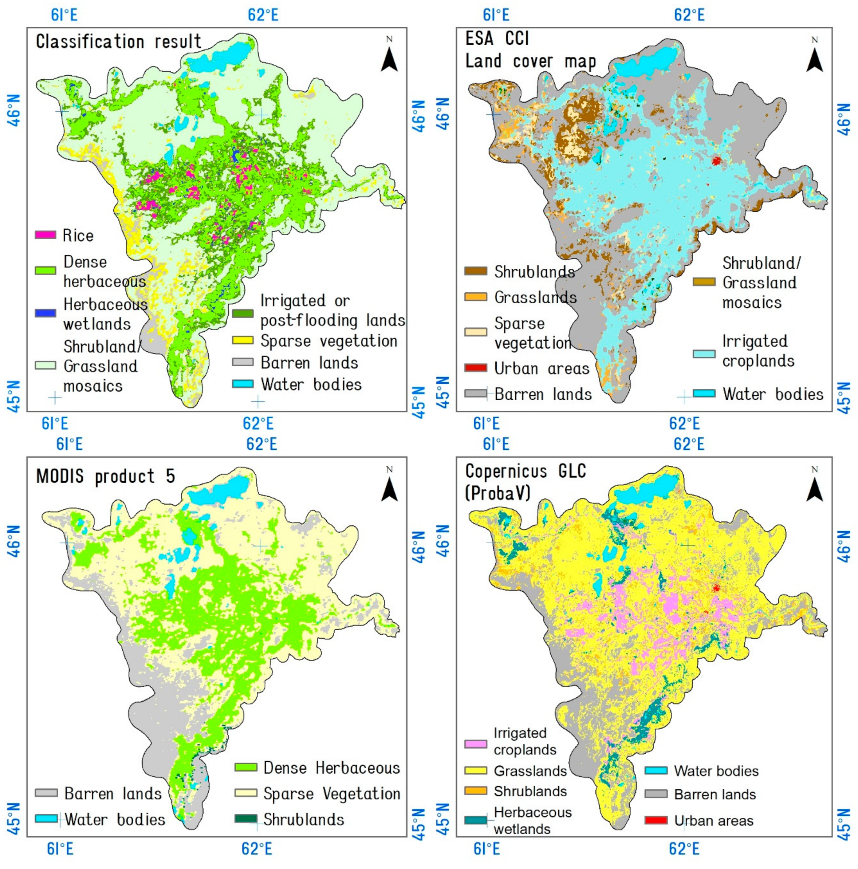
3.3. Area Comparison with Other Land Cover Products

Classification results were compared to three existing land cover products: ESA CCI, MODIS product 5, and Copernicus Global 100 m Land Cover. Data for the year 2015 were selected to compare the same time period. Though classification systems of all products refer to the UN FAO (Food and Agriculture Organization of the United Nations) Land cover classification system [58], several classes and their spatial locations were different due to pixel-based and object-based classification input classes (Figure 11).

We can see that in fact only water bodies and croplands coincide. In the case of our classification results, they are affected by NDVI yearly dynamics and the results are more detailed compared to other products, despite the coarse resolution. Rice croplands in our classification map are distinguished from others. Then, the area comparison of several land cover classes between products was done, which is shown in Figure 12. In the case of croplands, Copernicus GLC (Global Land Cover) product demonstrates the lowest area. The area of the croplands classified during this study integrated three classes: rice croplands, dense herbaceous, and irrigated or post-flooding land cover. These area values were close to the cropland area of ESA CCI map, while the MODIS product 5 had the maximum area for croplands, and the minimum was found on the Copernicus GLC map. Sparse vegetation was low on the ESA CCI map and had a different geographic location, while our study map and MODIS product 5 had close areas, followed by Copernicus GLC. Barren lands were at a minimum in our study map and other maps had different areas, with the maximum seen in the ESA CCI map. Only in the case of the water bodies did MODIS product 5 has the maximum area, followed by our map’s classification results, while two other products demonstrated almost similar results.

The visual classification was another way to check the correspondence of the classification results with satellite remote sensing and ground truth data. In this regard, the NDVI calculated from Landsat on June 14, 2018, along with August 17, 2018, and MODIS NDVI classification results were compared (Figure 13).

As the main efforts in this study were related to forwarded agriculture, the spatial boundary matching of the classified rice croplands and Landsat data were compared. Though the resolution of MODIS was 250 meters, it was found that class boundaries fit Landsat data accurately. The image on June 14, 2018, shows that the highlighted areas have low NDVI, and in the next one, acquired on August 17, 2018, they have the highest NDVI values of up to 0.84. The match of the classes’ boundaries derived from supervised classification and Landsat NDVI was high considering the almost 10-fold difference in spatial resolution.

4. Discussion

The random forests supervised classification machine learning algorithm was used to map land cover, which gave us get good results with an overall accuracy of about 0.8. Statistics on land cover change were calculated and analyzed. The correctness of the obtained classes was checked with Landsat 8 (OLI) images. Detailed land cover maps, including rice cropland, were derived.

Rice croplands had a minimum area in 2004 (~40 km²) and had grown up to 200 km² by 2015, decreased in 2016, and then increased again, demonstrating a growing trend. We also noticed that our results agreed with previous studies on cropland abandonment monitoring [27]. Löw et al. (2018) found that rice production in the Kyzylorda region, which is an administrative region to which the Qazaly irrigation zone belongs, dropped during the period 1993–2002 and increased during 2009–2013. The supervised random forests classification approach let us detect the rice croplands in MODIS images very well. This could be due to their unique phenological features and the irrigation regime, which affected its NDVI pattern. Earlier Jinwei Dong et al. (2015) reported results of the research work devoted to monitoring paddy rice planting in China [59]. They plotted the timeline of the phenological phases of the rice and applied phenology-based algorithms to indicate the paddy rice dynamics using Landsat images. Some of the rice croplands were flooded during our onsite visit, which can be seen on the map from June 14, 2018, where most of the rice croplands had low or negative NDVI because they were covered by water.

Other crop types were not recognized, and we consider several reasons for that. In the case of the alfalfa, the similarity of its seasonal NDVI pattern with the vegetation that was detected as the “dense herbaceous” class could have caused the impossibility of its classification. It was not possible to make classification of the saflor and wheat, since their cropping areas had small spatial dimensions, which were less than the input product’s pixel size of 250 meters, and also because of their undistributed cropping. Therefore, it was not possible to detect them using MODIS images, and perhaps it is better to classify detailed crop maps using satellite remote sensing data with higher spatial resolution. In this regard, we would like to mention that other authors used space images with higher spatial resolution. Teke and Yardimci (2015) used images acquired from Landsat 8 and Hyperion, which have similar spatial resolutions and were able to classify the alfalfa along with the other crop types in Eastern Turkey with 88% and 92% accuracy, respectively [60]. They suggested using a combination of hyperspectral and multispectral images as probably the most effective approach for classification of crops. From the point of view of providing detailed information, it may be the right choice, but at the same time it can be time-consuming, and the approach suggested in our research was appropriate for land cover change monitoring.

The dense herbaceous class demonstrated a constant decrease of 300 km², possibly due to changes in vegetation cover, for example in cases when drying and soil quality affected raising grasses instead of reeds. Their classification was possible because their phenological phases are different from dry area vegetation and shrubs.

The growth of herbaceous wetlands space by 300 km², detected by classification, could be caused by a variety of factors, including changes in the hydrological regime of the Syrdarya river and altering of irrigated, fallow croplands, and the formation of the abandoned agricultural lands. The reeds were observed in most of the observed fallow and abandoned croplands, which could be evidence of elevated groundwater levels. Previously it was reported that some authors used 1-km MODIS images for extraction of the wetland areas [61].

Shrubland/grassland mosaics occupied the largest part of the Qazaly cropland zone in a mostly dry area and had lower NDVI values, which were enough for their classification. Thus, irrigated or post-flooding lands distributed in the surroundings of the flooding zone included mostly hydrophytes, such as the Tamarix and other shrubs, mixed with herbs, which sometimes changed the cultural crops in abandoned croplands.

Sparse herbaceous areas were classified due to having the lowest NDVI values compared to other classes, and they included the abandoned agricultural lands with their poor vegetation.

Water bodies were the local lakes, and the largest ones among them were the Qamystybas, Qotankol, and Shomishkol lakes, among others, which were mostly fed by the Syrdarya river and located on the north part of the study area, and their changes were dependent on the water regime.

Barren lands demonstrated more straight and strong growth, possibly due to the decrease of soil quality and growth of abandoned saline lands, which was observed during fieldwork in 2018.

Though the land cover classification system utilized in this study and the existing MODIS collection 5 product have common classes, the comparison showed large differences in areas, which can be explained by different input classes. For example, field survey results showed that most of the irrigated lands occupied a huge part of the study area. At the same time, an overall decrease in the largest land cover class of the study area was found, which could be evidence of a decrease in agricultural resources.

Using of multitemporal MODIS images of 250-m resolution for land cover classification is an effective approach compared to 500-m, as it lets researchers distinguish different types of vegetation cover, as was earlier reported by Sedano et al. (2005) [62].

In our case, we considered the time period of 2003–2018 due to the availability of remote sensing data from MODIS satellites. However, we could see that the dynamics of the rice croplands corresponded to the main growing trend described by the authors mentioned above. This could be due to economic processes, such as privatization, or some recultivation measures implemented by landowners in the last decade. Other factors, such as population dynamics and employment, and social and economic factors could also have affected land cover change, which could be the baseline for future studies.

The results of this work prove that the approach presented in this paper provides a feasible way to monitor land cover through vegetation dynamics over large areas using MODIS data. The methodology of this research work treats each pixel of the image and proposes accessible data reconstruction and image classification methods, which means it is globally applicable. Furthermore, it lets researchers consider the phenological dynamics of the vegetation cover of the area. The field observation results conducted during this research make it more concrete and raise its accuracy. The supervised classification of terrestrial cover showed comparatively accurate results for rice crops and other classes, which can be observed in the Landsat images. Such results can be used to inventory agricultural land, crop patterns, and environmental studies. Using MODIS images with a coarse resolution of 250 m can be considered as the limitation on one hand, but on the other, it let us cover a huge cropping area and gave us an opportunity to monitor land cover change with high accuracy. As this approach consisted of commonly used methods, it may be considered also for other study areas with similar conditions combined with other remote sensing data of different spatial resolutions. It could contribute to the improvement of the accuracy of classification and monitoring of environmental changes in such arid areas that are experiencing environmental stress. The proposed multitemporal NDVI approach of mapping can be used to create inventory agricultural maps for decision-making purposes, as well as for land cover mapping purposes.

5. Conclusions

This research work aimed to study the spatial and temporal patterns in the land cover of the Qazaly irrigation zone. For this purpose, we have introduced the approach to derive land cover information from the MODIS NDVI with coarse 250-m spatial resolution time series, using a combination of several methods. The initial data consisted of field observation data and Landsat 8 images. They were all processed in three main steps: (1) data preprocessing, (2) supervised classification, and (3) post classification.

Data preprocessing let us prepare the initial data based on inputting ground truth data collected in 2018, calculating NDVI, and true or false color compositions, and MODIS NDVI interpolation together with value filtering and curve fitting. In order to carry out supervised classification, training samples were generated combining ground truth and initial classification values. The core analysis of this research was based on the supervised classification using random forests method. Based on the field survey results (knowing dominant vegetation cover) and using the RF approach, the yearly main land cover patterns were classified for 2003–2018. Results showed that RF classification could accurately detect rice crops but had limited accuracy for other crops.

To evaluate the performance of the RF supervised classification model, yearly confusion matrices of true and predicted land cover classes were created, yet they were not included in this paper. Almost all of the selected land cover classes showed high classification accuracy and featured quite good accuracy metrics. Regarding the approach of a larger part of the sample dataset being generated from the basic classification map, we suggest that future supervised classification research studies pay more attention to collecting more detailed ground truth data. However, in cases where only limited sample data are available, it will still be possible to produce the output land cover classification map, as is shown in this paper.

Although the results of this research show some limitations regarding vegetation classification and sample dataset formation, we believe land cover classification based on phenological patterns of vegetation is still valuable for research studies. The supervised RF classification of the land cover showed comparatively accurate results for rice croplands and other classes, which can be observed in the Landsat images. Such results could be used to inventory agricultural lands, crop patterns, and environmental studies. This approach could be the part of the analysis together with other remote sensing data of coarse and higher spatial resolution to improve the accuracy of the classification and monitoring of environmental changes in such arid areas experiencing ecological stress.

References

1. Tucker, C.J. Red and photographic infrared linear combinations for monitoring vegetation. Remote Sens. Environ. 1979, 8, 127–150. [Google Scholar] [CrossRef] [Green Version]
2. Sellers, P.J.; Dickinson, R.E.; Randall, D.A.; Betts, A.K.; Hall, F.G.; Berry, J.A.; Collatz, G.J.; Denning, A.S.; Mooney, H.A.; Nobre, C.A.; et al. Modeling the Exchanges of Energy, Water, and Carbon Between Continents and the Atmosphere. Science 1997, 275, 502–509. [Google Scholar] [CrossRef] [PubMed] [Green Version]
3. Gouveia, C.; Trigo, R.M.; Dacamara, C.C. Drought and vegetation stress monitoring in Portugal using satellite data. Nat. Hazards Earth Syst. Sci. 2009, 9, 185–195. [Google Scholar] [CrossRef] [Green Version]
4. Sruthi, S.; Aslam, M.M. Agricultural Drought Analysis Using the NDVI and Land Surface Temperature Data; a Case Study of Raichur District. Aquat. Procedia 2015, 4, 1258–1264. [Google Scholar] [CrossRef]
5. Statuto, D.; Cillis, G.; Picuno, P. GIS-based Analysis of Temporal Evolution of Rural Landscape: A Case Study in Southern Italy. Nat. Resour. Res. 2018, 28, 61–75. [Google Scholar] [CrossRef]
6. Hansen, M.C.; DeFries, R.S.; Townshend, J.R.G.; Sohlberg, R. Global land cover classification at 1 km spatial resolution using a classification tree approach. Int. J. Remote Sens. 2000, 21, 1331–1364. [Google Scholar] [CrossRef]
7. DeFries, R.S.; Townshend, J.R.G. NDVI-derived land cover classifications at a global scale. Int. J. Remote Sens. 1994, 15, 3567–3586. [Google Scholar] [CrossRef]
8. Field, C.B.; Potter, C.S.; Randerson, J.T.; Matson, P.A.; Vitousek, P.M.; Mooney, H.A.; Klooster, S.A. Terrestrial ecosystem production: A process model based on global satellite and surface data. Glob. Biogeochem. Cycles 1993, 7, 811–841. [Google Scholar]
9. Townshend, J.R.G.; Justice, C.O.; Kalb, V. Characterization and classification of South American land cover types using satellite data. Int. J. Remote Sens. 1987, 8, 1189–1207. [Google Scholar] [CrossRef]
10. Tucker, C.J.; Townshend, J.R.; Goff, T.E. African Land-Cover Classification Using Satellite Data. Science 1985, 227, 369–375. [Google Scholar] [CrossRef]
11. Stone, T.A.; Schlesinger, P.; Houghton, R.A.; Woodwell, G.M. A map of the vegetation of South America based on satellite imagery. Photogramm. Eng. Remote Sens. 1994, 60, 541–551. [Google Scholar]
12. De Fries, R.S.; Hansen, M.; Townshend, J.R.G.; Sohlberg, R. Global land cover classifications at 8 km spatial resolution: The use of training data derived from Landsat imagery in decision tree classifiers. Int. J. Remote Sens. 1998, 19, 3141–3168. [Google Scholar] [CrossRef]
13. Townshend, J.R.G.; Justice, C.O.; Skole, D.; Malingreau, J.-P.; Cihlar, J.; Teillet, P.; Sadowski, F.; Ruttenberg, S. The 1 km resolution global data set: Needs of the International Geosphere Biosphere Programme. Int. J. Remote Sens. 1994, 15, 3417–3441. [Google Scholar] [CrossRef]
14. Loveland, T.R.; Reed, B.C.; Brown, J.F.; Ohlen, D.O.; Zhu, Z.; Yang, L.; Merchant, J.W. Development of a global land cover characteristics database and IGBP DISCover from 1 km AVHRR data. Int. J. Remote Sens. 2000, 21, 1303–1330. [Google Scholar] [CrossRef]
15. Shao, Y.; Lunetta, R.S.; Ediriwickrema, J.; Iiames, J. Mapping Cropland and Major Crop Types across the Great Lakes Basin using MODIS-NDVI Data. Photogramm. Eng. Remote Sens. 2013, 76, 73–84. [Google Scholar] [CrossRef]
16. Lunetta, R.S.; Knight, J.F.; Ediriwickrema, J.; Lyon, J.G.; Worthy, L.D. Land-cover change detection using multi-temporal MODIS NDVI data. Remote Sens. Environ. 2006, 105, 142–154. [Google Scholar] [CrossRef]
17. Knight, J.F.; Lunetta, R.S.; Ediriwickrema, J.; Khorram, S. Regional Scale Land Cover Characterization Using MODIS-NDVI 250 m Multi-Temporal Imagery: A Phenology-Based Approach. GISci. Remote Sens. 2006, 43, 1–23. [Google Scholar] [CrossRef]
18. Nemani, R.S. Land Cover Characterization Using Multitemporal Red. Ecol. Appl. 1997, 7, 79–90. [Google Scholar] [CrossRef]
19. Wadsworth, P.F.R.; Balzter, H.; Gerard, F.; George, C.; Comber, A. An environmental assessment of land cover and land use change in Central Siberia using quantified conceptual overlaps to reconcile inconsistent data sets. J. Land Use Sci. 2008, 3, 251–264. [Google Scholar] [CrossRef] [Green Version]
20. Kozhoridze, G.; Orlovsky, L.; Orlovsky, N. Monitoring land cover dynamics in the Aral Sea region by remote sensing. SPIE Remote Sens. 2012, 8538, 85381V. [Google Scholar]
21. Wulder, M.A.; White, J.C.; Goward, S.N.; Masek, J.G.; Irons, J.R.; Herold, M.; Cohen, W.B.; Loveland, T.R.; Woodcock, C.E. Landsat continuity: Issues and opportunities for land cover monitoring. Remote Sens. Environ. 2008, 112, 955–969. [Google Scholar] [CrossRef]
22. Homer, C.; Huang, C.; Yang, L.; Wylie, B.; Coan, M. Development of a 2001 National Land-Cover Database for the United States. Photogramm. Eng. Remote Sens. 2004, 70, 829–840. [Google Scholar] [CrossRef]
23. Li, P.; Jiang, L.; Feng, Z. Cross-comparison of vegetation indices derived from landsat-7 enhanced thematic mapper plus (ETM+) and landsat-8 operational land imager (OLI) sensors. Remote Sens. 2013, 6, 310–329. [Google Scholar] [CrossRef]
24. Chen, J.; Chen, J.; Liao, A.; Cao, X.; Chen, L.; Chen, X.; He, C.; Han, G.; Peng, S.; Lu, M.; et al. Global land cover mapping at 30m resolution: A POK-based operational approach. ISPRS J. Photogramm. Remote Sens. 2015, 103, 7–27. [Google Scholar] [CrossRef] [Green Version]
25. Löw, F.; Conrad, C.; Michel, U. Decision fusion and non-parametric classifiers for land use mapping using multi-temporal RapidEye data. ISPRS J. Photogramm. Remote Sens. 2015, 108, 191–204. [Google Scholar] [CrossRef]
26. Gislason, P.O.; Benediktsson, J.A.; Sveinsson, J.R. Random Forests for land cover classification. Pattern Recognit. Lett. 2006, 27, 294–300. [Google Scholar] [CrossRef]
27. Low, F.; Prishchepov, A.V.; Waldner, F.; Dubovyk, O.; Akramkhanov, A.; Biradar, C.; Lamers, J.P.A. Mapping Cropland Abandonment in the Aral Sea Basin with MODIS Time Series. Remote Sens. 2018, 10, 159. [Google Scholar] [CrossRef]
28. Micklin, P. The Aral sea disaster. Annu. Rev. Earth Planet. Sci. 2007, 35, 47–72. [Google Scholar] [CrossRef]
29. Saiko, T.A.; Zonn, I.S. Irrigation expansion and dynamics of desertification in the Circum-Aral region of Central Asia. Appl. Geogr. 2000, 20, 349–367. [Google Scholar] [CrossRef]
30. Saiko, T.S. Geographical and socio-economic dimensions of the Aral Sea crisis and their impact on the potential for community action. J. Arid. Environ. 1998, 39, 225–238. [Google Scholar] [CrossRef]
31. Conrad, C.; Rahmann, M.; Machwitz, M.; Stulina, G.; Paeth, H.; Dech, S. Satellite based calculation of spatially distributed crop water requirements for cotton and wheat cultivation in Fergana Valley, Uzbekistan. Glob. Planet. Chang. 2013, 110, 88–98. [Google Scholar] [CrossRef]
32. Löw, F.; Fliemann, E.; Abdullaev, I.; Conrad, C.; Lamers, J.P.A. Mapping abandoned agricultural land in Kyzyl-Orda, Kazakhstan using satellite remote sensing. Appl. Geogr. 2015, 62, 377–390. [Google Scholar] [CrossRef]
33. Ivushkin, K.; Bartholomeus, H.; Bregt, A.K.; Pulatov, A. Satellite Thermography for Soil Salinity Assessment of Cropped Areas in Uzbekistan. Land Degrad. Dev. 2017, 28, 870–877. [Google Scholar] [CrossRef]
34. Ivushkin, K.; Bartholomeus, H.; Bregt, A.K.; Pulatov, A.; Bui, E.N.; Wilford, J. Soil salinity assessment through satellite thermography for different irrigated and rainfed crops. Int. J. Appl. Earth Obs. Geoinf. 2018, 68, 230–237. [Google Scholar] [CrossRef]
35. Jin, Q.; Wei, J.; Yang, Z.-L.; Lin, P. Irrigation-Induced Environmental Changes around the Aral Sea: An Integrated View from Multiple Satellite Observations. Remote Sens. 2017, 9, 900. [Google Scholar] [CrossRef]
36. Didan, K. MYD13Q1 MODIS/Aqua Vegetation Indices 16-Day L3 Global 250m SIN Grid V006; NASA EOSDIS Land Processes DAAC: Sioux Falls, SD, USA, 2015. [Google Scholar]
37. Huete, A.; Didan, K.; Miura, T.; Rodriguez, E.; Gao, X.; Ferreira, L. Overview of the radiometric and biophysical performance of the MODIS vegetation indices. Remote Sens. Environ. 2002, 83, 195–213. [Google Scholar] [CrossRef]
38. Chen, J.; Jönsson, P.; Tamura, M.; Gu, Z.; Matsushita, B.; Eklundh, L. A simple method for reconstructing a high-quality NDVI time-series data set based on the Savitzky? Golay filter. Remote Sens. Environ. 2004, 91, 332–344. [Google Scholar] [CrossRef]
39. Eckert, S.; Hüsler, F.; Liniger, H.; Hodel, E. Trend analysis of MODIS NDVI time series for detecting land degradation and regeneration in Mongolia. J. Arid. Environ. 2015, 113, 16–28. [Google Scholar] [CrossRef]
40. Pan, Z.; Huang, J.; Zhou, Q.; Wang, L.; Cheng, Y.; Zhang, H.; Blackburn, G.A.; Yan, J.; Liu, J. Mapping crop phenology using NDVI time-series derived from HJ-1 A/B data. Int. J. Appl. Earth Obs. Geoinf. 2015, 34, 188–197. [Google Scholar] [CrossRef]
41. Irons, J.R.; Dwyer, J.L.; Barsi, J.A. The next Landsat satellite: The Landsat Data Continuity Mission. Remote Sens. Environ. 2012, 122, 11–21. [Google Scholar] [CrossRef] [Green Version]
42. OpenStreetMap Contributors. Available online: https://planet.osm.org (accessed on 24 February 2019).
43. NAKZ (National Atlas of Kazakhstan). Environment and Ecology; The Institute of Geography of Kazakhstan: Almaty, Kazakhstan, 2006; Volume 3. (In Russian) [Google Scholar]
44. Eastman, J.R. IDRISI Kilimanjaro: Guide to GIS and Image Processing; Clark University: Worcester, MA, USA, 2003; Volume 1, pp. 87–131. [Google Scholar]
45. Sanli, F.B.; Delen, A. Assessment of vegetation indices for the determination of agricultural crop types. J. Environ. Prot. Ecol. 2018, 19, 417–425. [Google Scholar]
46. Volkova, E.A.; Ogar, N.P.; Rachkovskaya, E.I.; Sadvokasov, P.E.; Hramtsov, V.N. The National Atlas of the Republic of Kazakhstan, map: Vegetation. Almaty 2010, 1, 110–113. [Google Scholar]
47. Eisfelder, C.; Klein, I.; Bekkuliyeva, A.; Kuenzer, C.; Buchroithner, M.F.; Dech, S. Above-ground biomass estimation based on NPP time-series—A novel approach for biomass estimation in semi-arid Kazakhstan. Ecol. Indic. 2017, 72, 13–22. [Google Scholar] [CrossRef]
48. Mousivand, A.; Arsanjani, J.J. Insights on the historical and emerging global land cover changes: The case of ESA-CCI-LC datasets. Appl. Geogr. 2019, 106, 82–92. [Google Scholar] [CrossRef]
49. NGCC. GlobeLand30 Dataset (Provided by National Geomatics Center of China). 2010. Available online: http://www.globeland30.org/GLC30Download/index.aspx (accessed on 31 May 2019).
50. CGLO. Moderate Dynamic Land Cover 100m. Product User Manual (Povided by Copernicus Global Land Operations). 2019. Available online: https://land.copernicus.eu/global/sites/cgls.vito.be/files/products/CGLOPS1_PUM_LC100_V2_I2.10.pdf (accessed on 31 May 2019).
51. Friedl, M.A.; Sulla-Menashe, D.; Tan, B.; Schneider, A.; Ramankutty, N.; Sibley, A.; Huang, X. MODIS Collection 5 global land cover: Algorithm refinements and characterization of new datasets. Remote Sens. Environ. 2010, 114, 168–182. [Google Scholar] [CrossRef]
52. Belgiu, M.; Drăguț, L. Random forest in remote sensing: A review of applications and future directions. ISPRS J. Photogramm. Remote Sens. 2016, 114, 24–31. [Google Scholar] [CrossRef]
53. Breiman, L. Random forests. Mach. Learn. 2001, 45, 5–32. [Google Scholar] [CrossRef]
54. Rodriguez-Galiano, V.F.; Ghimire, B.; Rogan, J.; Olmo, M.C.; Rigol-Sanchez, J.P. An assessment of the effectiveness of a random forest classifier for land-cover classification. ISPRS J. Photogramm. Remote Sens. 2012, 67, 93–104. [Google Scholar] [CrossRef]
55. Cohen, J.A. Coefficient of Agreement for Nominal Scales. Educ. Psychol. Meas. 1960, 20, 37–46. [Google Scholar] [CrossRef]
56. Sasaki, Y. The truth of the F-measure. Teach Tutor Mater. 2007, 1, 1–5. [Google Scholar]
57. Rwanga, S.S.; Ndambuki, J.M. Accuracy Assessment of Land Use/Land Cover Classification Using Remote Sensing and GIS. Int. J. Geosci. 2017, 8, 611–622. [Google Scholar] [CrossRef] [Green Version]
58. Latham, J.; Cumani, R.; Rosati, I.; Bloise, M. Global Land Cover SHARE (GLC-SHARE) Database Beta-Release Version 1.0-2014; Food and Agriculture Organization of the United Nations: Rome, Italy, 2014. [Google Scholar]
59. Dong, J.; Xiao, X.; Kou, W.; Qin, Y.; Zhang, G.; Li, L.; Jin, C.; Zhou, Y.; Wang, J.; Biradar, C.; et al. Tracking the dynamics of paddy rice planting area in 1986–2010 through time series Landsat images and phenology-based algorithms. Remote Sens. Environ. 2015, 160, 99–113. [Google Scholar] [CrossRef]
60. Teke, M.; Yardımcı, Y. Classification of crops using multitemporal hyperion images. In Proceedings of the 2015 Fourth International Conference on Agro-Geoinformatics, Istanbul, Turkey, 20–24 July 2015; pp. 282–287. [Google Scholar]
61. Bansal, S.; Katyal, D.; Garg, J. A novel strategy for wetland area extraction using multispectral MODIS data. Remote Sens. Environ. 2017, 200, 183–205. [Google Scholar] [CrossRef]
62. Sedano, F.; Gong, P.; Ferrao, M. Land cover assessment with MODIS imagery in southern African Miombo ecosystems. Remote Sens. Environ. 2005, 98, 429–441. [Google Scholar] [CrossRef]
Figure 1. Study area map.
Sustainability 11 04035 g001
Figure 2. The workflow of the study.
Sustainability 11 04035 g002
Figure 3. Geometric representation of linear interpolation. Values: (a) before and (b) after interpolation.
Sustainability 11 04035 g003
Figure 4. The Savitzky-Golay filtering example.
Sustainability 11 04035 g004
Figure 5. Initial and smoothed NDVI (Normalized Difference Vegetation Index) time series of different crops (16-day periods between 2003 and 2018).
Sustainability 11 04035 g005
Figure 6. Map of the field observation data (background: Landsat 8 false-color composition, 14/06/2018).
Sustainability 11 04035 g006
Figure 7. Random forests classification sample (adapted from http://dataaspirant.com).
Sustainability 11 04035 g007
Figure 8. The proportion of land cover classes.
Sustainability 11 04035 g008
Figure 9. Changes in land cover classes for 2003–2018.
Sustainability 11 04035 g009
Figure 10. Dynamics of the areas of several land cover classes.
Sustainability 11 04035 g010
Figure 11. Comparison of classification and existing land cover products (2015).
Sustainability 11 04035 g011
Figure 12. Comparison of the classified rice croplands with Landsat-8 NDVI (km2).
Sustainability 11 04035 g012
Figure 13. Comparison of the classified rice croplands with Landsat-8 NDVI.
Sustainability 11 04035 g013