1. Introduction
The El Niño-Southern Oscillation (ENSO) is an irregularly periodical variation in winds and sea surface temperatureswhich arise from the tropical eastern Pacific Ocean andhas climatic effects on a global scale. Consequently, the frequency and strength of extreme weather events driven by the ENSO in China have increased significantly in the past 50 years [
1]. The ENSO is classified into El Niño, La Niña and Neutral, which are the warm, cool, and normal phases of a recurring climate pattern across the tropical and subtropical Pacific, respectively. The systematic disturbances in climate pattern severely affect crop yields and, in turn, affect economic output. The impact measurements of climate variability on agriculture have evolved significantly in recent years (e.g., [
2,
3,
4]). Farmers can adjust their cropping decisions to mitigate the impacts of climate variability and maximize their profits if ENSO information is disseminated in advance. These adjustments to cropping decisions that are driven by ENSO information, such as reallocating planting acreage and altering inputs, are likely to have a positive impact on the variations in economic surplus, which can be explained as the value of an ENSO forecast [
5,
6]. However, the potential of this gain to China’s agricultural sectoris unknown.
In the past decade, the accuracy of China’s climate prediction has been obviously improved. Since 2012, the Beijing Climate Center has progressed with research into a new generation of ENSO monitoring, analysis, and prediction system (SEMAP 2.0) to improve the operational capability of ENSO forecasting. This new system has been applied to real-time operations during its development, but it still faces challenges in how accurately it can predict the intensity, occurrence, and phase transition time of the ENSO. For example, the forecast period shows a large degree of dispersion after less than one season for different forecasting patterns. Measuring the value of ENSO forecasting to China’s agricultural sector, at different levels of forecast accuracy, will provide evidence to support investment in the development of an ENSO forecast system.
This study is the first to evaluate the value of ENSO forecasting at different levels of accuracy to China’s agricultural sector. The measurement has two steps: (1) estimating yield effects under different ENSO phases and (2) translating the yield effects into economic effects considering realistic market conditions. Regarding the first step, existing research mostly applies biophysical simulation models to estimate the differences between crop yields during ENSO phases. The present study, however, uses an econometric approach to identify the impacts of ENSO on crop yields [
7]. Specifically, we apply the Weibull distribution to model crop yields under different ENSO phases, which was proven to be more appropriate for explaining the variation in crop yields due to extreme events [
8]. Under the framework of Bayesian decision theory, the second step pioneers the application of China’s Agricultural Sector Model (CASM) (Yi et al. (2018) discussed CASM in detail.) to translate the impact of the ENSO on crop yields into economic effects.
The results show that the ENSO has noticeable and heterogeneous effects on crop yields over the selected crops by regions in China. ENSO forecasting allows farmers to adjust their cropping decisions and consequently, contributes to economic surplus. In addition, the value of ENSO forecast information ranges from CNY 167 to 3168 million with improved forecasting accuracy. This study inquires whether an investment in ENSO forecasting would be cost-effective in China and has critical implications for improving China’s ENSO forecast system.
2. Materials and Methods
2.1. ENSO Effects on Crop Yields
Compared to other climatic phenomena, the ENSO has the greatest potential to impact crop yields. Modeling of yield distributions draws much attention in the literature on crop insurance and agricultural risk management. The method used for measuring the impacts of ENSO phases on crop yields is based on literature that focuses on agricultural insurance ratings [
8,
9,
10,
11]. The concept is to construct a series of comparable yields over time from historical yield observations [
9]. The impact measurement of ENSO phases on crop yields involves three steps: (1) normalization of crop yields, (2) categorization of ENSO years, and (3) modeling of crop yield distribution.
2.1.1. Crop Yield Normalization
Considering the availability of yield data, county-level data has been collected from 1981 to 2014 for the five major crops in China, namely rice, wheat, maize, soybean, and cotton, which were obtained from the Agricultural Information Institute of the Chinese Academy of Agricultural Science. The five selected crops accounted for over 60% of planting areas in 2014 (China Statistical Yearbook 2017). We first detrend the yields for the five crops in 365 prefecture-level cities to eliminate additional influences over crop production, such as time trends and technological advancements. The yields are assumed to follow a second-order polynomial trend. For a specific prefecture-level city which includes several counties, a crop yield in county
is determined by:
where
is the yield for county
at time
(
= 1981, …, 2014), and
is the error term. We also add a county dummy variable
to remove regional heterogeneity in each of counties.
The predicted yield (
) and deviation from the predicted yield (
) are obtained from Equation (1). Goodwin et al. (1998, 2004) [
9,
12] indicated that deviation from the time trend tends to be proportional to the yield level. We have normalized all yields to 2014 equivalents as follows:
where
represents the normalized yields from 1981 to 2014 for county
.
denotes the normalized yield of a given prefecture-level city based on the average values of county-level yield in county
over
counties in the city.
2.1.2. ENSO Phase Categorization
ENSO phases (El Niño and La Niña) are determined based on a three-month running mean ofsea-surfacetemperature anomalies (SSTA) in the Niño 3.4 region (170° W–120° W, 5° S–5° N) proposed by the National Oceanic and Atmospheric Administration (NOAA) (Silver Spring, MD, USA). If the index exceeds 0.5 °C for five consecutive months, then the year is classified as being in the El Niño phase. If the index falls below −0.5 °C for five consecutive months, then the year is classified as being in the La Niña phase. All other years are defined as the neutral phase.
Table 1 lists the ENSO historical events from 1981 and 2014.
We divide the years from 1981 to 2014 into three phases (El Niño, La Niña, and neutral), and the remaining periods excluded from
Table 1 are defined asthe neutral phase. If an El Niño event happened in the period from sowing to harvesting a crop, then we categorize that crop year as being in the El Niño phase. La Niña years are defined similarly to El Niño, and the remaining periods are classified as the neutral phase for the crop. The sowing and harvesting time vary among different crops across regions, and the ENSO phase categorizations for each crop across regions are shown in detail in
Appendix A.
2.1.3. Modeling Crop Yield Distribution
To compare the effects on crop yields, we model the yield distribution to estimate the expected crop yields under different ENSO phases. Popular parametric and nonparametric methods are used for modeling crop yields, such as beta distribution [
13], gamma distribution [
14], Weibull distribution [
8], and standard nonparametric kernel method [
15]. We chose the Weibull distribution to model the crop yields because of the method’s flexibility and simplicity; Chen et al. (2004) [
8] demonstrated that the Weibull distribution is suitable for explaining the crop yield density in frequent extreme events. The density function of a simplified Weibull random yield is shown as follows:
where
is theshape parameter (
), and
is thescale parameter (
). Subscript
denotes various ENSO phases (El Niño, La Niña, and neutral).
is the normalized yield at phase
. Parameters (The parameter estimators are available upon request.)
and
can be estimated using the maximum likelihood estimation method. The log-likelihood function (
L) is shown in the Equation (5).
Then we calculate themeanof a Weibullrandom variable from Equation (6), so the mean yield can be obtained.
where
is the gamma function.
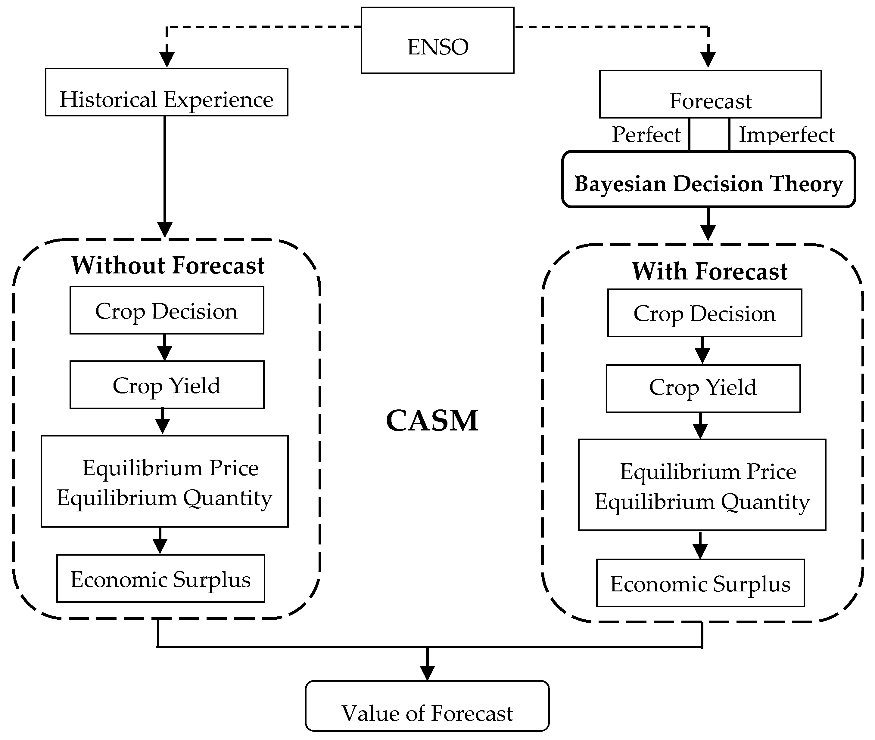
2.2. Conceptual Framework
This section describes the framework used to evaluate ENSO forecasting. In the absence of ENSO forecasts, farmers make cropping decisions according to their historical experience. However, with ENSO forecast information available, farmers are expected to adjust their cropping behaviors to maximize their profits in agriculture [
5,
16]. Changes to cropping decisions are likely to affect the supply of agricultural products, which further influences the quantity and possibly affects the market commodity price due to China’s position of strength in the agricultural trade’s global market. The shift in market equilibrium ultimately affects economic surplus, including that of consumers and producers.
Appendix B describes the shift in supply curves and market equilibrium. The outer aggregation forms its expectation as a convex combination of all possible economic surplus under different ENSO phases weighted by their respective probabilities. The value of ENSO information is defined as the difference between the expected economic surplus obtained with and without forecast information. Note that the study assumes that farmers react to ENSO forecasts by modifying the planting acreage of their crops. Other adjustments, such as irrigation, labor, crop varieties, and calendar, are assumed to be fixed in each region. The value of ENSO information presented here does not include benefits that could occur due to other adjustments, except the responses in crop mix, which are likely to be positively affected by the development of the ENSO prediction system.
Figure 1 shows the conceptual analysis framework, and the formalization is outlined in the following section.
2.2.1. Decision Making without ENSO Forecasts
We begin by examining the scenario without ENSO forecasting. Let the random variable
denote ENSO phases (E = El Niño, L = La Niña, N = neutral). The optimal cropping pattern remains in the long run, given various yields under the realized state of ENSO from the above theoretical conclusion. For a particular ENSO phase
, the shift in market supply due to yield change in each region for each crop can be captured by CASM. Thus, the economic surplus—including consumer and producer surplus—based on the aggregate market demand and supply curves can be estimated. In practice, the expected total economic surplus is given as:
where
is a realization of ENSO phase
,
denotes the economic surplus given the realized ENSO phase
, and
is the probability when
, which can be calculated by the frequency of each ENSO phase.
2.2.2. Decision Making with ENSO Forecasts
If ENSO phase forecast information is disseminated before the planting season, then farmers can adjust their cropping decisions using Bayesian decision theory. Let random variable
denote the forecasted ENSO phase, whereas
is a realization of
. The values of
are the same as
(E = El Niño, L = La Niña, N = neutral). Given the forecasted ENSO phase
, a farmer uses this information to update the prior probability
according to Bayesian decision theory.
where
,
is the posterior probability, and
is forecast skill.
As a result of ENSO phase forecasting, farmers adjust their cropping patterns to achieve maximum benefit. Farmers’ decision making relies on historical experience and forecast information. The optimal cropping pattern and economic surplus depend on achieving both forecasted and realized phases. In practice, the expected economic surplus is calculated by averaging the conditional economic surplus over the probability of
to:
where
, which denotes the conditional expected economic surplus given
. Note that farmers account for the possibility of incorrect phase forecast by averaging over
.
According to the above analysis, the value of ENSO phase forecast is given by:
The value of ENSO forecasting in a particular year is not necessarily positive because a biased forecast may result in a loss of economic surplus. However, the value of using forecast information contributes to the long-term increase ineconomic surplus.
2.2.3. China’s Agricultural Sector Model
We apply China’s Agricultural Sector Model (CASM) to translate the yield effects of ENSO to economic effects. This model simulates an economic equilibrium by maximizing farmers’ profits and minimizing consumers’ costs. The approach is motivated by Samuelson (1952) [
17], who suggested solving optimization problems whose first-order conditions constituted a system of equations characterizing a market equilibrium. Underlying this mechanism is the First Fundamental Theorem of Welfare Economics, which dictates that an allocation of resources that maximizes producers’ profits, consumers’ utility, and clears all markets, is Pareto Optimal (PO). CASM is structured based on the PO theory.
CASM is a multiple-commodity, price endogenous, partial equilibrium model applied to estimate the value of ENSO forecasting. This bottom-up, mathematical programming model represents the monthly production of primary agricultural products over growing seasons across China, reflecting national markets and regional resources plus socioeconomic constraints as discussed in McCarl and Spreen (1980) [
18]. CASM is used to reflect national agricultural product markets under regional resource constraints, such as land and labor. Yi et al. (2018) [
19,
20] discussed the basic structure of the model (see
Appendix C). CASM features 365 prefecture-level cities as sub-regions. Each sub-region possesses different resources in terms of available arable land and labor, along with varying cropping and livestock mixes with different production budgets across China. Cropping patterns in each sub-region are portrayed by representative farm models. These models mimic the technical and economic environment of producers in each sub-region, as discussed in Adams et al. (1986) [
21]. The objective function of the model is to maximize the area under the demand curves ratherthan the area under the supply curves, which is introduced in
Appendix B.
CASM provides an aggregated representation of China’s agricultural sector and needs to be structured to adequately represent that sector. We formed the model (as discussed above) and calibrated it to match observed production and consumption data. We employed the positive mathematical programming approach developed by Howitt (1995) [
22] that manipulates the form of the production costs in an effort to replicate observed cropping patterns and livestock numbers. A classic quadratic form wasused to calibrate against the observed production levels. The CASM model was calibrated against 2014 observations due to data availability. In current research [
19,
20], CASM results on commodity production and prices closely matched the observed data. The crop and livestock prices and quantities werewithin 5% of the actual observations (see
Appendix D). Thus, CASM is suitable for further analysis.
2.2.4. Information Sources for CASM Specification
Sixteen primary field crops and six types of livestock are produced regionally in CASM when local conditions allow. The regional crop and livestock production budgets, as well as farm gate prices, were obtained from data compiled by China Agricultural Product Cost and Revenue (2015). Agricultural commodity trade data werefrom the USDA. Data on crop planting and harvesting time wereobtained from the USDA report on Major World Crop Areas and Climatic Profiles (It is available at
https://www.usda.gov/oce/weather/pubs/Other/MWCACP/.) and agronomists’ suggestions, if needed. The storage costs for major commodities werefrom Chen (2007) [
23]. The elasticitiesof labor supply werefrom Feng and Zhang (2012) [
24] and wereassumed to be equal across all regions. The demand elasticity data for primary products wereadopted from Zhang (2004) [
25]. All prices weredeflated to 2000 levels.
We categorized observed years to one of three ENSO phases based on the index derived by observed SSTA proposed by NOAA. The years in each category correspond to the first three months of the ENSO year namely October, November, and December from the definition of the Center for Ocean-Atmospheric Prediction Studies (It is available at
https://www.coaps.fsu.edu/jma.). The ENSO phase categorization from 1981 to 2014 is listed in
Table 2. We assumedthe frequencies of each ENSO phase remain constant in the future. The frequencies of each ENSO phase
wereset to
,
, and
that are shown in
Table 2.
Considerable uncertainty exists in ENSO forecasting [
15,
26], particularly the so-called “spring predictability barrier” that hinders accurate ENSO forecasting [
27,
28,
29,
30] and may lead to mistakes in decision making [
26]. To reflect this reality, four hypothetical levels of forecast skills—namelyperfect, high, moderate, and low—wereconsidered to measure the value of ENSO forecast information. The forecasting accuracies of perfect, high, moderate, and low wereset to 100%, 90%, 70%, and 50%, respectively, and the details are listed in
Table 3. According to Equation (8), we obtained the corresponding posterior probabilities in
Table 4.
3. Results and Discussion
3.1. Effects of ENSO on Yields
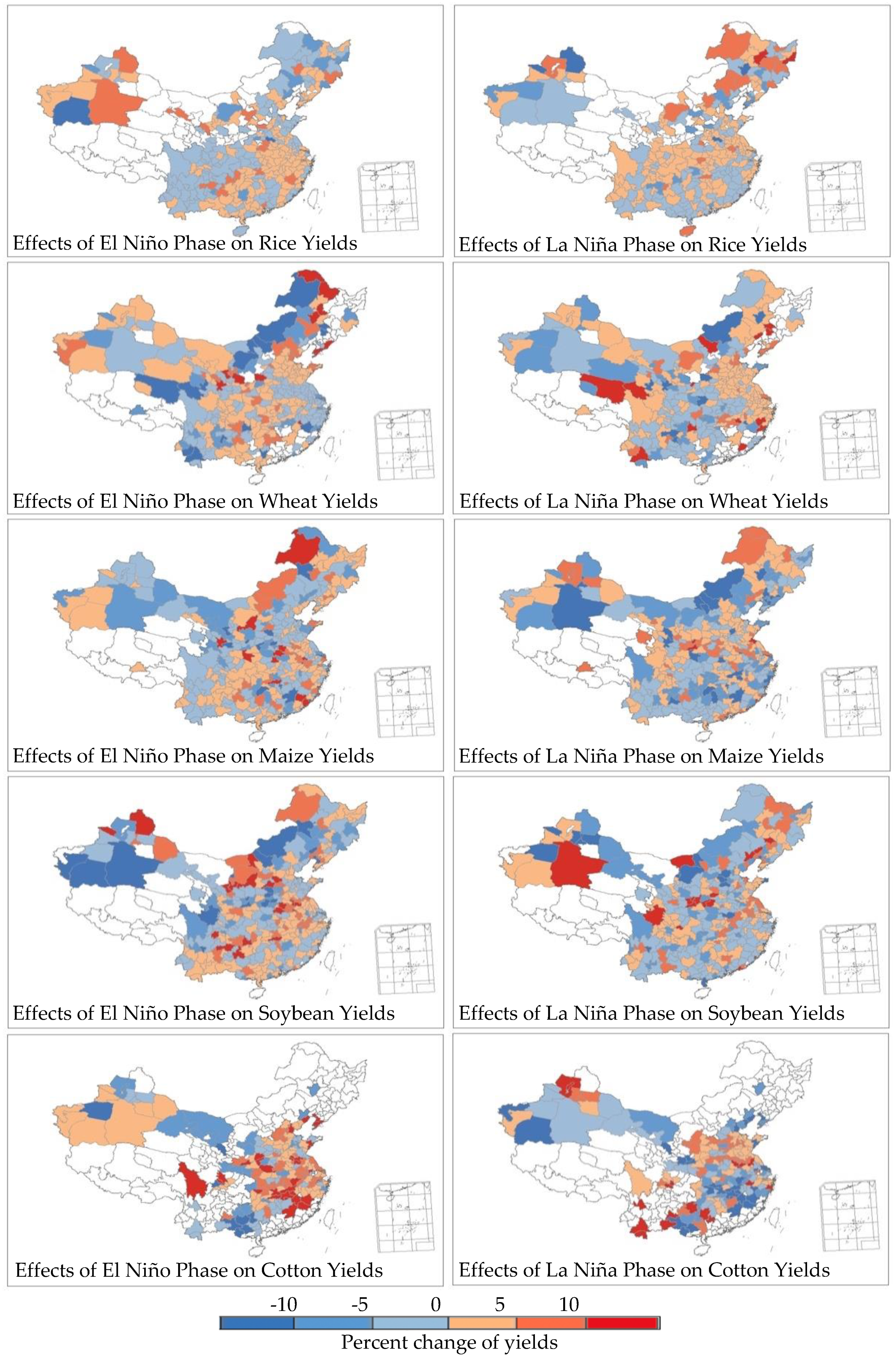
This study first presents the effects of ENSO on crop yields across prefecture-level cities in China.
Figure 2 illustrates the yield effects from El Niño and La Niña phases. The percent change in yield for each ENSO phase is defined as the deviation from average yield, which is computed by the weighted average over all the three ENSO phases. The weights are computed based on the historical frequency of each ENSO phase. According to the frequencies of ENSO phases in
Appendix A, for example, the weights of wheat in Heilongjiang, Jilin, and Liaoning are 0.470, 0.265, and 0.265 for El Niño, La Niña, and neutral phases, respectively. We calculate the percent change using average yields because farmers normally make decisions based on historical data.
Figure 2 shows the heterogeneous yield effects from the ENSO over the selected crops across regions. The ENSO leading signals are not uniform within a single province, and the crop yield responses are regionalized [
31]. Crop yield responses to ENSO phases reverse in different regions, which could be ascribed to conditions offered by varying agriculture facilities. Shuai et al. (2013) [
31] indicated that the responses of crop yields to ENSO phases in western China reversed their sign before 1980 and after 1980 because of improvements made to agriculture facilities, the most significant of which is probably irrigation conditions [
32,
33,
34,
35]. Over all, the ENSO has less of an impact on rice yields to that of other crops, and the yields are more sensitive to the ENSO at high latitudes. Cotton yields are most sensitive to the ENSO and demonstrate over 10% yield changes in most regions.
Generally, the yield effects in El Niño and La Niña phases over the selected crops in the same region, especially in the main crop planting area, are opposite. For example, the yield effects of El Niño and La Niña phases on rice yields are approximately reversed in northeast China. Moreover, the yield effects of El Niño and La Niña phases on wheat yields are evidently reversed in the North China Plain. Similarly, the yield effects of El Niño and La Niña on maize are generally opposite in the Huang–Huai–Hai region and the two ENSO phases affect soybean yields in China’s three northeastern provinces (Heilongjiang, Jilin, and Liaoning) in reverse. In addition, El Niño and La Niña phases affect cotton yields in opposite directions across most production regions.
Overall, these heterogeneous effects provide a basis for the economic analysis of ENSO forecasting, and we can place this percentage change information into CASM to test whether crop mix adaptation during the different ENSO phases generates a benefit to China’s agriculture sector.
3.2. ENSO Forecast Value
Using the economic results obtained from CASM as a basis, we can acquire the ENSO forecast values at different levels of prediction accuracy. The results indicate that the agricultural sector will benefit from ENSO forecasting (see
Table 5). The total economic surplus with ENSO forecasting is significantly larger than it is without ENSO forecasting, and the information value is generally positive, although these gains decrease accordingly in response to reduced forecast accuracy. The value of perfect ENSO phase forecasting is CNY 3168 million, while the information value sharply falls to CNY 167 million at the lower level of forecast accuracy, which accounts for only 5% of that under perfect forecast. The results warn that only accurate ENSO information is helpful for farmers, not poor forecasting.
The changes in ENSO forecasting precision also redistribute the economic surplus between consumers and producers.
Table 5 shows that producers always benefit from ENSO forecasting, and the gain increases with improved accuracy. The direction of the shift in consumer surplus varies with forecast precision. Consumers suffer from ENSO forecasting when the level of forecast accuracy is perfect or high. When the precision drops to a moderate level, consumers benefit, however, consumer surplusagain decreases if the ENSO forecast accuracy falls to 50%. The variation in consumer surplus is not necessarily monotonic, which can be explained as follows.
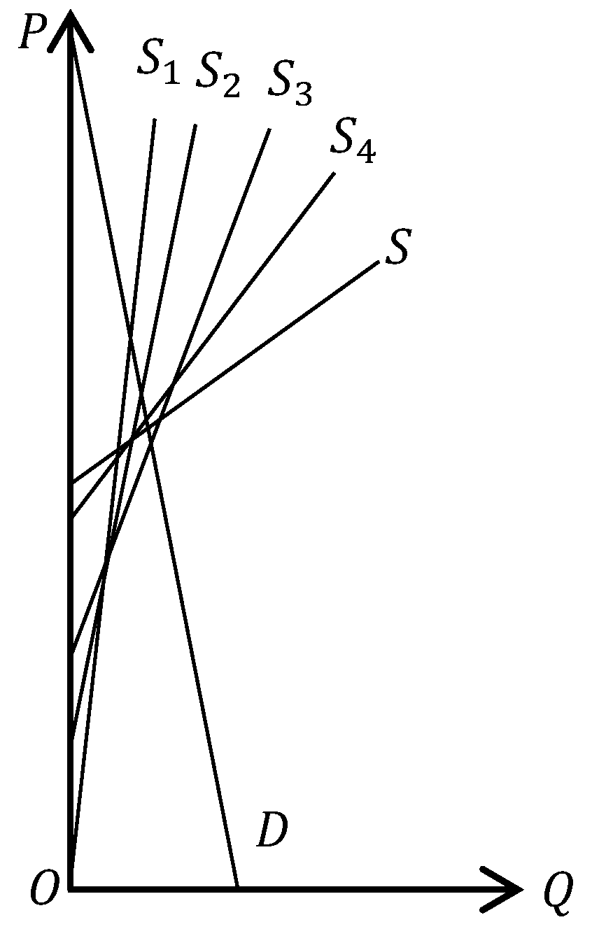
The changes in consumer and producer surplus are attributed to the shift in the aggregate market supply curve across all agricultural products. Note that the intercept and slope of the aggregate market supply curve change simultaneously due to the shift in the supply curve for each agricultural product with the reallocation of crops’ planting acreage under different ENSO forecast accuracies.
Figure 3 presents the possible cases by shifting the aggregate market supply curve under alternative ENSO prediction precision according to the results in
Table 5.
denotes the aggregate market supply curve of an agricultural product without ENSO forecast.
,
,
, and
denote aggregate market supply curves under perfect, high, moderate, and low accuracy of ENSO forecast, respectively. Note that the supply of an agricultural product is computed by the average over all the three ENSO phases, which can be referred to the calculation of expected economic surplus in
Section 3.
denotes the aggregate market demand curve of an agricultural product.
Figure 3 shows the increase in the intercept and the decrease in the slope of the supply curve with the reduction in ENSO forecast accuracy. The decrease in the slope of the supply curve implies the increase in the sensitivity of agricultural supply market with the decreasing ENSO forecast information. In particular, the farmers are more likely to produce short-cycle, storable agricultural products with greater price elasticity of supply when less information is available. A sharp change in the slope of the supply curve exists when the ENSO forecast accuracy drops from high to moderate level. As a result, the variation in consumer surplus changes from a decreasing to an increasing trend, whereas the total economic surplus keeps falling. When the forecast precision falls to a low level, the sharp increase in the intercept of the supply curve will reverse the upward trend of consumer surplus. The losses in consumer surplus under the perfect, high, and low accuracies of ENSO forecasting result from the increase in the agricultural product prices; conversely the reduction in prices under the moderate accuracy of forecast brings potential gain to consumers.The detailed analysis ofthe consumer and producer surplus can be referred to in
Appendix B.
Our estimates are comparable with studies conducted by other countries. Solow et al. (1998) evaluated the expected economic value of perfect ENSO forecasting for US agriculture as being equal to $498 million (The expected economic value of perfect ENSO forecast for U.S. agriculture was 323 million measured in 1995 dollars and deflated to 2014 dollars here.) (CNY 3059 million). Adams et al. (2003) found that a perfect ENSO early warning system generated $87 million (The benefit of a perfect ENSO early warningsystem for Mexican agriculture was 47.4 million in 2000 dollars and deflated to 2014 dollars here.) (CNY 534 million) benefit for Mexican agriculture. Therefore, the total ENSO forecast value for China’s agriculture, at perfect accuracy level (CNY 3168 million) is greater than the ENSO forecast value for other countries. However, the value of perfect ENSO information for China’s agriculture is relatively small when considering the nation’s gross agricultural output (CNY 5477 billion). This finding implies that the ENSO impacts on Chinese agriculture are less serious than they are in the US.
3.3. Effects of ENSO Forecast on Crop Production
Considering that farmers adopt the ENSO forecast to redistribute the land allocated to different crops, which influences production, the gross production for each crop is not guaranteed to increase under alternative forecast accuracy. Under the serious food security concerns held by China’s central government, we analyze the variation of crop production if ENSO forecasting is available.
Table 6 presents the results of planted area changes for each crop with ENSO forecast compared with the scenario without ENSO forecast calculated by totaling the changes over regions. Under different predicted ENSO phases, farmers alter the hectares planted for each crop combined with the prediction precision. We find that farmers increase the amount of land devoted to wheat and cotton when anEl Niñophase is predicted under all forecast accuracy. If aLa Niña phase is predicted, then farmers decrease the planting acreage for all crops under perfect ENSO forecast and gradually increase soybean and cotton acreage when the forecast accuracy reduces. Less land is used in maize, soybean, and cotton planting when the neutral phase is predicted. Moreover, the planting areas of these crops increase as ENSO prediction skill improves within a prefecture-level city (The results are available upon request.), which implies accurate ENSO information stimulating farmers to adjust cropping patterns.
We further estimate the variation of crop production when ENSO forecast is available, and the framework is similar to the calculation of expected economic surplus in
Section 3 (see
Appendix E). The results of changes in crop production are given in
Table 7. The changes in crop production with ENSO forecast in the long run compared with the gross production in China are small, which is consistent with the result from Chen et al. (2000) [
36]. Because the ENSO information is considered at a national level, the increase in crop production in some prefecture-level cities might be counteracted by the reductions in others. Specifically, the ENSO forecast leads to positive influences on rice and cotton production and negative impacts on soybean production. For wheat and maize, the ENSO forecast positively affects their production when the forecast accuracy is over 50%, however, negatively affects their production when the forecast accuracy falls to 50%.
Comparing the results in
Table 6 and
Table 7, the decreases in crop planting acreage seems to conversely to contribute to crop production, which can be ascribed to the differences in yields across regions. The small increases in planting acreage in high-yield regions and big decreases in planting acreage for low-yield regions will lead to a national reduction inplanting acreage and simultaneously an increase in production. For example, the small increases in maize planting acreage in Jilin, Heilongjiang, and Inner Mongolia in apredicted El Niño phase will offset decreases in maize production due to the large reductions in planting acreage in Henan and Shaanxi (The changes in planting acreage and production of the five selected crops with ENSO forecast at provincial level are available upon request.). The results indicate that ENSO information can help farmers to make optimal panting decisions that maximize profit. Soybean is a crop that is adversely affected by ENSO forecasting and thereductions in production are minor under different ENSO forecasting accuracies. Therefore, ENSO forecasting conclusively does not harm the food supply in China.
4. Conclusions
This research shows that ENSO, under different phases, has noticeable and heterogeneous effects on crop yields over selected crops across prefecture-level cities in China. ENSO forecasting is useful for the adjustment of farmers’ cropping decisions, which leads to a shift in the supply of agricultural products andultimately, a benefit in the form of an economic surplus, which is, in turn, defined as the value of ENSO forecast. This research first confirms that ENSO forecasting has significant economic value to China’s agricultural sector. The value of ENSO forecasting ranges from CNY 167 to 3168 million depending on the accuracy of the forecast, providing a justification for investment in developing ENSO forecasting systems. The considerable returns offered by ENSO forecasting are likely to have an implication for China’s investments in agricultural meteorology.
Our findings are supported by the method improvement of the Weibull distribution yield model. We first normalized the yield data by removing time trends and regional heterogeneity, then applied Weibull distribution to model the normalized crop yields under alternative ENSO phases, a model that is proven the best to explain the variation of crop yields by Chen et al. (2004) [
8]. In addition, the study pioneered the application of CASM considering commodity price responses in the market to translate the yield effects resulting from ENSO into economic effects under the framework of Bayesian decision theory.
In light of existing research, this study has some limitations that tend to underestimate the value of ENSO forecasting to agriculture. First, we only considered the yield effects ofthe ENSO for five selected crops due to the availability of data. If more crops were considered in our model, the value of ENSO forecasting to China’s agriculture sector would probably be greater. Second, we assumed that farmers react to ENSO forecasts by modifying the planting acreage of their crops. Other adjustments, such as irrigation, labor, crop varieties, and calendar, were assumed to be fixed in each region. However, these additional factors need to be considered in future research.
Author Contributions
Conceptualization, Y.L. and F.Y.; Data curation, Y.L. and Y.W.; Formal analysis, Y.L.; Funding acquisition, Y.L. and F.Y.; Investigation, Y.L., F.Y. and Y.W.; Methodology, Y.L. and F.Y.; Project administration, F.Y.; Resources, Y.L. and F.Y.; Software, Y.L. and F.Y.; Supervision, F.Y.; Validation, Y.L.; Visualization, Y.L.; Writing—original draft, Y.L.; Writing—review andediting, Y.L., F.Y. and R.G.; Y.L.and F.Y. share the senior authorship.
Funding
This research was funded by the National Natural Science Foundation of China, grant number 71673137; Nanjing Agricultural University, grant number SKTS2017001; Postgraduate Research & Practice Innovation Program of Jiangsu Province, grant number KYCX18_0708.
Acknowledgments
Authors gratefully acknowledge the financial support by the Priority Academic Program Development of Jiangsu Higher Education Institutions (PAPD), the China Center for Food Security Studies at Nanjing Agricultural University, the Jiangsu Rural Development and Land Policy Research Institute, the Jiangsu Agriculture Modernization Decision Consulting Center, and the Jiangsu Provincial Department of Education.
Conflicts of Interest
The authors declare no conflict of interest.
Appendix A
Table A1.
ENSO phase categorization for rice, 1981–2014.
Table A1.
ENSO phase categorization for rice, 1981–2014.
| Region | Neutral | El Niño | La Niña |
|---|
| Whole Region | 1981 | 1982 | 1985 |
| 1984 | 1983 | 1988 |
| 1989 | 1986 | 1995 |
| 1990 | 1987 | 1998 |
| 1993 | 1991 | 1999 |
| 1996 | 1992 | 2000 |
| 2001 | 1994 | 2007 |
| 2003 | 1997 | 2010 |
| 2005 | 2002 | 2011 |
| 2008 | 2004 | |
| 2012 | 2006 | |
| 2013 | 2009 | |
| 2014 | | |
Table A2.
ENSO phase categorization for wheat, 1981–2014.
Table A2.
ENSO phase categorization for wheat, 1981–2014.
| Region | Neutral | El Niño | La Niña |
|---|
| Heilongjiang, Jilin, Liaoning | 1981 | 1982 | 1985 |
| 1984 | 1983 | 1988 |
| 1986 | 1987 | 1989 |
| 1990 | 1991 | 1998 |
| 1993 | 1992 | 1999 |
| 1994 | 1997 | 2000 |
| 1995 | 2002 | 2008 |
| 1996 | 2004 | 2010 |
| 2001 | 2009 | 2011 |
| 2003 | | |
| 2005 | | |
| 2006 | | |
| 2007 | | |
| 2012 | | |
| 2013 | | |
| 2014 | | |
| Fujian, Guangdong, Guangxi, Hainan, Chongqing, Guizhou, Sichuan, Tibet, Yunnan, Henan, Hubei, Hunan, Anhui, Jiangxi, Shanghai, Zhejiang, Jiangsu | 1981 | 1982 | 1985 |
| 1984 | 1983 | 1989 |
| 1986 | 1987 | 1996 |
| 1990 | 1988 | 1999 |
| 1991 | 1992 | 2000 |
| 1993 | 1995 | 2001 |
| 1994 | 1997 | 2008 |
| 2002 | 1998 | 2011 |
| 2004 | 2003 | 2012 |
| 2006 | 2005 | |
| 2009 | 2007 | |
| 2013 | 2010 | |
| 2014 | | |
| Beijing, Hebei, Tianjin, Inner Mongolia, Gansu, Ningxia, Qinghai, Shaanxi, Shanxi, Shandong, Xinjiang | 1981 | 1983 | 1985 |
| 1982 | 1988 | 1989 |
| 1984 | 1992 | 1996 |
| 1986 | 1995 | 1999 |
| 1987 | 1997 | 2000 |
| 1990 | 1998 | 2001 |
| 1991 | 2003 | 2008 |
| 1993 | 2005 | 2011 |
| 1994 | 2007 | 2012 |
| 2002 | 2010 | |
| 2004 | | |
| 2006 | | |
| 2009 | | |
| 2012 | | |
| 2014 | | |
Table A3.
ENSO phase categorization for maize, 1981–2014.
Table A3.
ENSO phase categorization for maize, 1981–2014.
| Region | Neutral | El Niño | La Niña |
|---|
| Heilongjiang, Jilin, Liaoning | 1981 | 1982 | 1985 |
| 1984 | 1983 | 1988 |
| 1989 | 1986 | 1995 |
| 1990 | 1987 | 1998 |
| 1993 | 1991 | 1999 |
| 1996 | 1992 | 2000 |
| 2001 | 1994 | 2007 |
| 2003 | 1997 | 2010 |
| 2005 | 2002 | 2011 |
| 2008 | 2004 | |
| 2012 | 2006 | |
| 2013 | 2009 | |
| 2014 | | |
| Fujian, Guangdong, Guangxi, Hainan, Beijing, Hebei, Tianjin, Inner Mongolia, Gansu, Ningxia, Qinghai, Shaanxi, Shanxi, Shandong, Xinjiang | 1981 | 1982 | 1985 |
| 1984 | 1983 | 1988 |
| 1989 | 1986 | 1998 |
| 1990 | 1987 | 1999 |
| 1993 | 1991 | 2000 |
| 1994 | 1992 | 2007 |
| 1995 | 1997 | 2010 |
| 1996 | 2002 | 2011 |
| 2001 | 2004 | |
| 2003 | 2006 | |
| 2005 | 2009 | |
| 2008 | | |
| 2012 | | |
| 2013 | | |
| 2014 | | |
| Chongqing, Guizhou, Sichuan, Tibet, Yunnan, Henan, Hubei, Hunan, Anhui, Jiangxi, Shanghai, Zhejiang, Jiangsu | 1981 | 1982 | 1988 |
| 1983 | 1986 | 1995 |
| 1984 | 1987 | 1998 |
| 1985 | 1991 | 1999 |
| 1989 | 1994 | 2007 |
| 1990 | 1997 | 2010 |
| 1992 | 2002 | 2011 |
| 1993 | 2004 | |
| 1996 | 2006 | |
| 2000 | 2009 | |
| 2001 | | |
| 2003 | | |
| 2005 | | |
| 2008 | | |
| 2012 | | |
| 2013 | | |
| 2014 | | |
Table A4.
ENSO phase categorization for soybean, 1981–2014.
Table A4.
ENSO phase categorization for soybean, 1981–2014.
| Region | Neutral | El Niño | La Niña |
|---|
| Whole Region | 1981 | 1982 | 1988 |
| 1983 | 1986 | 1998 |
| 1984 | 1987 | 1999 |
| 1985 | 1991 | 2007 |
| 1989 | 1997 | 2010 |
| 1990 | 2001 | 2011 |
| 1992 | 2004 | |
| 1993 | 2006 | |
| 1994 | 2009 | |
| 1995 | | |
| 1996 | | |
| 2000 | | |
| 2001 | | |
| 2003 | | |
| 2005 | | |
| 2008 | | |
| 2012 | | |
| 2013 | | |
| 2014 | | |
Table A5.
ENSO phase categorization for cotton, 1981–2014.
Table A5.
ENSO phase categorization for cotton, 1981–2014.
| Region | Neutral | El Niño | La Niña |
|---|
| Henan, Hubei, Hunan | 1981 | 1982 | 1985 |
| 1984 | 1983 | 1988 |
| 1990 | 1986 | 1989 |
| 1993 | 1987 | 1998 |
| 1994 | 1991 | 1999 |
| 1995 | 1992 | 2000 |
| 1996 | 1997 | 2007 |
| 2001 | 2002 | 2008 |
| 2003 | 2004 | 2010 |
| 2005 | 2006 | 2011 |
| 2012 | 2009 | |
| 2013 | | |
| 2014 | | |
| Fujian, Guangdong, Guangxi, Hainan, Chongqing, Guizhou, Sichuan, Tibet, Yunnan | 1981 | 1982 | 1985 |
| 1984 | 1983 | 1988 |
| 1990 | 1986 | 1989 |
| 1993 | 1987 | 1998 |
| 1994 | 1991 | 1999 |
| 1995 | 1992 | 2000 |
| 1996 | 1997 | 2008 |
| 2001 | 2002 | 2010 |
| 2003 | 2004 | 2011 |
| 2005 | 2009 | |
| 2006 | | |
| 2007 | | |
| 2012 | | |
| 2013 | | |
| 2014 | | |
| Anhui, Jiangxi, Shanghai, Zhejiang, Jiangsu | 1981 | 1982 | 1985 |
| 1984 | 1983 | 1988 |
| 1989 | 1986 | 1998 |
| 1990 | 1987 | 1999 |
| 1993 | 1991 | 2000 |
| 1994 | 1992 | 2007 |
| 1995 | 1997 | 2010 |
| 1996 | 2002 | 2011 |
| 2001 | 2004 | |
| 2003 | 2006 | |
| 2005 | 2009 | |
| 2008 | | |
| 2012 | | |
| 2013 | | |
| 2014 | | |
| Beijing, Hebei, Tianjin, Inner Mongolia, Gansu, Ningxia, Qinghai, Shaanxi, Shanxi, Shandong, Xinjiang, Heilongjiang, Jilin, Liaoning | 1981 | 1982 | 1985 |
| 1984 | 1983 | 1988 |
| 1989 | 1986 | 1995 |
| 1990 | 1987 | 1998 |
| 1993 | 1991 | 1999 |
| 1996 | 1992 | 2000 |
| 2001 | 1994 | 2007 |
| 2003 | 1997 | 2010 |
| 2005 | 2002 | 2011 |
| 2008 | 2004 | |
| 2012 | 2006 | |
| 2013 | 2009 | |
| 2014 | | |
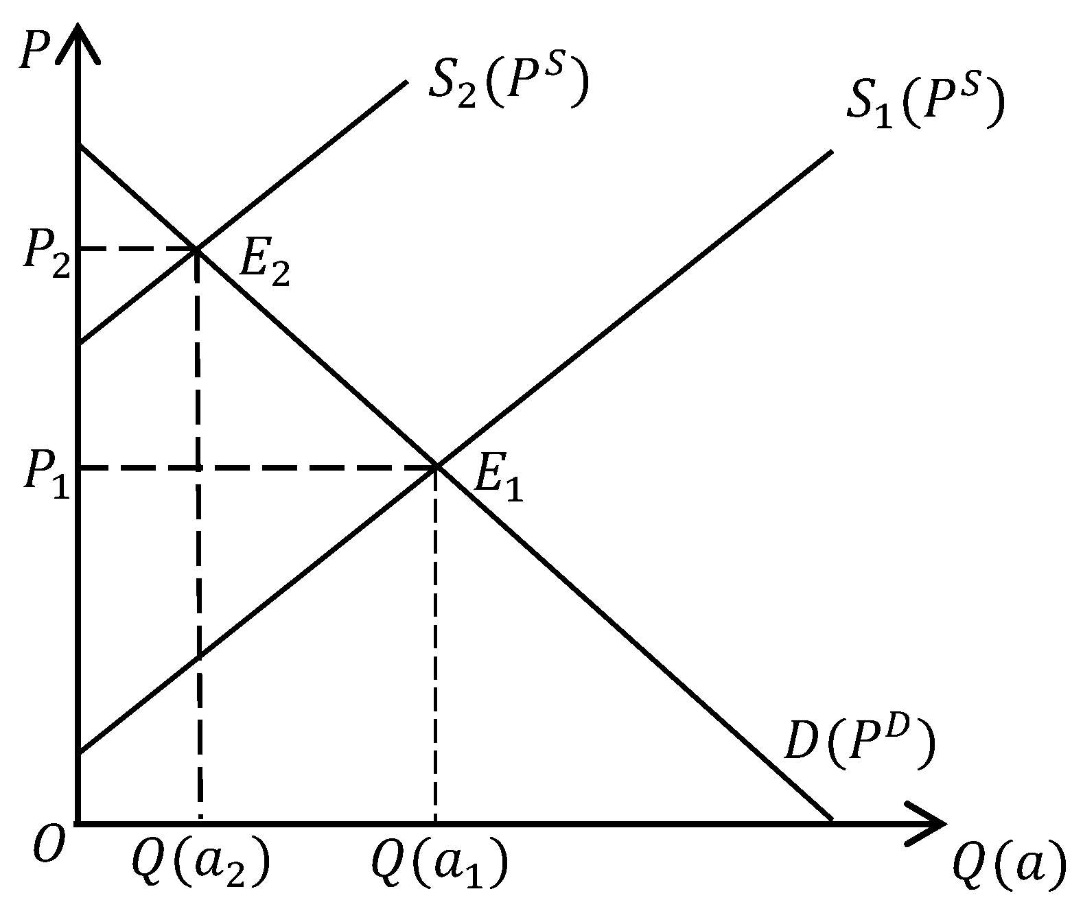
Appendix B
Figure A1 describes the shift in supply curves and market equilibrium of agricultural products.
and
denote the prices and quantities of agricultural products.
and
denote the demand curve and supply curve of agricultural products, respectively.
and
are the market equilibrium points when the supply curve moves to
and
. The triangular areas formed by the supply curve, the demand curve and the vertical axis are the total economic surplus, the areas above the equilibrium price are consumer surplus and below the equilibrium price are producer surplus.
Figure A1.
Shift in supply curves and market equilibrium.
Figure A1.
Shift in supply curves and market equilibrium.
Appendix C
Referring to Yi et al. (2018) [
19], we introduced the structure of CASM in detail. The agricultural production possibilities for crop and livestock production, are denoted as
; subscript
represent China’s trading partner countries, subscript
and
represent subregions in China;
represents inputs used for commodity production and
nutrients derived from farm family consumption of farm produced products. The regional economic optimization model for China’s agricultural sector is defined as follows (The full model is written using GAMS.) and the definitions of parameters and variables are listed in
Table A6 and
Table A7.
Table A6.
Definitions of Parameters.
Table A6.
Definitions of Parameters.
| Parameters | Definitions |
|---|
| Yield of production activity in region in period |
| Unit cost of storage by farmers for commodity in region |
| Unit cost of storage for commodity in market |
| Unit cost of transportation for commodity |
| Subsidy for commodity in region |
| Endowed amount of input in region , such as land, family, and labor |
| Amount of family labor supply in region |
| Amount of labor from region that can be supplied to labor market |
| Minimum requirement of nutrient in region arising from on-farm consumption for human beings and livestock in a period |
| Content of nutrient in commodity |
Table A7.
Definitions of Variables.
Table A7.
Definitions of Variables.
| Variables | Definitions |
|---|
| Annual country-wide, total, non-farm, domestic demand for commodity that is bought from market |
| Amount of commodity that is used at the farm level from the farmers’ own production being either consumed by the farm family or farm livestock in region in period |
| Share of non-farm consumption for commodity that occurs in period |
| Amount of commodity exported annually |
| Amount of commodity exported in period |
| Amount of commodity imported annually |
| Amount of commodity imported in period t |
| Amount of commodity stored by farmers in region in period t |
| Amount of commodity stored in market in period |
| Amount of commodity moved out from region to region in period t |
| Inverse non-farm demand function for commodity |
| Inverse supply function for purchased factor |
| Inverse supply function for imports of commodity |
| Inverse demand function for exports of commodity |
| Amount of hired labor supplied in region |
| Inverse supply function for hired labor in region |
| Quantity of purchased factor |
| The level of production activity in region , such as planted area of a crop or number of heads of a type of livestock |
| Amount of input used for the production of commodity in region |
| Amount of labor used to produce one unit of production item in region |
| Amount of labor migrating out from region to other regions |
| Amount of labor migrating into region from other regions |
The model maximizes consumers’ and producers’ surplus in Equation (A1) subject to market supply-demand balances, resource, and family nutritional constraints. Equation (A2) presents the aggregate demand-and-supply balance for China’s domestic agricultural commodity market by period. The equation shows that the demand fora specific commodity includes domestic consumption, commodities transported out to regional markets, exports, and storage into the next period. Supply comes from commodities transported in from production regions, imports, and storage from the last period. Demand is less than or equal to the total supply. As agricultural production and consumption occur over time, the market-clearing conditions are represented for each month. To simplify the model, the monthly share of non-farm consumption is set as 1/12 the annual estimate. Equation (A3) shows the regional demand-and-supply balance by period. The demand includes farmers’ self-consumption, the amount of a commodity transported from each region to other regions, and storage into the next period. Local supply is from production, commodities transported in from other regions to this region , and storage from the last period. Equation (A4) is a resource-endowment constraint for each sub-region, restricting the use of land and family labor in agricultural production to be less than or equal to the total available land and family labor endowment, respectively. On rice production, a regional land suitable for maximum paddy land available is added to restrain rice to only flat lands with water access. Inequality (A5) states that the total amount of labor used in agricultural production should be less than or equal to the aggregate amount available from the two sources of labor, namely, family labor and hired labor from the market. This inequality is a market-clearing condition that is similar to Constraint (A2) but only for labor. Inequality (A6) requires that regional labor hired be no more than local labor market supply. Constraint (A7) captures the nutrition requirements for the family and livestock on a regional, monthly, and nutrient basis. For farm families, we assume that 60% of calories and protein comes from on-farm grain consumption. In the average Chinese diet, about 65% of the calories come from rice. For crops fed to livestock, multi-commodity diet alternatives are entered for each different animal types, and the model chooses the optimum. Generally, maize and soybeans are the most important feeds for livestock. Equations (A8) and (A9) require the aggregates of monthly imports and exports to be equal to the annual values of trade.
Appendix D
Table A8.
Calibration between observed and model-generated production and price.
Table A8.
Calibration between observed and model-generated production and price.
| Commodities | Production Level in Terms of Planted Area (1000 ha)/Livestock Numbers (1000 Head) | Price (CNY/kg) |
|---|
| Observed | Model | % Deviation | Observed | Model | % Deviation |
|---|
| Rice | 28,845.9 | 29,677.9 | 2.9 | 2.0 | 2.1 | 4.5 |
| Wheat | 26,869.8 | 28,198.5 | 4.9 | 1.6 | 1.7 | 4.9 |
| Maize | 41,248.5 | 42,816.3 | 3.8 | 1.6 | 1.7 | 3.7 |
| Soybean | 6218.0 | 6305.2 | 1.4 | 3.5 | 3.5 | 1.6 |
| Peanut | 4619.6 | 4563.3 | −1.2 | 6.0 | 6.0 | −0.7 |
| Rapeseed | 7633.4 | 7455.3 | −2.3 | 3.5 | 3.5 | −0.7 |
| Cotton | 4100.7 | 4114.8 | 0.3 | 10.6 | 10.6 | 0.6 |
| Tobacco | 1463.2 | 1504.9 | 2.9 | 15.3 | 16.0 | 4.0 |
| Sugarcane | 1756.5 | 1756.7 | 0.0 | 0.4 | 0.4 | 0.0 |
| Sugar beet | 117.1 | 117.0 | −0.1 | 0.4 | 0.4 | −0.2 |
| Potato | 9401.7 | 9538.6 | 1.5 | 0.9 | 0.9 | 1.7 |
| Fiber crops | 83.0 | 82.2 | −0.9 | 6.8 | 7.0 | 2.4 |
| Other grain crops | 3025.2 | 3150.1 | 4.1 | 5.8 | 6.0 | 5.0 |
| Vegetable and cucurbits | 21,842.5 | 21,848.1 | 0.0 | 1.4 | 1.4 | 0.1 |
| Other beans | 1391.2 | 1357.8 | −2.4 | 3.2 | 3.2 | −0.6 |
| Other oil crops | 1556.6 | 1554.1 | −0.2 | 6.0 | 6.0 | 0.0 |
| Hen | 16,556.1 | 16,538.5 | −0.1 | 5.8 | 5.9 | 0.7 |
| Broiler | 120,770.5 | 118,624.1 | −1.8 | 12.7 | 12.7 | 0.6 |
| Cattle | 47,609.0 | 47,536.5 | −0.2 | 48.2 | 48.3 | 0.2 |
| Cow | 6587.3 | 6590.5 | 0.0 | 2.7 | 2.7 | 0.4 |
| Hog | 697,896.0 | 698,863.5 | 0.1 | 16.0 | 16.1 | 0.4 |
| Sheep | 270,998.0 | 270,008.5 | −0.4 | 52.1 | 52.2 | 0.3 |
Appendix E
In the absence of an ENSO forecast, the crop production under each realized ENSO phase can be obtained from the remaining planting acreage and average yields for each realized ENSO phase. The long-term expected crop production can be obtained based on the production under each realized ENSO phase by averaging over
. When the ENSO forecast is provided, we acquire crop production under each realized ENSO phase for the given predicted ENSO phase according to the planting acreages for each predicted ENSO phase and average yields for each realized ENSO phase. The long-term expected crop production for the scenario with ENSO forecast is derived by averaging over
and
. The framework is similar to the calculation of expected economic surplus in
Section 3, and the formulas are listed as follows:
where
is the expected crop production without ENSO forecast and
is the expected crop production in the presence of ENSO forecast.
denotes the average yield for each realized ENSO phase estimated in
Section 2 inprefecture-level city
c. Let
be the remaining planting acreage without ENSO forecast inprefecture-level city c and
is the planting acreage for each predicted ENSO phase in prefecture-level city
c. The national crop production is calculated by summing that of the 365 prefecture-level cities.
References
- Guo, J. Advances in impacts of climate change on agricultural production in China. J. Appl. Meteorol. Clim. 2015, 26, 1–11. (In Chinese) [Google Scholar]
- Tack, J.B.; Ubilava, D. Climate and agricultural risk: Measuring the effect of ENSO on US crop insurance. Agric. Econ. 2015, 46, 245–257. [Google Scholar] [CrossRef]
- Tack, J.B.; Ubilava, D. The effect of El Niño Southern Oscillation on US corn production and downside risk. Clim. Chang. 2013, 121, 689–700. [Google Scholar] [CrossRef]
- Ubilava, D.; Barnett, B.J.; Coble, K.H.; Harri, A. The SURE program and its interaction with other federal farm programs. J. Agric. Resour. Econ. 2011, 36, 630–648. [Google Scholar]
- Solow, A.R.; Adams, R.M.; Bryant, K.J.; Legler, D.M.; O’Brien, J.J.; McCarl, B.A.; Nayda, W.; Weiher, R. The Value of Improved ENSO Prediction to U.S. Agriculture. Clim. Chang. 1998, 39, 47–60. [Google Scholar] [CrossRef]
- Adams, R.M.; Houston, L.; McCarl, B.A.; Tiscareño, M.L.; Matus, J.G.; Weiher, R.F. The benefits to Mexican agriculture of an El Niño-Southern Oscillation (ENSO) early warning system. Agric. For. Meteorol. 2003, 115, 183–194. [Google Scholar] [CrossRef]
- Just, R.E.; Weninger, Q. Are crop yields normally distributed? Am. J. Agric. Econ. 1999, 81, 287–304. [Google Scholar] [CrossRef]
- Chen, S.-L.; Miranda, M.J. Modeling Multivariate Crop Yield Densities with Frequent Extreme Events. In Proceedings of the American Agricultural Economics Association Annual Meeting, Denver, CO, USA, 1–4 August 2004. [Google Scholar]
- Goodwin, B.K.; Mahul, O. Risk Modeling Concepts Relating to the Design and Rating of Agricultural Insurance Contracts; World Bank Policy Research Working Paper No. 3392; The World Bank: Washington, DC, USA, September 2004. [Google Scholar]
- Harri, A.; Goodwin, B.J. Relaxing heteroscedasticity assumptions in area-yield crop insurance rating. Am. J. Agric. Econ. 2011, 93, 703–713. [Google Scholar] [CrossRef]
- Zhang, Y. A density-ratio model of crop yield distributions. Am. J. Agric. Econ. 2017, 99, 1327–1343. [Google Scholar] [CrossRef]
- Goodwin, B.K.; Ker, A.P. Nonparametric estimation of crop yield distributions: Implications for rating group-risk crop insurance contracts. Am. J. Agric. Econ. 1998, 80, 16. [Google Scholar] [CrossRef]
- Nelson, C.H.; Preckel, P.V. The conditional Beta distribution as a stochastic production function. Am. J. Agric. Econ. 1989, 71, 370–378. [Google Scholar] [CrossRef]
- Gallagher, P.U.S. soybean yields: Estimation and forecasting with nonsymmetric disturbances. Am. J. Agric. Econ. 1987, 69, 8. [Google Scholar] [CrossRef]
- Nadolnyak, D.; Vedenov, D.; Novak, J. Information value of climate-based yield forecasts in selecting optimal crop insurance coverage. Am. J. Agric. Econ. 2008, 90, 1248–1255. [Google Scholar] [CrossRef]
- Kite-Powell, H.L.; Solow, A.R. A Bayesian approach to estimating benefits of improved forecasts. Meteoro. Appl. 1994, 1, 351–354. [Google Scholar] [CrossRef]
- Samuelson, P.A. Spatial price equilibrium and linear programming. Am. Econ. Rev. 1952, 42, 283–303. [Google Scholar]
- McCarl, B.A.; Spreen, T.H. Price endogenous mathematical programming as a tool for sector analysis. Am. J. Agric. Econ. 1980, 62, 87–102. [Google Scholar] [CrossRef]
- Yi, F.; McCarl, B.A. Increasing the effectiveness of the Chinese grain subsidy: A quantitative analysis. China Agric. Econ. Rev. 2018, 10, 538–557. [Google Scholar] [CrossRef]
- Yi, F.; McCarl, B.A.; Zhou, X.; Jiang, F. Damages of surface ozone: Evidence from agricultural sector in China. Environ. Res. Lett. 2018, 13, 034019. [Google Scholar] [CrossRef]
- Adams, R.M.; Hamilton, S.A.; McCarl, B.A. The benefits of pollution control: The case of ozone and US Agriculture. Am. J. Agric. Econ. 1986, 68, 886–893. [Google Scholar] [CrossRef]
- Howitt, R.E. Positive mathematical programming. Am. J. Agric. Econ. 1995, 77, 329–342. [Google Scholar] [CrossRef]
- Chen, B. The Study on Chinese Grain Security Cost and it’s Structure Optimization. Ph.D. Thesis, Huazhong Agricultural University, Wuhan, China, 2007. (In Chinese). [Google Scholar]
- Feng, J.; Zhang, T. Labor supply elasticity of migrant workers. J. Quant. Tech. Econ. 2012, 10, 69–82. (In Chinese) [Google Scholar]
- Zhang, Z. A solution to improve the profits of agricultural sector. Sci. Technol. Rev. 2004, 22, 49–51. (In Chinese) [Google Scholar]
- Barrett, C.B. The value of imperfect ENSO forecast information: Discussion. Am. J. Agric. Econ. 1998, 80, 1109–1112. [Google Scholar] [CrossRef]
- Lau, K.M.; Yang, S. The Asian monsoon and predictability of the tropical ocean–atmosphere system. Q. J. Roy. Meteor. Soc. 1996, 122, 945–957. [Google Scholar]
- Kirtman, B.; Shukla, J.; Balmaseda, M.; Graham, N.; Penland, C.; Xue, Y.; Zebiak, S. Current Status of ENSO Forecast Skill: A Report to the CLIVAR Working Group on Seasonal to Interannual Prediction; WCRP Informal Report No 23/01, ICPO Publication Ser. 56; International CLIVAR Project Office: Southampton, UK, 2001. [Google Scholar]
- McPhaden, M.J. Tropical Pacific Ocean heat content variations and ENSO persistence barriers. Geophys. Res. Lett. 2003, 30. [Google Scholar] [CrossRef] [Green Version]
- Duan, W.; Wei, C. The ‘spring predictability barrier’for ENSO predictions and its possible mechanism: Results from a fully coupled model. Int. J. Climatol. 2013, 33, 1280–1292. [Google Scholar] [CrossRef]
- Shuai, J.; Zhang, Z.; Sun, D.-Z.; Tao, F.; Shi, P. ENSO, climate variability and crop yields in China. Cli. Res. 2013, 58, 133–148. [Google Scholar] [CrossRef]
- Zhang, T.; Zhu, J.; Yang, X.; Zhang, X. Correlation changes between rice yields in North and Northwest China and ENSO from 1960 to 2004. Agric. For. Meteorol. 2008, 148, 1021–1033. [Google Scholar] [CrossRef]
- Zheng, D.; Yang, X. Advances on effect of ENSO on agro-meteorological disasters and crop yields of the world and China. Meteorol. Environ. Sci. 2014, 37, 90–101. (In Chinese) [Google Scholar]
- Iizumi, T.; Luo, J.-J.; Challinor, A.J.; Sakurai, G.; Yokozawa, M.; Sakuma, H.; Brown, M.E.; Yamagata, T. Impacts of El Niño Southern Oscillation on the global yields of major crops. Nat. Commun. 2014, 5, 1–7. [Google Scholar] [CrossRef]
- Liu, Y.; Yang, X.; Wang, E.; Xue, C. Climate and crop yields impacted by ENSO episodes on the North China Plain: 1956–2006. Reg. Environ. Chang. 2014, 14, 49–59. [Google Scholar] [CrossRef]
- Chi-Chung Chen, B.A.M. The value of ENSO information to agriculture: Consideration of event strength and trade. J. Agric. Resour. Econ. 2000, 25, 368–385. [Google Scholar]
© 2019 by the authors. Licensee MDPI, Basel, Switzerland. This article is an open access article distributed under the terms and conditions of the Creative Commons Attribution (CC BY) license (http://creativecommons.org/licenses/by/4.0/).


