Abstract
The paper presents the results of the effects of control drainage (CD) on the groundwater table and subsurface outflow in Central Poland. The hydrologic model DRAINMOD was used to simulate soil water balance with drain spacing of 7 and 14 m, different initial groundwater Table 40, 60 and 80 cm b.s.l., and dates at the beginning of control drainage of 1 March, 15 March, 1 April, and 15 April. The CD restricts flow at the drain outlet to maintain a water table during the growing season. Simulations were made for the periods from March to September for the years 2014, 2017, and 2018, which were average, wet, and dry, respectively. The simulations showed a significant influence of the initial groundwater tables and date blocking the outflow from the drainage network on the obtained results. In the conditions of central Poland, the use of CD is rational only when it is started between 1 and 15 March. In this case, the groundwater table can be increased from 10 to 33 cm (7 m spacing) and from 10 to 41 cm (14 m spacing) in relation to the conventional system (free drainage—FD). In the case of blocking the outflow on 1 March, the reduction is about 80% on average in the period from March to September. With a delay in blocking the outflow, the impact of CDs decreases and ranges from 8% to 50%. Studies have shown that the proper use of the drainage network infrastructure complies with the idea of sustainable development, as it allows efficient water management, by reduction of the outflow and, thus, nitrates from agricultural areas. Furthermore, CD solutions can contribute to mitigating the effects of climate change on agriculture by reducing drought and flood risk.
1. Introduction
Climate change is being observed all over the world. On the scale of individual continents, its direction and extent vary. Countries located in central Europe, including Poland, will be exposed to extreme temperatures and reduced precipitation in the summer [1]. The temperature increase and changes in rainfall temporal distribution lead to increased risk of floods, droughts, and heat waves [2,3]. The consequence will be that dry regions are becoming even drier, and drought hazards are increasing [4]. A significant reduction in surface water and groundwater resources will cause all water users to be affected by the consequences of climate change in different way [5]. Consequently, this will lead to exacerbated competition among water users and sectors [6].
One of the main challenges for sustainable development is the adaptation of national economies to climate change. Most often, climate change adaptation projects in Poland are carried out in cities and areas subject to urban sprawl [7,8,9]. Agriculture is a key sector for food supply, and its functioning depends largely on access to water. It is, therefore, necessary to take various actions to protect this sector of national economies against climate change. The most frequently asked question is whether and to what extent it is possible to take action in the adaptation of agriculture to climate change while maintaining high environmental standards and accounting for the acceptance of society and economic balance.
The greatest scope for the mitigation of the effects of climate change is in improving adaptive capacity and responding to changes in water demands [10]. Agricultural subsurface drainage, popularly known as tile drainage, is an essential water management practice in agricultural regions with seasonal high groundwater tables [11]. Around 193.9 × 10⁶ ha of arable land, and permanent crops have been drained around the world. In 30 countries, the total drained area is more than 1.0 ·106 ha [12]. In Poland, subsurface drainage systems were developed in the period from 1950 to 1990 for a total of 4.2 × 10⁶ ha drained, which accounts for about 30% of arable land. Heavy soils were mainly drained, on which there was periodical excess of water after spring snowmelt and after intensive precipitation in summer. In Poland, the drainage system removes excess water and does not allow blockage of the outflow. Drought mitigation plans developed in Poland emphasize the potential of drainage systems. Attention is paid to the possibility of adapting the existing infrastructure to perform new functions that were not previously taken into account at the design stage. Thus, there is an urgent need to change from free drainage (FD) to control drainage (CD) systems by equipping them with facilities for blocking water in a tile drain. This will allow water to be stored efficiently where it is needed most. In some countries, control drained solutions are used as the best management practice for good agriculture. For this purpose, the drainage network has been supplemented with a simple water level control structure. This makes it possible to control the outlet elevation at different times during the year according to crop stage and water needs [13]. Drainage water management (DWM), controlled tile drainage (CTD), and controlled drainage (CD) are promoted as agricultural best management practices that reduce subsurface outflow and export nutrients [14,15,16,17,18,19,20].
Field studies are being carried out to assess the impact of the CD solution. The results of these studies are usually of a local character. Therefore, they are used to identify the parameters of models, their calibration, and their verification. The models developed in this way allow for the assessment of various scenarios of water management in a drainage network under current and future climatic conditions. Over the years, in the world, several process-based models have been developed to simulate the soil–water–plant relationship. Examples of these models include DRAINMOD [21] and its subsequent updates, DRAINMOD-N [22], DRAINMOD-NII [23], and DRAINMOD-DSSAT [24]. The DRAINMOD model is commonly used worldwide, to simulate the soil water balance and predict subsurface drainage, surface runoff, infiltration, deep seepage, water table depth, and evapotranspiration, as affected by changes in weather conditions, crop cover, soil type, and drainage system design [24,25,26,27,28,29,30]. DRAINMOD-NII is a companion model to DRAINMOD [23]. DRAINMOD-NII is a process-based model that simulates the carbon (C) and nitrogen (N) dynamics of drained cropland. Negm et al. [24] stated that the integrated agricultural system model DRAINMOD-DSSAT is an effective research tool to show drained fields’ response to varying climatic conditions in the context of agricultural production and environmental quality. DRAINMOD-DSSAT was developed to simulate hydrology, soil carbon and nitrogen dynamics, and crop growth. The impact of CD on outflow reduction was well predicted by the model [19]. Skaggs et al. [31,32] demonstrated that the effectiveness of the DWM practice depends on soils, climatic conditions, and drainage system design and management. Moreover, it is important to identify the parameters of the model, especially in respect to soil properties [33].
The implementation of CD solutions to agricultural practice in Poland, but also in other countries, considering climate and soil conditions, requires both field experiments and model studies. To determine the effects of these CD solutions, field studies and computer simulations should be carried out. This will help to answer the question of how much these solutions may increase the groundwater table and reduce subsurface outflow and, consequently, mitigate the effects of climate change on the agricultural sector. The aim of the study was to evaluate various scenarios of CD in groundwater table dynamics and subsurface outflow on the field scale. Simulations were performed with the assumption of different weather conditions (dry, normal and wet period), initial groundwater table conditions (initial water table depth), drainage network parameters (drainage spacing), and CD practices (dates of the beginning of blocking the outflows). The main aim of the study was to determine the possibility of using CDs in Polish conditions, where such research had not been conducted before. The research presented in the paper is a preliminary part of a project financed by the National Centre for Research and Development in Poland, entitled “Technological innovations and system of monitoring, forecasting and planning of irrigation and drainage for precise water management on the scale of drainage/irrigation system (Acronym—INOMEL)”. The aim of the project is to develop operational CD management plans adjusted to the water needs of plants and the dates of field work based on hydrological and meteorological monitoring and hydrometeorological forecasts. Moreover, this research will answer the question of whether and to what extent it is possible to use CDs in the aspect of agricultural mitigation for climate change. This research is also important in the context of the implementation of the Water Framework Directive and the Nitrates Directive. The Directives oblige EU Member States to achieve good water status by limiting nitrogen outflow from agricultural areas.
2. Materials and Methods
2.1. Study Site Description
Field studies were carried out on arable land located in the central part of Poland (52°21′38.5′′ N, 17°36′34.2′′ E) (Figure 1). The research area is one of the most water deficient areas in Poland [34]. The average annual rainfall from 1981–2018 was 542 mm, and the average annual air temperature was 9.1 °C. The research was carried out in a tile drainage system with an area of approximately 107 ha, which was built in the 1980s. The drainage network was made of PVC pipes. There are 22 drainage sections with an area of 2.53 ha (drainage section no. 34) to 12.54 ha (drainage section no. 38). The drainage network is located at a depth of 0.9 to 1.0 m. b.s.l., and the spacing between the drains is usually 14 m. The drainage spacing is 7 m only on sub-sections 42_2 and 42_3. Water from the drainage section is directed to the ditches by means of drainage outlets (17 outlets in the whole system—green circle) or to drainage wells (10 outlets in the whole system—blue circle), which are connected by a pipeline to the ditches. Both in wells and drainage outlets there is a possibility of using DWM solutions. The survey area is characterized by low relief diversity, slopes do not exceed 5‰, and the difference between the highest and the lowest point is 6.44 m. In this study, the results of studies carried out in drainage section no. 42 was used. This section was divided into four parts. In parts 42_1 and 42_4, the drainage spacing is 14 m, and in parts 42_2 and 42_3, the spacing is 7 m. The devices for control drainage in the wells located in sections 42_1 and 42_2 were installed. The sections 42_3 and 42_4, on the other hand, are an FD network—without to possibility to block the outflows (free drainage). Since February 2019, these wells have been used for water table and flow rate measurements with a frequency of 10 min. The soils occurring within the analyzed drainage sections were classified as Gleyic Luvisols [35], which were developed from glacial till. Both the surface and subsurface horizons have a sandy loam texture, but the argic horizon has distinctly higher clay content than the overlying horizons.
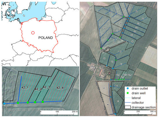
Figure 1.
Study site location.
2.2. Model Description
DRAINMOD is a hydrologic model used to simulate a soil-water balance on tile drained fields [21]. The water balance is calculated to unit surface area which is a vertical soil column. The column extends from the soil surface down to the impermeable layer and is located midway between two adjacent drains. The water balance of the soil column can be written as
where ∆Va is the change in the water-free pore space or air volume (mm), I is the infiltration (mm), ET is the evapotranspiration (mm), LD the lateral drainage (the negative sign—outflow for subsurface drainage, and the positive sign—inflow for subirrigation) (mm), and DS is the deep seepage (the negative sign for downward movement—the outflow to lower layers; and the positive sign for upward movement—inflow from lower layers) (in mm).
ΔVa = I − ET ± LD ± DS,
A water balance is also computed at the soil surface and can be written as:
where P is the precipitation (mm), SR the surface runoff (mm), and ∆S is the surface water storage change (mm). The calculations are performed for a time increment Δt. The rates of I, ET, LD, and DS are computed by commonly used methods that have been used for a range of soil and boundary conditions. The infiltration is calculated by the Green–Ampt equation. The daily potential evapotranspiration (PET) is calculated by the Thornthwaite [36] method. Next, the PET is reduced to actual evapotranspiration (ET), depending on the weather and soil water conditions. The LD is calculated with Hooghoudt’s steady state equation, with a correction for convergence near the drains [37]. The LD from a ponded surface is calculated using the equation derived by Kirkham [38]. The DS rates are calculated with a straightforward application of Darcy’s law. The detailed description of soil water distribution processes in DRAINMOD (which assumes two zones, a wet zone and a dry zone) is given by Skaggs [39].
P = I + SR + ΔS
2.3. Methods
In order to assess the impact of DWM on groundwater tables and subsurface outflow from the tile drainage, the research was divided into three stages. In the first stage, data were collected and arranged into a homogeneous geodatabase in accordance with the requirements of the DRAINMOD model. In the second stage, the model parameters were identified, and then the model was calibrated and validated. The model prepared in this way was used to simulate various scenarios of the network operation. In the third stage, the results were statistically analysed. The research procedure is presented in Figure 2.
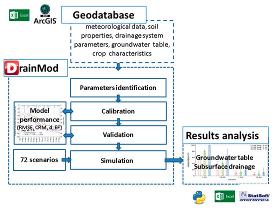
Figure 2.
Research procedure.
2.4. Data Collection and Geodatabase Creation
Initially, maps of the presented drainage system were obtained. The maps were made at a scale of 1:2000, at which the drainage network was shown. The maps were scanned and then vectorised in the ArcGIS software. Additionally, soil maps at a scale of 1:5000 were obtained, and a digital elevation model (DEM) with a resolution of 1 m was developed on the basis of data from airborne laser scanning. Soil maps and DEM were obtained from the Central Office of Geodesy and Cartography in Poland. Moreover, the archives of the Institute of Land Improvement, Environmental Development and Geodesy, Poznań Life Sciences University obtained data from field measurements carried out during the 1988–2003 period. These archives included physical soil and water properties in drainage section no. 42, periodical measurements of groundwater tables and the subsurface outflow from the drainage network in sections 42_1 to 42_4, daily measurements of air temperature and precipitation, as well as information on the crop structure in section 42.
2.5. Drainage Water Management Simulation
The model parameters were identified on the basis of data collected at the first stage of study. The main input parameters describing the drainage system used for DRAINMOD simulations are presented in Table 1. The crop parameters were determined on the basis of data provided by Feddes et al. [40] and Van Dam et al. [41].

Table 1.
Input parameters specified for DRAINMOD simulations.
Soil water retention curves of the undisturbed core soil samples up to 100 kPa were made using the Richards chambers, whereas lower values of the pressure head were performed using the method of water vapour pressure over a solution of sulphuric acid [42,43]. Following this, the RETC program [44] was used to present the soil water retention curve in the form of the parameters of the Van Genuchten [44] equation with the Mualem [45] assumption (m = 1 − 1/n, where m and n are parameters of Van Genuchten equations). The filtration coefficient was determined using the method of a constant hydraulic water gradient [46]. The soil utility package included in DRAINMOD was used to estimate the Green–Ampt infiltration model parameters, the drainage volume–water table depth, and the water upflux–water table depth relationships. Basic soil properties and hydraulic parameters are presented in Table 2.
Table 2.
Soil properties and hydraulic parameters.
2.6. Model Calibration and Validation
Calibration and verification of the model was performed according to the procedure described by Skaggs et al. [47]. At this stage, measurement data from the growing season of 2000 were used. Then, the model was validated on the basis of measurement data from 1994. Calibration and validation of the model are key procedures in reducing prediction uncertainty. During the calibration process, the model’s input parameters were changed to obtain the optimum agreement between the predicted and observed variables [48,49]. Three parameters—hydraulic conductivity by layer Ksat (cm.day−1), the thickness of the restrictive layer, and the hydraulic head at the bottom of the restrictive layer—were adjusted to minimize the difference between the observed and predicted water tables. The quality of the DRAINMOD simulation model to determine the groundwater table dynamics in drained soils was analysed using commonly used statistical measures, such as the root mean square error (RMSE), coefficient of mass residual (CRM), index of agreement, (d) and model efficiency index (EF) [48,49]. These parameters are defined as
where n is the total number of the observations, Oi is the observed value of the ith observation, Pi the predicted value of the ith observation, and O the mean of the observed values (i = 1 to n). The RMSE and CRM have smaller values when the values predicting the ith obtained measurements are more consistent. The EF and d value for the optimal adjustment of the predicted and observed values were close to 1 [47,49]. The threshold values for acceptable, good, and excellent agreement for water table depth were established on the basis of Skaggs et al. [47].
2.7. Drainage Water Management Simulations
Simulations were performed with the assumption of different meteorological conditions (dry, normal, and wet periods), initial groundwater table conditions (on 1 March—the start of the simulation), drainage network parameters (drainage spacing 7 and 14 m), and the dates of the beginning of CD practice (1 and 15 March and 1 and 14 April) (Table 3). Damming height is the outlet height of the water level control structure below the surface level. A total of 72 simulations were carried out.
Table 3.
Simulation scenarios.
Simulations were performed for the periods from 1 March to 30 September. Three years, 2014, 2017, and 2018, were chosen for the simulation. These dates were characterized by different thermal and precipitation conditions. The general characteristics of the meteorological conditions in the selected years are presented in Table 4.
Table 4.
Yearly total and simulating period (March 1 to September 30) precipitation and average temperature.
Three different initial conditions were established. The simulation was performed for dry, normal, and wet years. The initial groundwater table in 1 March at 0.80 m b.s.l. means that the year preceding the simulation was dry, whereas, in the case of the initial state of 0.40 m b.s.l., the year preceding the simulation was wet. This allows the whole spectrum of possible situations to be taken into account.
2.8. Statistical Analysis
In order to compare the results of the 72 simulations, a script in the Python 3.7.3 language was developed. This script allowed for the automatic recording of the depth of groundwater and subsurface outflows from the tile drainage in an Excel spreadsheet. The aim of the statistical analysis was to compare the depth of the groundwater in the case of conventional solutions and controlled drainage. Groundwater analysis was performed for the whole simulation period (March to September) and for individual months. For each variant, groundwater table duration curves were developed, from which the time of the groundwater above the drainage network was determined. The number of days with subsurface outflow and the effect of different variants of controlled drainage were also determined and compared. In order to assess the statistical differences in the groundwater table in different variants of controlled drainage, a non-parametric analysis of the variance was performed using the STATISTICA 13.1 PL statistical software, with Kruskal–Wallis (K–W) and Dunn’s tests as post hoc procedures (p ≤ 0.05).
3. Results
The parameters of the model were identified, and then the model was calibrated and validated before starting the simulation. The DRAINMOD model was calibrated and validated using groundwater table data for the years 1994 and 2000. The results of the groundwater table depth in the year 2000 were used to calibrate the model. Data from 1994 were used to validate the model. Calibration and validation of the model was carried out for a drainage system working in a conventional way (free drainage—FD), without CD solutions. The model was calibrated with the trial and error method by adjusting the hydraulic conductivity by layer, the thickness of the restrictive layer, and the hydraulic head at the bottom of the restrictive layer, one after the other, within reasonable ranges. This allowed for good agreement between the results of the simulation from the DRAINMOD model and the results of groundwater measurements from 2000. In the next stage, the model was validated based on the data of the groundwater table from 1994. The results of the calibration and validation procedure are presented in Table 5. The RMSE, CRM, d, and EF values show excellent agreement between the measured and predicted groundwater tables. This result proves that a model set up in this way can be used to simulate the impact of various CD scenarios on groundwater table dynamics and the subsurface outflow of drained soils.
Table 5.
Statistical performance of the DRAINMOD model to predict the groundwater table in the years 1994 and 2000.
In the next stage, in order to assess the impact of CDs on groundwater tables and subsurface outflow from the drainage network, a series of simulations was carried out according to the previously established scheme. The precipitation from March to September varied from 252 mm in 2018 to 523 mm in 2017 (Table 4). In 2018, the highest temperature (15.0 °C) was recorded with the lowest total precipitation. Also in the years 2014 and 2017 the temperatures were higher than the average value for the years 1981–2018.
During the simulation procedure, the measured daily precipitation was uniformly distributed over 6 h (from 15 to 21 h) to obtain the hourly precipitation required in DRAINMOD. This procedure is described by Skaggs et al. [47] and Ale et al. [11]. The ET value calculated by the Thornthwaite method was corrected using the monthly ET factors. The following monthly ET factors for the growing season were used during the simulation (March 1 to September 30): 0.6 (March) 0.7 (April) 0.9 (May), 1.0 (June–July), 0.9 (August), 0.8 (September).
The results of the simulations produced daily groundwater tables and subsurface outflows from the tile drainage for the period from March to September (Figure 3). A total of 72 simulations were performed, of which 18 were the reference level, because they assumed that the drainage network functions in a conventional way without the possibility of blocking the outflow (free drainage—FD).
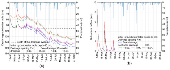
Figure 3.
Impact of CD on (a) depth of the groundwater table and (b) the subsurface drainage rate in 2014, assuming an initial groundwater table depth on 1 March 40 cm b.s.l. and drain spacing of 7 m.
Taking into account the different conditions of the groundwater table at the beginning of the simulation period (1 March), and the precipitation and air temperature conditions in 2014, 2017, and 2018, the FD system allows for the unproductive removal of water. Groundwater was located above the level of the drainage network for 27 to 51 days in the case of the 7 m drain spacing and for 40 to 66 days in the case of the 14 m drain spacing. The use of CD solutions allows one to extend the period in which the groundwater table is located above the drainage network. The most effective method is to start stopping the outflow on 1 March. In this way, it is possible to extend the period of the groundwater above the level of the drainage network. When a CD solution was used in a drainage network with a spacing of 7 m, the time that the groundwater was above the drainage network ranged from 74 to 113 days (average 94 days), and in a network with a spacing of 14 m, it ranged from 74 to 115 days (average 100 days). Slightly worse results were obtained for the scenarios in which the CD solution started on 15 March. Even less important are the CD procedures, which further delayed the start of blocking the outflow from the drainage network. Starting to block out the outflow from the drainage network with a spacing of 7 m on 1 April or 15 April means that the time of groundwater location above the drainage can be extended by 13 and 7 days, respectively. A slightly better result can be achieved with 14 m network spacing. Starting to block the outflow on 1 or 15 April will increase the time of groundwater accumulation above the drains by 17 and 7 days, respectively (Figure 4).
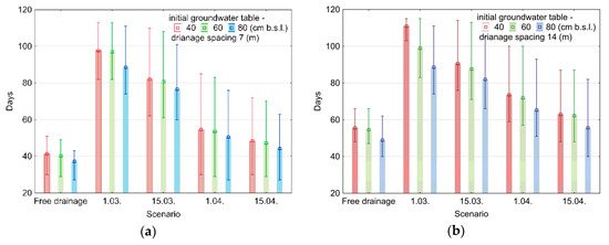
Figure 4.
Impact of different variants of controlled drainage on the time the groundwater table is above the level of the drainage network with a spacing of 7 m (a) and 14 m (b) (bar charts show the average values, as well as the minimum and maximum values for the years 2014, 2017, and 2018).
The impact of CD solutions on groundwater is illustrated well by the curves of the groundwater table duration. The most effective CD solutions are effective when starting to block the outflow on 1 March (red line) with a high initial groundwater table of 40 and 60 cm b.s.l. (Figure 5a,b and Figure 6a,b). The figures show that the groundwater tables in the case of the conventional network (free drainage (FD), dark blue line) are at the same level as if the blocking of the outflow had started on 1 or 15 April (purple and black lines). The 7 m spacing of the drainage system allows faster drainage and, in this case, delayed blocking of the outflow means that all the water from the field is drained in March. In the case of a drainage network with a spacing of 14 m, the differences between the groundwater table when blocking the outflow on 1 or 15 March are at a lower level than those for a network with a spacing of 7 m.
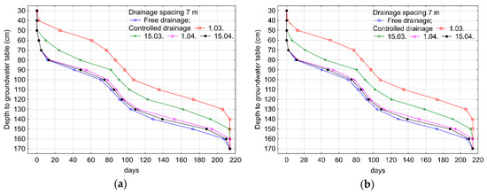
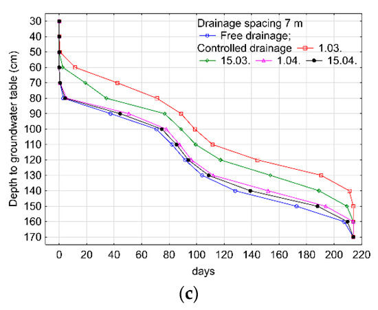
Figure 5.
Average duration of the groundwater depth in the case of free drainage (FD) and controlled drainage (CD) from a 7 m spacing drainage network, with the groundwater table at the beginning of simulation period of 40 (a), 60 (b), and 80 (c) cm b.s.l.
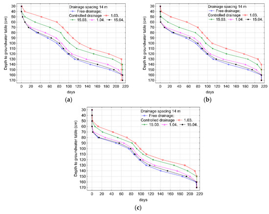
Figure 6.
Average duration of the groundwater depth in the case of free drainage (FD) and controlled drainage (CD) from a drainage network with 14 m spacing, with the groundwater table at the beginning of the simulation period of 40 (a), 60 (b), and 80 (c) cm b.s.l.
The initial conditions and the date of starting to block the outflow have the greatest impact on the groundwater table in the case of a drainage network with a spacing of 7 m and 14 m. Taking into account the outlet depth of the water level control structure (damming height) and the depth of the drainage system, it is possible to control the groundwater levels from of 50 cm b.s.l. to 90 cm b.s.l. Moreover, after heavy rainfall, groundwater levels may periodically exceed 50 cm b.s.l. Analysing the cumulative duration curves of the groundwater level depth horizontally, the greatest distances (impact) between the curve presenting the FD scenario and the curves for individual CD scenarios were obtained for levels from 60 to 90 cm b.s.l. In the case of groundwater levels ranging from 40 to 50 cm b.s.l., the impact of CD was at a lower level.
The average groundwater table in the period from March to September in the conventional drainage spacing of 7 and 14 m was 123 cm and 118 cm, respectively (Figure 7).
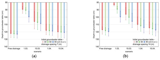
Figure 7.
Groundwater table in the various scenarios of the controlled drainage (CD) network compared to the conventional network (free drainage—FD) for 7 m (a) and 14 m (b) network spacing (bar charts with error bars show the average values, as well as the minimum and maximum values for the years 2014, 2017, and 2018).
The use of CD solutions at the beginning of blocking the outflow on 1 March may depend on the initial conditions. The groundwater table is stabilised at an average level of 88 to 99 cm b.s.l. and 86 to 95 cm b.s.l., respectively, for drainage spacing of 7 and 14 m. Moreover, when first blocking water in the drainage network on 15 March, the influence on the groundwater increase is visible. In other cases, the impact of CD on groundwater is at a lower level. The Kruskal–Wallis (K–W) and Dunn’s tests as post hoc procedures (p ≤ 0.05) showed that there were no significant differences between the average groundwater tables in the period from March to September and the FD and CD scenarios for 1 and 15 April. The influence of the initial groundwater table on the effectiveness of CD solutions in the case of drainage networks with a 7 m spacing decreases when delaying the blocking of the outflow on 15 March. On the other hand, in a drainage network with a spacing of 14 m, the impact of the initial conditions disappears on 1 April, which is confirmed by small differences between the successive scenarios. In the case of variants, assuming the outflow is blocked for 1 and 15 March, regardless of the initial conditions and the drainage network spacing, the impact of CD solutions on the depth of the groundwater level is visible throughout the whole period until September (upper part of Figure 8a,b). There are statistically significant differences between the average water tables for FD and CD. The differences in groundwater tables in relation to the conventional network are presented in Figure 8. It is clearly visible that, regardless of the initial conditions, starting to block the outflow on April 1 or 15 allows the groundwater to be raised by as much as 8 cm (lower part of Figure 8a,b).
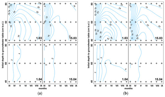
Figure 8.
Average increases in groundwater tables in successive months with different dates for blocking the outflow from the network with spacing of 7 m (a) and 14 m (b).
The use of CD solutions, apart from their influence on the groundwater table, also affects the sub-surface outflow from the drainage network. The duration of outflows was the same as the time of the groundwater’s table location above the drainage network level. Simulation calculations showed that outflows from the conventional network ranged from 28 to 63 mm and from 25 to 59 mm for spacings of 7 and 14 m, respectively (Figure 9). In the years 2014, 2017, and 2018, the weather conditions affected the average outflow from the network by ±5 mm. In the case of the groundwater table at the beginning of the simulation period at the level of 80 cm b.s.l., the outflow may be completely reduced. In CD scenarios with drain blocking on 1 or 15 March, the subsurface outflow can be reduced from 18 to 28 mm and from 18 to 25 mm, on average, from a drainage network with a spacing of 7 and 14 m, respectively. Taking into account the whole area of the analysed research object (107 ha), it is possible to retain about 19 ×·103 to 40·× 103 m3 of water in this way.
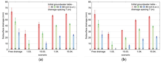
Figure 9.
Drainages from free drainage (FD) networks with 7 m (a) and 14 m (b) spacing and for different scenarios of controlled drainage (CD) (bar charts with error bars show the average values, as well as the minimum and maximum values for the years 2014, 2017, and 2018).
The relative impact of outflow blocking from the network is shown in Figure 10. The largest effects were achieved in scenarios in which outflow blocking started on 1 March. In the case of initial groundwater tables of 60 and 80 cm, outflows can be reduced from about 80% to 100%. If the date of blocking the outflow is delayed to 15 March, the reduction is lower. In the presented calculation scenarios, the influence of the initial groundwater table on the obtained results is clearly visible.
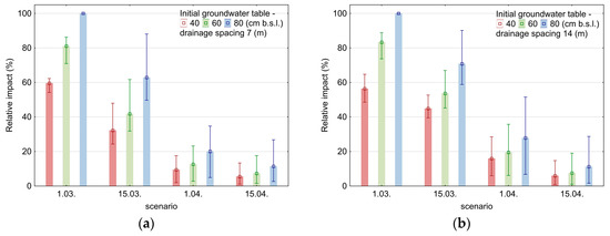
Figure 10.
The impact of CD solutions on drainage from drainage networks with 7 (a) and 14 m (b) spacing.
4. Discussion
The conducted research showed that CD solutions increase the groundwater table and reduce subsurface outflow from the drainage network. As a result, the water remains in the soil profile and can be available to the plants during their growing season. In the climatic conditions of Poland, it is important to start blocking the outflow from the network as early as possible. At the start date of blocking the outflow on 1 March, the reduction of the outflow from the network during the period from March to September was about 80% on average. With a delay in blocking the outflow, the impact of using CDs decreases and ranges from 8% to 50%. The results obtained in this study correspond to those obtained by other authors (Table 6).
Table 6.
The impact of CD on subsurface drainage compared to a free drainage (FD) system.
Relatively large differences in the results of the CD impact solutions on sub-surface outflow could result from different climatic conditions, soil properties, and technical parameters of the drainage network, i.e., drainage depth, spacing, and the height to which the outlet was raised [53]. Reduction of sub-surface outflows from fields is primarily of ecological significance, as it limits outflow of nitrate nitrogen. The reduction in the nitrate load with CD varied between 32% and 94% [20,51,52,54]. Wesström et al. [55] revealed no differences between nitrogen concentrations in subsurface drainage water from the free drainage and the control drainage networks. Nitrate losses tended to be lower in the controlled drainage than in the free drainage network, due to lower outflow. This is confirmed by the results of Ross et al. [56], which indicate that nitrate reductions are mainly due to reduced drainage outflow rather than enhanced denitrification. This is particularly important for Poland, where, in accordance with the requirements of the European Union, actions are taken to limit the outflow of N-NO3 from agricultural areas. These actions are aimed at improving the quality of surface waters and limiting their eutrophication. Ale et al. [51] suggested that the drain spacing and soil texture had a greater effect on nitrate load reduction than the cropping pattern. Furthermore, Golmohammadi et al. [30] suggest that the nitrate reduction to water bodies requires knowledge on different cropping management practices with CD.
From the point of view of the water needs of plants and the adaptation of agriculture to climate change, the impact of CD on groundwater regulation is more important. The obtained results indicate that CD allows the groundwater table to be increased, at the beginning of blocking the water outlet from 1 to 15 March, from 10 to 33 cm and from 10 to 41 for spacing of 7 and 14 m in relation to the free drainage system. If the blockade of water outflow is moved to April, the maximum water table can be increased by 13 cm. The obtained results show that with 7 and 14 m drainage spacing, and climatic conditions such as in central Europe, including Poland, a quick start in the blocking outflow from the drainage network in the period from 1 to 15 March is of key importance. In addition, this study shows that better CD effects were obtained for a drainage network, at the same drainage depth, with 14 m spacing. Darzi-Naftchali et al. [57] reported that shallow drains were more effective in controlling the water table compared with deep drains. Furthermore, Ale et al. [11] reported that the water table rose above the conventional drainage level during both the winter and the crop periods.
In the longer term, parallel field studies and further computer simulations should be carried out in order to adapt the CD practice to the water needs of plants and the field work dates. Attention should also be paid to the analysis of the remaining components of the water balance at the field scale. Research [33] shows that CD caused the reduction of subsurface drainage and indicates that these practices may increase surface runoff. Consequently, CD may cause soil erosion and water pollution with phosphorus [58,59].
This study shows that CD activities may contribute to the mitigation of the effects of climate change in Poland. Access to and proper use of technical infrastructure are the main factors influencing adaptation capabilities. Moreover, blocking the outflow of water from the drainage network facilitates the effective storage of water in the place of its greatest demand. These measures are more effective than the construction of retention reservoirs due to the need to distribute water over long distances and because of problems related to the eutrophication of water in reservoirs. In addition, the increase in retention contributes to the reduction of flood risk and the effects of drought. On the one hand, CD solutions allow one to retain water within the field and mitigate the effects of drought. On the other hand, they can help to reduce flooding. This is confirmed by the studies that showed that controlled drainage is an effective tool to reduce peak discharges and drought stress [16]. Moreover, Sunohara et al. [17] reported that the outflows exhibited lower peak flow rates from the CD solutions compared to the conventional drained network. Kulhavý and Fučík [60] indicate the need for policy makers to develop a global strategy for the use of drainage systems for sustainable agriculture. This confirms the importance of the research conducted in this study as a starting point for the adaptation of drainage systems to new climatic conditions. Future studies, apart from the impact of CD on groundwater depth and sub-surface runoff, should focus on other components of water balance, such as surface runoff, surface storage, and deep seepage, as well as the impact of water balance on potential crop yields.
5. Conclusions
On the basis of the conducted research, the following detailed conclusions were made:
- In the climatic conditions of central Poland, the best results related to the application of CD solutions are obtained at the beginning of operation in the period from 1 to 15 March.
- The solutions applied in the indicated time allow the groundwater table to be raised in relation to the free drainage network from 10 to 33 cm and from 10 to 41 in the case of spacing of 7 and 14 m.
- The application of CD solutions in small fields allows only for periodic maintenance of the assumed groundwater tables.
- The starting of blocking the outflow from the drainage network in the period from 1 to 15 March reduces the average outflow from the network by 50%–80%.
- Better effects related to the control of the outflow were obtained for a drainage network with a distance of 14 m.
- The influence of the initial groundwater table on the effectiveness of CD solutions in the case of drainage networks with 7 and 14 m spacing decreases with the delay of blocking the outflow on 15 March and 1 April, respectively.
Author Contributions
Conceptualization, M.S.; methodology, M.S. and M.K.; validation, M.S.; data preparation B.K. and M.K.; simulation M.K.; formal analysis, M.S. and M.K.; investigation, R.S., J.B., M.N., D.L., M.S., and B.K.; writing—original draft preparation, M.S., R.S. and M.K.; writing—review and editing, R.S., D.L., M.N., R.W. and M.K.; visualization, M.S., J.J., and R.W.; supervision, M.S.; project administration, M.S.; funding acquisition, M.S.
Funding
This research was funded by the Polish National Centre for Research and Development grant number BIOSTRATEG3/347837/11/NCBR/2017.
Acknowledgments
This study was done within the project “Technological innovations and system of monitoring, forecasting and planning of irrigation and drainage for precise water management on the scale of drainage/irrigation system (INOMEL)” under the BIOSTRATEG3 program, funded by the Polish National Centre for Research and Development. Contract No. BIOSTRATEG3/347837/11/NCBR/2017.
Conflicts of Interest
The authors declare no conflict of interest.
References
- EEA. Climate Change, Impacts and Vulnerability in Europe 2016-an IndicatorBased Report; EEA: Copenhagen, Denmark, 2017. [Google Scholar]
- Szwed, M.; Karg, G.; Pińskwar, I.; Radziejewski, M.; Graczyk, D.; Kędziora, A.; Kundzewicz, Z.W. Climate change and its effect on agriculture, water resources and human health sectors in Poland. Nat. Hazards Earth Syst. Sci. 2010, 10, 1725–1737. [Google Scholar] [CrossRef]
- Todeschini, S. Trends in long daily rainfall series of Lombardia (northern Italy) affecting urban stormwater control. Int. J Climatol. 2012, 32, 900–919. [Google Scholar] [CrossRef]
- Greve, P.; Orlowsky, B.; Mueller, B.; Sheffield, J.; Reichstein, M.; Seneviratne, S.I. Global assessment of trends in wetting and drying over land. Nat. Geosci. 2014, 7, 716. [Google Scholar] [CrossRef]
- Döll, P.; Jiménez-Cisneros, B.; Oki, T.; Arnell, N.W.; Benito, G.; Cogley, J.G.; Jiang, T.; Kundzewicz, Z.W.; Mwakalila, S.; Nishijima, A. Integrating risks of climate change into water management. Hydrol. Sci. J. 2015, 60, 4–13. [Google Scholar]
- Kundzewicz, Z.; Matczak, P. Extreme hydrological events and security. PIAHS 2015, 369, 181–187. [Google Scholar] [CrossRef]
- Kazak, J. The use of a decision support system for sustainable urbanization and thermal comfort in adaptation to climate change actions—The case of the Wrocław larger urban zone (Poland). Sustainability 2018, 10, 1083. [Google Scholar] [CrossRef]
- Szewrański, S.; Kazak, J.; Szkaradkiewicz, M.; Sasik, J. Flood risk factors in suburban area in the context of climate change adaptation policies–Case study of Wroclaw, Poland. J. Ecol. Eng. 2015, 16, 13–18. [Google Scholar] [CrossRef]
- Szewrański, S.; Chruściński, J.; van Hoof, J.; Kazak, J.; Świąder, M.; Tokarczyk-Dorociak, K.; Żmuda, R. A location intelligence system for the assessment of pluvial flooding risk and the identification of storm water pollutant sources from roads in suburbanised areas. Water 2018, 10, 746. [Google Scholar] [CrossRef]
- Iglesias, A.; Garrote, L. Adaptation strategies for agricultural water management under climate change in Europe. Agric. Water Manag. 2015, 155, 113–124. [Google Scholar] [CrossRef]
- Ale, S.; Bowling, L.C.; Brouder, S.M.; Frankenberger, J.R.; Youssef, M.A. Simulated effect of drainage water management operational strategy on hydrology and crop yield for Drummer soil in the Midwestern United States. Agric. Water Manag. 2009, 96, 653–665. [Google Scholar] [CrossRef]
- ICID. Agricultural Water Management for Sustainable Rural Development-Annual Report 2017–2018; ICID: New Delhi, India, 2018.
- Frankenberger, J.; Kladivko, E.; Sands, G.; Jaynes, D.; Fausey, N.; Helmers, M.; Brown, L. Drainage Water Management for the Midwest: Questions and Answers about Drainage Water Management for the Midwest; Purdue Extension: West Lafayette, IN, USA, 2006; 8p. [Google Scholar]
- Drury, C.F.; Tan, C.S.; Gaynor, J.D.; Oloya, T.O.; Welacky, T.W. Influence of controlled drainage-subirrigation on surface and tile drainage nitrate loss. J. Environ. Qual. 1996, 25, 317–324. [Google Scholar] [CrossRef]
- Jaynes, D.B. Changes in yield and nitrate losses from using drainage water management in central Iowa, United States. J. Soil Water Conserv. 2012, 67, 485–494. [Google Scholar] [CrossRef]
- Ritzema, H.P.; Stuyt, L.C.P.M. Land drainage strategies to cope with climate change in the Netherlands. Acta Agric. Scand. B Soil Plant Sci. 2015, 65, 80–92. [Google Scholar] [CrossRef]
- Sunohara, M.D.; Gottschall, N.; Craiovan, E.; Wilkes, G.; Topp, E.; Frey, S.K.; Lapen, D.R. Controlling tile drainage during the growing season in Eastern Canada to reduce nitrogen, phosphorus, and bacteria loading to surface water. Agric. Water Manag. 2016, 178, 159–170. [Google Scholar] [CrossRef]
- Gunn, K.M.; Fausey, N.R.; Shang, Y.; Shedekar, V.S.; Ghane, E.; Wahl, M.D.; Brown, L.C. Subsurface drainage volume reduction with drainage water management: Case studies in Ohio, USA. Agric. Water Manag. 2015, 149, 131–142. [Google Scholar] [CrossRef]
- Negm, L.M.; Youssef, M.A.; Jaynes, D.B. Evaluation of DRAINMOD-DSSAT simulated effects of controlled drainage on crop yield, water balance, and water quality for a corn-soybean cropping system in central Iowa. Agric. Water Manag. 2017, 187, 57–68. [Google Scholar] [CrossRef]
- Youssef, M.A.; Abdelbaki, A.M.; Negm, L.M.; Skaggs, R.W.; Thorp, K.R.; Jaynes, D.B. DRAINMOD-simulated performance of controlled drainage across the. Agric. Water Manag. 2018, 197, 54–66. [Google Scholar] [CrossRef]
- Skaggs, R.W. A Water Management Model for Shallow Water Table Soils; Water Resources Research Institute of the University of North Carolina: Raleigh, NC, USA, 1978. [Google Scholar]
- Breve, M.A.; Skaggs, R.W.; Parsons, J.E.; Gilliam, J.W. Using the DRAINMOD-N model to study effects of drainage system design and management on crop productivity, profitability and NO3–N losses in drainage water. Agric. Water Manag. 1998, 35, 227–243. [Google Scholar] [CrossRef]
- Youssef, M.A.; Skaggs, R.W.; Chescheir, G.M.; Gilliam, J.W. The nitrogen simulation model, DRAINMOD-N II. Trans. ASAE 2005, 48, 611–626. [Google Scholar] [CrossRef]
- Negm, L.M.; Youssef, M.A.; Skaggs, R.W.; Chescheir, G.M.; Jones, J. DRAINMOD–DSSAT model for simulating hydrology, soil carbon and nitrogen dynamics, and crop growth for drained crop land. Agric. Water Manag. 2014, 137, 30–45. [Google Scholar] [CrossRef]
- Skaggs, R.W. Field evaluation of a water management simulation model. Trans. ASAE 1982, 25, 666–674. [Google Scholar] [CrossRef]
- Gayle, G.A.; Skaggs, R.W.; Carter, C.E. Evaluation of a water management model for a Louisiana sugar cane field. J. Am. Soc. Sugar Cane Technol. 1985, 4, 18–28. [Google Scholar]
- Fouss, J.L.; Bengtson, R.L.; Carter, C.E. Simulating subsurface drainage in the lower Mississippi Valley with DRAINMOD. Trans. ASAE 1987, 30, 1679–1688. [Google Scholar] [CrossRef]
- Rogers, J.S. Water management model evaluation for shallow sandy soils. Trans. ASAE 1985, 28, 785–0790. [Google Scholar] [CrossRef]
- McMahon, P.C.; Mostaghimi, S.; Wright, F.S. Simulation of corn yield by a water management model for a coastal plain soil in Virginia. Trans. ASAE 1988, 31, 734–0742. [Google Scholar] [CrossRef]
- Golmohammadi, G.; Rudra, R.P.; Prasher, S.O.; Madani, A.; Goel, P.K.; Mohammadi, K. Modeling the impacts of tillage practices on water table depth, drain outflow and nitrogen losses using DRAINMOD. Comput. Electron. Agric. 2016, 124, 73–83. [Google Scholar] [CrossRef]
- Skaggs, R.W.; Youssef, M.A.; Gilliam, J.W.; Evans, R.O. Effect of controlled drainage on water and nitrogen balances in drained lands. Trans. ASABE 2010, 53, 1843–1850. [Google Scholar] [CrossRef]
- Skaggs, R.W.; Fausey, N.R.; Evans, R.O. Drainage water management. J. Soil Water Conserv. 2012, 67, 167A–172A. [Google Scholar] [CrossRef]
- Singh, R.; Helmers, M.J.; Crumpton, W.G.; Lemke, D.W. Predicting effects of drainage water management in Iowa’s subsurface drained landscapes. Agric. Water. Manag. 2007, 92, 162–170. [Google Scholar] [CrossRef]
- Sojka, M.; Jaskuła, J.; Wielgosz, I. Drought Risk Assessment in the Kopel River Basin. J. Ecol. Eng. 2017, 18, 134–141. [Google Scholar] [CrossRef]
- Iuss Working Group Wrb. World Reference Base for Soil Resources 2014, Update 2015: International Soil Classification System for Naming Soils and Creating Legends for Soil Maps. World Soil Resources Reports; FAO: Rome, Italy, 2015; No. 106. [Google Scholar]
- Thornthwaite, C.W. An approach toward a rational classification of climate. Geogr. Rev. 1948, 38, 55–94. [Google Scholar] [CrossRef]
- Van Schilfgaarde, J.; Bernstein, L.; Rhoades, J.D.; Rawlins, S.L. Irrigation management for salt control. J. Irrig. Drain. Eng. 1974, 100, 321–338. [Google Scholar]
- Kirkham, D. Theory of Land Drainage. In Drainage of Agricultural Lands; American Society of Agronomy: Madison, WI, USA, 1957. [Google Scholar]
- Skaggs, R.W. DRAINMOD Reference Report. Methods for Design and Evaluation of Drainage-Water Management Systems for Soils with High Water Tables; USDA-SCS, South National Technical Center: Fort Worth, TX, USA, 1980. [Google Scholar]
- Feddes, R.A.; Kabat, P.; Van Bakel, P.; Bronswijk, J.J.B.; Halbertsma, J. Modelling soil water dynamics in the unsaturated zone—State of the art. J. Hydrol. 1988, 100, 69–111. [Google Scholar] [CrossRef]
- Van Dam, J.C.; Huygen, J.; Wesseling, J.G.; Feddes, R.A.; Kabat, P.; Van Walsum, P.E.V.; Dan Diepen, C.A. Theory of SWAP Version 2.0; Simulation of Water Flow, Solute Transport and Plant Growth in the Soil-Water-Atmosphere-Plant Environment; DLO Winand Staring Centre: Wageningen, The Netherlands, 1997. [Google Scholar]
- Campbell, G.S.; Gee, G.W. Water potential: Miscellaneous methods. In Methods of Soil Analysis: Part 1—Physical and Mineralogical Methods; American Society of Agronomy: Madison, WI, USA, 1986. [Google Scholar]
- Klute, A. Water Retention: Laboratory Methods, Methods of Soil Analysis, Part I; Klute, A., Ed.; American Society of Agronomy: Madison, WI, USA, 1986; pp. 635–660. [Google Scholar]
- Van Genuchten, M.V.; Leij, F.J.; Yates, S.R. The RETC Code for Quantifying the Hydraulic Functions of Unsaturated Soils; Rep.EPA-600/2-91/065; U.S. Environ. Prot. Agency: Ada, OK, USA, 1991.
- Mualem, Y. A new model for predicting the hydraulic conductivity of unsaturated porous media. Water Resour. Res. 1976, 12, 513–522. [Google Scholar] [CrossRef]
- Klute, A.; Dirksen, C. Hydraulic Conductivity of Saturated Soils. In Methods of Soil Analysis; ASA and SSSA: Madison, WA, USA, 1986. [Google Scholar]
- Skaggs, R.W.; Youssef, M.A.; Chescheir, G.M. DRAINMOD: Model use, calibration, and validation. Trans. ASABE 2012, 55, 1509–1522. [Google Scholar] [CrossRef]
- Willmott, C.J. On the validation of models. Phys. Geogr. 1981, 2, 184–194. [Google Scholar] [CrossRef]
- Loague, K.; Green, R.E. Statistical and graphical methods for evaluating solute transport models: Overview and application. J. Contam. Hydrol. 1991, 7, 51–73. [Google Scholar] [CrossRef]
- Thorp, K.R.; Jaynes, D.B.; Malone, R.W. Simulating the long-term performance of drainage water management across the Midwestern United States. Trans. ASABE 2008, 51, 961–976. [Google Scholar] [CrossRef]
- Ale, S.; Bowling, L.C.; Owens, P.R.; Brouder, S.M.; Frankenberger, J.R. Development and application of a distributed modeling approach to assess the watershed-scale impact of drainage water management. Agric. Water Manag. 2012, 107, 23–33. [Google Scholar] [CrossRef]
- Wesström, I.; Messing, I.; Linner, H.; Lindström, J. Controlled drainage—Effects on drain outflow and water quality. Agric. Water Manag. 2001, 47, 85–100. [Google Scholar] [CrossRef]
- Williams, M.R.; King, K.W.; Fausey, N.R. Drainage water management effects on tile discharge and water quality. Agric. Water Manag. 2015, 148, 43–51. [Google Scholar] [CrossRef]
- Poole, C.A.; Skaggs, R.W.; Youssef, M.A.; Chescheir, G.M.; Crozier, C.R. Effect of drainage water management on nitrate nitrogen loss to tile drains in North Carolina. Trans. ASABE 2018, 61, 233–244. [Google Scholar] [CrossRef]
- Wesström, I.; Joel, A.; Messing, I. Controlled drainage and subirrigation—A water management option to reduce non-point source pollution from agricultural land. Agric. Ecosyst. Environ. 2014, 198, 74–82. [Google Scholar] [CrossRef]
- Ross, J.A.; Herbert, M.E.; Sowa, S.P.; Frankenberger, J.R.; King, K.W.; Christopher, S.F.; Yen, H. A synthesis and comparative evaluation of factors influencing the effectiveness of drainage water management. Agric. Water Manag. 2016, 178, 366–376. [Google Scholar] [CrossRef]
- Darzi-Naftchali, A.; Mirlatifi, S.M.; Shahnazari, A.; Ejlali, F.; Mahdian, M.H. Effect of subsurface drainage on water balance and water table in poorly drained paddy fields. Agric. Water Manag. 2013, 130, 61–68. [Google Scholar] [CrossRef]
- Halecki, W.; Kruk, E.; Ryczek, M. Evaluation of Soil Erosion in the Mątny Stream Catchment in the West Carpathians Using the G2 model. Catena 2018, 164, 116–124. [Google Scholar] [CrossRef]
- Halecki, W.; Kruk, E.; Ryczek, M. Predicting of nitrate nitrogen, total phosphorus fluxes and suspended sediment concentration (SSC) as an indicators of surface-erosion process using ANN (Artificial Neural Network) based on geomorphological parameters in mountainous catchments. Ecol. Indic. 2018, 91, 461–469. [Google Scholar] [CrossRef]
- Kulhavý, Z.; Fučík, P. Adaptation Options for Land Drainage Systems Towards Sustainable Agriculture and the Environment: A Czech Perspective. Pol. J. Environ. Stud. 2015, 24, 1085–1102. [Google Scholar] [CrossRef]


© 2019 by the authors. Licensee MDPI, Basel, Switzerland. This article is an open access article distributed under the terms and conditions of the Creative Commons Attribution (CC BY) license (http://creativecommons.org/licenses/by/4.0/).