Is the Current Trend of Income Inequality Sustainable?

Abstract

Rising income inequality has become a major concern for policymakers and academic researchers. Very high levels of income inequality may result in serious social, political, and economic problems. In this paper, I analyze the trend of Gini index, which is the most commonly used measure for income inequality, to see if the current trend is sustainable in the long run for OECD and major non-OECD countries. Specifically, I use autoregressive time series models to test the sustainability of income inequality. I first analyze the Gini index to see if the time series is stationary and has a steady-state value below 1. If the series has a unit root, I take the first difference and check if the first difference is stationary and has a 0 or negative steady-state value. Results show that while many countries show signs of sustainability, there are a few countries that do not.

1. Introduction

Rising income inequality has become a major concern for policymakers, economists, and other social scientists. According to the World Inequality Report 2018 [1], the top 10% earners’ share in the total national income in 2016 was 47% in US–Canada, 41% in China, and 37% in Europe. These figures have increased remarkably except for Europe. The increase in the top 1% earners’ share is more remarkable. In 1980, the share of the top 1% earners in national total income was about 11% in the United States; but in 2016, it was about 20% [1]. In contrast, the share of the bottom 50% earners in the United States was about 20% in 1980; but it is only about 13% in 2016 (Wealth is more concentrated at the top. In the United States, for example, the share of the top 1% wealth holders has increased from 22% in 1980 to 39% in 2014 [1]. In this paper, I focus on income inequality.).

The current trend of rising income inequality has put income distribution back in the major topic of economic research [2]. In the 1950s, Kuznets [3,4] predicted that as the economy grows, inequality will first rise in the early stage of industrialization and then eventually fall as the benefit of economic growth spreads more evenly to many people. Since then, the focus of economic research has shifted to the study of economic growth and business cycles. Unlike the prediction of Kuznets, the level of income inequality has not fallen back despite the rapid economic growth in the second half of the 20th century. Instead, it is continuously rising and has become a major social and political problem. Reflecting this trend, it is very natural that income distribution has gained the interest of academic researchers again. There has been a number of studies estimating the level of income inequality, especially since the pioneering work of Piketty and Saez [5], and studying causes and consequences of the rising income inequality [6,7].

Not only is rising income inequality a social and political problem, but it is also an economic problem. Conventional wisdom in economic theory tells that there is a trade-off between efficiency and equity [8]. In the current context, there is a trade-off between economic growth and income inequality. Inequality in rewards motivates people to work harder, invest more, innovate, and take risks, which are all helpful for economic growth. The efforts of governments to reduce the gap between the successful and the unsuccessful will discourage the incentives to work, invest, innovate, and take risks. So the question in the conventional economic theory is to find the balance between efficiency and equity. More recent studies, however, question the existence of the trade-off itself. In other words, there is a possibility and evidence that inequality is harmful, rather than helpful, to economic growth. For example, Berg and Ostry [9] find that growth spells are longer in countries where income is distributed more equally. In fact, the negative relationship between economic growth and income inequality is not new in the political–economy literature. Alesina and Rodrik [10] and Persson and Tabellini [11], for example, investigate the mechanism that inequality affects growth. According to their models, higher inequality calls for a higher level of taxation and redistribution, which adversely affects economic growth. So, in their models, it is the government policy, not the inequality per se, that negatively affects growth. However, a recent study shows that lower net (i.e., after taxes and transfers) inequality is associated with faster economic growth and that redistribution policies in many cases are helpful, not harmful, to economic growth [12,13]. Higher inequality, for example, hurts physical and human capital accumulation of children from low-income families [14]. Additionally, as stagnant or shrinking incomes of middle-class and poor households are often associated with high leverage and overextention of credit, the economy becomes more prone to financial crises [15,16]. Instead of discouraging economic incentives, government spending on education and health, for example, can increase employment and raise productivity of workers.

In fact, the size of government has increased a lot in many countries during the 20th century. Total public expenditure as a percentage of GDP was, on average, 35.0% in 1970 but 43.8% in 2005 [17]. The increase is more remarkable in some of the European countries. Total public expenditure increased from 39.2% to 53.9% of GDP in France between 1970 and 2005, from 38.4% to 46.8% in Germany, and from 43.9% to 56.3% in Sweden; while it increased from 32.3% to 39.3% in the United States [17]. The size of social expenditure shows a similar trend. Government expenditure on subsidies and transfers increased from 2.1% of GDP in 1937 to 11.0% in 1998 in the United States; and from 6.8% to 19.0% in European Union (the figure for EU is a simple average of ten EU countries (Austria, Belgium, France, Germany, Ireland, Italy, the Netherlands, Spain, and the United Kingdom)) over the same period [18]. More recent years, however, have shown less remarkable, or even a downward trend in the size of government. Some countries have reduced public spending (often referred to as “fiscal consolidation” or “austerity”) to curb rising public debt and, therefore, to prevent a fiscal crisis [19]. Some countries have also reduced tax burdens on corporations and capital income to prevent capital outflows toward other countries, especially, to tax havens [20].

Then, why is income inequality rising in the first place? There are a lot of studies on this topic and a few factors are usually mentioned. First, technological progress rewards high-skilled workers a lot more than low-skilled workers. In other words, skill premium has increased a lot during the past several decades, and those with much demanded but scarce skills (e.g., information technology, finance, etc.) have benefited the most. Second, globalization and financial deepening have also increased income disparity, but the effect is usually estimated to be smaller than the increase in skill premium. Third, changes in labor market institutions and government fiscal policies are also responsible for rising income inequality. Reforms toward more flexible labor markets can have intended benefits and at the same time weaken employment protection and bargaining power of low-skill workers. Additionally, in many countries, tax and transfer policies have become less progressive over the past several decades. Fourth, wealth is becoming more concentrated at the top, causing capital income, which is income from wealth, to be more unequally distributed. Furthermore, changing family structures also affect income inequality. The share of single-headed households is increasing and now the match between a high-earning man and a high-earning woman is increasingly common (so called “assortative mating”). Both of these factors worsen income inequality [7].

Income inequality is continuously rising, but very high levels of income inequality will not be politically and economically sustainable. If most of the national income is concentrated on a very small number of people or households, political pressure from the rest of the population will induce the government to take corrective actions. According to a well-known political economy model, rising income inequality makes the median voter (the median income earner) poorer relative to the mean income and, therefore, induces the median voter to voter for a higher tax rate [21]. Furthermore, very high levels of income inequality undermine domestic demand, because very rich people have a low propensity to consume and there will not be sufficient demand to pull the economy [22].

In this paper, I study the sustainability of income inequality. I use the Gini index, which is the most commonly used measure for income inequality, in my analysis. The Gini index ranges from 0 (complete equality) to 1 (complete inequality) and is based on the Lorenz curve that represents the cumulative distribution of income, i.e., the share of the total income earned by the bottom x (some share) of the population. The Gini index is defined as the ratio ${\displaystyle \frac{A}{A+B}}$ in Figure 1 [23]. If everyone has the same income, the Lorenz curve is the same as the 45 degree line, the area of A is zero, and the area of B is the entire triangle. In this case, the Gini index is zero. If one person has all the income, the Lorenz curve coincides with the horizontal axis for x < 1 and it is 1 at x = 1. Therefore, the area of A is the entire triangle and the area of B becomes zero. In this case, the Gini index becomes one.

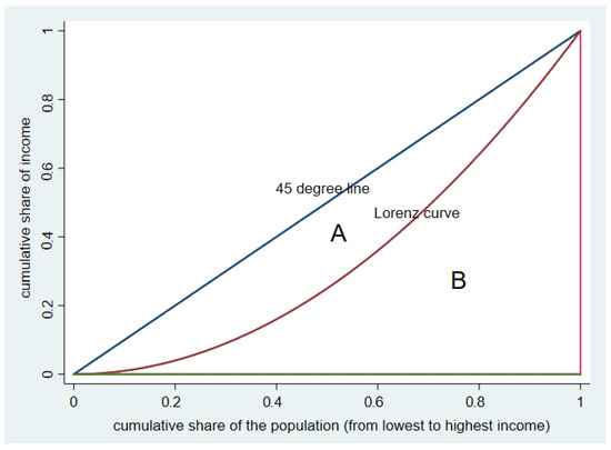
Figure 1. The Gini index.

Using the Gini index, I analyze the trend of income inequality to see if the current trend is sustainable in the long run for each of 36 OECD member countries and major non-OECD countries (Brazil, China, and Russia). Specifically, I use autoregressive time series analysis to check if the Gini coefficient series is stationary and converging to a value less than 1. If the Gini coeffcient has a unit root, I take the first difference of the Gini coefficient and see if the first difference is stationary and converging to 0 or a negative value. Time series analysis has been used to test, for example, the sustainability of fiscal policy ([24,25,26]), but, to the best of my knowledge, this is the first attempt to analyze the sustainability of income inequality using these statistical methods.

The rest of this paper is organized as follows. Section 2 explains the data used in the analysis and shows summary statistics. Section 3 explains empirical methodology and shows the results. Section 4 concludes the paper with a summary of the result and directions for future research.

2. Data and Summary Statistics

For empirical analyses, I use data from the Standardized World Income Inequality Database (SWIID) ([27]). The SWIID incorporates data from various sources including OECD, World Bank, Eurostat, United Nations, national statistical offices, and academic research to increase the comparability of income inequality statistics for a larger set of countries and a longer period of time than existing data sets. The Luxembourg Income Study (LIS) is served as the standard when computing the statistics. Currently, the SWIID covers 196 countries and as many years as possible from 1960 for each country. In this study, I use two indices—market income and disposable income Gini coefficients. Both measures are estimated using equivalized (square root scale) household income (In the SWIID dataset, the Gini estimates (and associated uncertainty) are represented by 100 draws from the posterior distribution. I use the mean of the 100 draws as the Gini coefficient for the country in the year.).

Table 1 shows the basic statistics for 36 OECD countries and 3 non-OECD major countries (Brazil, China, and Russia) that are comparable to OECD countries in the size of the economy. Specifically, it reports the first and latest years of data, the Gini coefficients for market income and disposable income in 2015 (2015 is the latest year in which there is no missing entry for every country in the sample) and the difference between the two for each country. The data cover years as far back as 1960 (Germany, Sweden, and Brazil) and as recent as 2018 (United Kingdom). The Gini coefficient for market income ranges from 0.339 (Korea) to 0.537 (Brazil). The Gini coefficient for disposable income ranges from 0.245 (Slovak Republic) to 0.451 (Mexico and Brazil). The difference between them, which is mainly the effect of the government’s fiscal policy, ranges from 0.018 (Mexico) to 0.241 (Sweden). While there is no distinctive pattern in the Gini coefficient of market income, there are some patterns in the Gini coefficient of disposable income and the difference between the two Gini coefficients. First, those with a low value of the Gini coefficient of disposable income are mostly European countries. Second, those with a large difference between the two Gini coefficients, which is a result of government’s redistribution policies, are also mostly European countries. Those with a small difference between the two are mainly countries in Latin America and Asia. Many European countries, in which market income is more equally distributed, have more generous welfare policies making disposable income even more equally distributed. In a sense, equality multiplies itself [28].

Table 1. Summary statistics.

Country			Gini Index in 2015
	Begin Year	End Year	Market Income	Disposable Income	Difference
Australia	1967	2016	0.480	0.331	0.149
Austria	1983	2017	0.486	0.283	0.203
Belgium	1979	2016	0.487	0.256	0.231
Canada	1969	2017	0.458	0.306	0.152
Chile	1968	2017	0.511	0.448	0.063
Czech Republic	1988	2016	0.445	0.250	0.195
Denmark	1976	2017	0.489	0.264	0.225
Estonia	1988	2016	0.487	0.331	0.156
Finland	1966	2017	0.478	0.252	0.225
France	1962	2016	0.488	0.297	0.191
Germany	1960	2016	0.522	0.291	0.230
Greece	1974	2016	0.514	0.337	0.177
Hungary	1962	2017	0.512	0.276	0.236
Iceland	1992	2015	0.372	0.249	0.123
Ireland	1973	2015	0.507	0.295	0.212
Israel	1979	2017	0.477	0.356	0.121
Italy	1967	2016	0.496	0.338	0.159
Japan	1961	2015	0.439	0.317	0.123
Korea	1965	2017	0.339	0.313	0.026
Latvia	1988	2017	0.478	0.350	0.127
Lithuania	1988	2016	0.531	0.352	0.179
Luxembourg	1985	2016	0.479	0.291	0.188
Mexico	1963	2016	0.468	0.451	0.018
Netherlands	1977	2016	0.478	0.271	0.207
New Zealand	1982	2017	0.478	0.329	0.148
Norway	1970	2017	0.449	0.257	0.192
Poland	1983	2016	0.490	0.303	0.188
Portugal	1968	2016	0.520	0.335	0.184
Slovak Republic	1988	2016	0.401	0.245	0.156
Slovenia	1987	2016	0.420	0.250	0.170
Spain	1974	2016	0.506	0.340	0.166
Sweden	1960	2017	0.499	0.258	0.241
Switzerland	1980	2015	0.408	0.291	0.117
Turkey	1987	2017	0.443	0.402	0.041
United Kingdom	1961	2018	0.523	0.330	0.193
United States	1961	2017	0.507	0.382	0.126
Brazil	1960	2017	0.537	0.451	0.086
China	1978	2015	0.471	0.412	0.059
Russia	1988	2016	0.445	0.335	0.110

Figure 2 and Figure 3, which are drawn using the data described above, show the evolution of the Gini coefficients for four countries: The largest economy in North America (United States); in Europe (Germany); in Scandinavia (Sweden) (Scandinavia is a part of Europe, but countries in Scandinavia are known for relatively equal distribution of income and generous welfare systems, so I include one countries from the area); and in Asia (China). The first figure is the Gini coefficient of market income and the second figure is that of disposable income. In the first figure, we see that the Gini coefficients in Germany and Sweden were decreasing until the early 1970s (Germany) and early 1980s (Sweden) and then began to increase, while that in the United States is continuouly rising. Although the absolute level of market income Gini coefficient is lower in China, it increases very fast. In the second figure, we see a similar pattern for disposable income inequality. The Gini coefficient of disposable income was initially decreasing and then began to rise in the early 1980s in Germany and Sweden, while it continuously rises in the United States. The Gini coefficient was rising very fast in China until the global financial crisis, since then, it has been decreasing, although there has been a revival in very recent years.

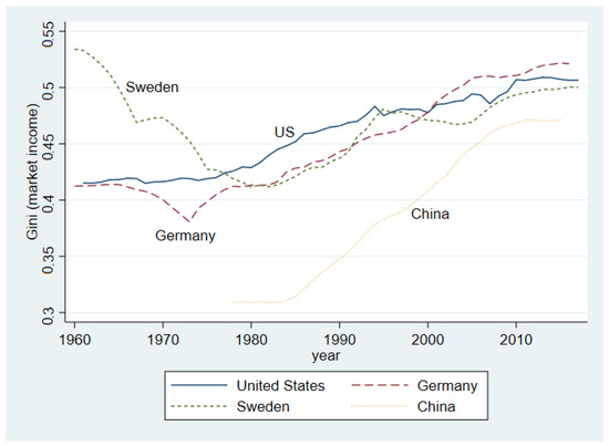
Figure 2. Gini coefficient (market income).

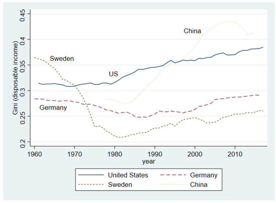
Figure 3. Gini coefficient (disposable income).

From the two figures above, we see that different countries have a difference level of the Gini coefficient and a different trend. So, in the next section, I analyze the trend of the income inequality for each of the 36 OECD countries and 3 non-OECD major countries (Brazil, China, and Russia).

3. Empirical Methodology and Results

In this section, I show the results from autoregressive time series analysis. The current value of a time series variable may depend on the past, or lagged values of the same variable. In general, an autoregressive model of order p (i.e., $AR\left(p\right)$ model) is defined as the following equation:

$$y_t={\alpha }_0+\sum _{i=1}^p{\alpha }_i·y_{t-i}+{ϵ}_t,$$

where ${\alpha }_0$ is a constant and ${ϵ}_t$ is assumed to be white noise. A critical question in this model is how many lags we should include in the estimation. Before I present a formal test of determining the number of lags, i.e., the value of p, I show the results of $AR\left(5\right)$ models for several countries in Table 2. For each country, I run two regressions—one with market income Gini coefficients and the other with disposable income Gini coefficients. We can see that in most of the cases, only the value of the immediate past ($y_{t-1}$) is statistically significant.

Table 2. Autoregressive models of order 5 ($AR\left(5\right)$).

	United States		Germany		Sweden		China
	Market	Disposable	Market	Disposable	Market	Disposable	Market	Disposable
	Income	Income	Income	Income	Income	Income	Income	Income
$y_{t-1}$	0.957 ***	1.117 ***	1.514 ***	1.294 ***	1.554 ***	1.336 ***	1.756 ***	1.634 ***
	(0.147)	(0.146)	(0.148)	(0.146)	(0.145)	(0.145)	(0.177)	(0.186)
$y_{t-2}$	0.040	−0.128	−0.374	−0.174	−0.447	−0.259	−0.807 **	−0.648
	(0.203)	(0.219)	(0.268)	(0.240)	(0.268)	(0.244)	(0.354)	(0.421)
$y_{t-3}$	0.003	−0.033	−0.213	−0.086	−0.073	−0.072	−0.002	−0.077
	(0.203)	(0.219)	(0.272)	(0.240)	(0.276)	(0.247)	(0.363)	(0.584)
$y_{t-4}$	0.076	0.198	0.008	0.090	−0.142	0.028	0.120	0.173
	(0.203)	(0.217)	(0.269)	(0.239)	(0.267)	(0.244)	(0.342)	(0.565)
$y_{t-5}$	−0.083	−0.153	0.068	−0.158	0.075	−0.086	−0.079	−0.110
	(0.152)	(0.146)	(0.152)	(0.147)	(0.141)	(0.135)	(0.180)	(0.274)
constant	0.005	0.0005	−0.0003	0.009	0.016	0.013 ***	0.006 **	0.011 **
	(0.007)	(0.005)	(0.005)	(0.007)	(0.010)	(0.005)	(0.003)	(0.005)

Note: ***, ** represent the statistical significance at the 1%, 5% level, respectively.

The lag length in autoregressive models is usually determined by two criteria: the Akaike information criterion (AIC) and the Bayesian information criterion (BIC). There are both advantages and disadvantages from adding additional lagged variables. The advantage is that the model has better explanatory power, in other words, it reduces the sum of squared residuals (SSR). The disadvantage is that adding more lagged variables increases uncertainty in the estimation of parameters. AIC and BIC balance these two opposing forces and we select the number of lags which minimize the AIC or the BIC. Specifically, definitions of the AIC and the BIC are as follows [29]:

$$AIC\left(p\right)=ln{\displaystyle \frac{SSR\left(p\right)}{T}}+(p+1){\displaystyle \frac{2}{T}},$$

$$BIC\left(p\right)=ln{\displaystyle \frac{SSR\left(p\right)}{T}}+(p+1){\displaystyle \frac{lnT}{T}},$$

where T is the total number of periods and p is the number of lags included in the model.

Table 3 shows the test results for the United States. The first four columns are results from the analysis using the entire period and the last four columns are results from the analysis using periods since 1990. In each case, I test the market income Gini coefficient and the disposable income Gini coefficient separately. We see that in all cases, the AR(1) model has the lowest AIC and BIC. The same results hold for most of the other countries as well.

Table 3. Tests for determining the number of lags (United States).

	Entire Period				Since 1990
	Market		Disposable		Market		Disposable
p	AIC	BIC	AIC	BIC	AIC	BIC	AIC	BIC
1	−475.8	−471.7	−500.8	−496.8	−217.3	−214.7	−233.5	−230.9
2	−464.6	−458.6	−499.4	−493.3	−206.9	−203.1	−232.4	−228.6
3	−453.1	−445.2	−491.8	−483.9	−196.3	−191.5	−226.5	−221.6
4	−441.6	−431.7	−481.0	−471.2	−186.3	−180.4	−216.1	−210.2
5	−430.6	−418.9	−469.9	−458.2	−178.7	−171.8	−210.9	−204.1

So, in the main analysis, I use AR(1) models for each country. Specifically, I run the following regressions:

$$y_t={\alpha }_0+{\alpha }_1·y_{t-1}+{ϵ}_t,$$

where $y_t$ is a Gini coefficient in year t. I assume that the error term is a white noise with mean of zero and variance ${\sigma }^2$, i.e., ${ϵ}_t\sim WN(0,{\sigma }^2)$. Before presenting the main results, there are a couple of concerns. First, I check whether there is a high degree of serial correlation in the AR(1) error terms. Table 4 shows the autocorrelation of the residuals after running the AR(1) model for the United States. I run two separate regression—one for market income and the other for disposable income Gini coefficients. In both cases, the autocorrelation of the residuals is not high. So, the degree of serial correlation in the error term is not likely to be very high.

Table 4. Autocorrelation of residuals from the AR(1) process (United States).

	Market Income				Disposable Income
Lag	AC	PAC	Q	Prob > Q	AC	PAC	Q	Prob > Q
1	−0.0390	−0.0392	0.08961	0.7647	0.1048	0.1050	0.64864	0.4206
2	0.0008	−0.0014	0.08965	0.9562	0.0009	−0.0106	0.64869	0.7230
3	0.0005	−0.0003	0.08966	0.9930	−0.0320	−0.0311	0.71137	0.8705
4	0.0738	0.0751	0.43	0.9799	0.1345	0.1454	1.8416	0.7649
5	0.1602	0.1748	2.0641	0.8402	0.0452	0.0156	1.9716	0.8531
6	−0.2376	−0.2344	5.7328	0.4538	−0.0533	−0.0593	2.1558	0.9048
7	0.1568	0.1496	7.3635	0.3920	−0.0454	−0.0140	2.2927	0.9419
8	0.1232	0.1733	8.3906	0.3963	0.1848	0.2044	4.6044	0.7989
9	0.0303	0.0157	8.454	0.4891	−0.0114	−0.0686	4.6133	0.8666
10	−0.1847	−0.2432	10.862	0.3684	−0.0236	−0.0091	4.6525	0.9132

A more serious concern is the existence of a unit root. In the above equation, the absolute value of ${\alpha }_1$ should be less than 1 for the process to be stable. If the process has a unit root, which occurs when ${\alpha }_1$ is equal to 1, the process is not stationary (If it is larger than 1, the path will be explosive and, therefore, not stationary. If ${\alpha }_1$ is equal to 1 in the AR(1) process, it is called a random walk. (with or without a drift depending on whether there is a constant term ${\alpha }_0$.)). When an autoregressive model has a unit root, there exists a stochastic trend. The current value has a permanent effect on the future values and this effect makes forecasting very difficult. Moreover, when there is a unit root, t-values from the OLS regressions have a nonstandard distributions, making inference very difficult [29]. So, it is important to check whether a time series has a unit root, and if so, one should make the series stationary by taking first differences. Table 5 shows autocorrelation and partial autocorrelation of the Gini coefficients for the United States. For a stationary process, the autocorrelation usually disappears quickly, but not for a non-stationary process. In the table, we see that the autocorrelation persists very long for both market income and disposable income Gini coefficients. This implies that there may be a unit root in the processes. So, in the main analysis, I first test whether there is a unit root for each country and if so, I run the AR(1) model using first differences for that country.

Table 5. Autocorrelation of the Gini coefficients (United States).

	Market Income				Disposable Income
Lag	AC	PAC	Q	Prob > Q	AC	PAC	Q	Prob > Q
1	0.9613	0.9979	55.495	0.0000	0.9606	1.0098	55.416	0.0000
2	0.9206	0.0381	107.32	0.0000	0.9187	−0.1092	107.03	0.0000
3	0.8776	−0.0007	155.28	0.0000	0.8756	0.0069	154.77	0.0000
4	0.8324	−0.0021	199.25	0.0000	0.8308	0.0264	198.57	0.0000
5	0.7839	−0.0831	238.99	0.0000	0.7859	−0.1535	238.51	0.0000
6	0.7333	−0.1920	274.45	0.0000	0.7370	−0.0281	274.33	0.0000
7	0.6834	0.2233	305.87	0.0000	0.6883	0.0471	306.19	0.0000
8	0.6260	−0.1833	332.76	0.0000	0.6417	0.0032	334.45	0.0000
9	0.5737	−0.2061	355.82	0.0000	0.5919	−0.2241	359	0.0000
10	0.5220	−0.0539	375.31	0.0000	0.5399	0.0386	379.86	0.0000

In $AR\left(1\right)$ models ($y_t={\alpha }_0+{\alpha }_1·y_{t-1}+{ϵ}_t$), we can see whether the variable converges to a finite value in the long run. Specifically, If we add recursively, with $y_0$ given, we can see that

$$y_t=(1+{\alpha }_1+{\alpha }_1^2+{\alpha }_1^3+\dots +{\alpha }_1^{t-1})·{\alpha }_0+{\alpha }_1^t·y_0+\sum _{s=0}^{t-1}{\alpha }_1^s·{ϵ}_{t-s}.$$

With $0<{\alpha }_1<1$, the expectation of $y_t$ converges to $\frac{{\alpha }_0}{1-{\alpha }_1}$ in the limit as $t⟶\infty$, but if $\alpha >1$, it diverges.

I run the AR(1) regression for each of the OECD countries and a few non-OECD major countries (Brazil, China, and Russia). I first run the regression for the entire period in the data. Then, to have more comparable and relevant results, I also run the regression using more recent data (since 1990). I run the same regression separately for market income and disposable income Gini coefficients. I first check whether there is a unit root using the augmented Dicky–Fuller test [30]. In the AR(1) process ($y_t={\alpha }_0+{\alpha }_1·y_{t-1}+{ϵ}_t$), there is a unit root if ${\alpha }_1$ is equal to 1. Then, the process has a stochastic trend and a shock has a permanent impact on the series. If ${\alpha }_1$ is larger than 1, the process has an explosive trajectory. For the series to be stationary and for the inference to make sense, the process should have a nonexplosive trajectory. This occurs when ${\alpha }_1$ is less than 1. So, the null hypothesis of the unit root test is $H_0:{\alpha }_1=1$ and the alternative hypothesis is $H_1:{\alpha }_1<1$ (In a Dickey–Fuller test, we subtract $y_{t-1}$ from both sides of the equation (so the new equation becomes $△y_t={\alpha }_0+\beta ·y_{t-1}+{ϵ}_t$, where $\beta ={\alpha }_1-1$) and test whether the coefficient ($\beta ={\alpha }_1-1$) is equal to 0 or less than 0.). If the series does not have a unit root, I calculate the long-run convergent value of the series ($\frac{{\alpha }_0}{1-{\alpha }_1}$). If the long-run value is less than 1, I call the series sustainable. Table 6 shows the results from the regressions with market income Gini coefficients. We can see that while there are countries in which the income is stationary and the long-run steady-state value is less than 1, there are many other countries in which the Gini coefficient has a unit root and, therefore, is not stationary.

Table 6. AR(1) results of the Gini coefficients (market income).

	Entire Period			Since 1990
Country	Unit Root?	${\displaystyle \frac{{\mathit{\alpha }}_{\mathbf{0}}}{\mathbf{1}-{\mathit{\alpha }}_{\mathbf{1}}}}$	Sustainable?	Unit Root?	${\displaystyle \frac{{\mathit{\alpha }}_{\mathbf{0}}}{\mathbf{1}-{\mathit{\alpha }}_{\mathbf{1}}}}$	Sustainable?
Australia	Yes	-	-	No **	0.484	Yes
Austria	Yes	-	-	Yes	-	-
Belgium	Yes	-	-	No *	0.492	Yes
Canada	Yes	-	-	No **	0.462	Yes
Chile	Yes	-	-	Yes	-	-
Czech Republic	No ***	0.455	Yes	Yes	-	-
Denmark	Yes	-	-	Yes	-	-
Estonia	No **	0.492	Yes	No **	0.491	Yes
Finland	Yes	-	-	No ***	0.485	Yes
France	Yes	-	-	Yes	-	-
Germany	Yes	-	-	Yes	-	-
Greece	Yes	-	-	Yes	-	-
Hungary	Yes	-	-	No **	0.513	Yes
Iceland	Yes	-	-	Yes	-	-
Ireland	Yes	-	-	Yes	-	-
Israel	Yes	-	-	Yes	-	-
Italy	Yes	-	-	No ***	0.499	Yes
Japan	Yes	-	-	Yes	-	-
Korea	Yes	-	-	Yes	-	-
Latvia	No *	0.499	Yes	No **	0.493	Yes
Lithuania	No ***	0.549	Yes	No **	0.540	Yes
Luxembourg	Yes	-	-	No *	0.579	Yes
Mexico	Yes	-	-	Yes	-	-
Netherlands	Yes	-	-	Yes	-	-
New Zealand	Yes	-	-	No *	0.479	Yes
Norway	Yes	-	-	Yes	-	-
Poland	Yes	-	-	No ***	0.502	Yes
Portugal	No **	0.524	Yes	Yes	-	-
Slovak Republic	No**	0.426	Yes	Yes	-	-
Slovenia	Yes	-	-	Yes	-	-
Spain	Yes	-	-	Yes	-	-
Sweden	Yes	-	-	Yes	-	-
Switzerland	Yes	-	-	Yes	-	-
Turkey	Yes	-	-	Yes	-	-
United Kingdom	Yes	-	-	No ***	0.527	Yes
United States	Yes	-	-	Yes	-	-
Brazil	Yes	-		Yes	-	-
China	Yes	-	-	Yes	-	-
Russia	No ***	0.473	Yes	No ***	0.469	Yes

Note: No ***, No **, No * indicate that the null hypothesis of a unit root can be rejected at the 1%, 5%, and 10%, respectively; and Yes indicates that the null hypothesis of a unit root cannot be rejected at the 10% level.

People (and families) pay taxes and receive transfers depending on their economic circumstances. So, what actually matters is not market income but disposable income, which is market income minus net taxes (taxes minus transfers). As we see in the basic statistics table, the disposable income Gini coefficient differs greatly from the market income Gini coefficient in some countries (such as Sweden and Hungary), but the difference is negligible in other countries (such as Mexico and Korea).

Table 7 shows the results from the regressions with disposable income Gini coefficients. Where there are countries that show signs of sustainability in both market income and disposable income Gini coefficients, there are some countries showing signs of sustainability only in one of them.

Table 7. AR(1) results of the Gini coefficients (disposable income).

	Entire Period			Since 1990
Country	Unit Root?	${\displaystyle \frac{{\mathit{\alpha }}_{\mathbf{0}}}{\mathbf{1}-{\mathit{\alpha }}_{\mathbf{1}}}}$	Sustainable?	Unit Root?	${\displaystyle \frac{{\mathit{\alpha }}_{\mathbf{0}}}{\mathbf{1}-{\mathit{\alpha }}_{\mathbf{1}}}}$	Sustainable?
Australia	Yes	-	-	Yes	-	-
Austria	Yes	-	-	Yes	-	-
Belgium	Yes	-	-	No *	0.261	Yes
Canada	Yes	-	-	No *	0.308	Yes
Chile	Yes	-	-	Yes	-	-
Czech Republic	No **	0.258	Yes	No **	0.254	Yes
Denmark	Yes	-	-	Yes	-	-
Estonia	No **	0.343	Yes	No *	0.342	Yes
Finland	Yes	-	-	No *	0.262	Yes
France	Yes	-	-	Yes	-	-
Germany	Yes	-	-	Yes	-	-
Greece	No *	0.333	Yes	Yes	-	-
Hungary	Yes	-	-	Yes	-	-
Iceland	Yes	-	-	Yes	-	-
Ireland	Yes	-	-	Yes	-	-
Israel	Yes	-	-	No *	0.366	Yes
Italy	Yes	-	-	No ***	0.334	Yes
Japan	Yes	-	-	Yes	-	-
Korea	Yes	-	-	Yes	-	-
Latvia	No **	0.379	Yes	No **	0.368	Yes
Lithuania	No *	0.362	Yes	Yes	-	-
Luxembourg	Yes	-	-	Yes	-	-
Mexico	Yes	-	-	Yes	-	-
Netherlands	Yes	-	-	Yes	-	-
New Zealand	Yes	-	-	Yes	-	-
Norway	Yes	-	-	Yes	-	-
Poland	Yes	-	-	No ***	0.311	Yes
Portugal	No *	0.338	Yes	Yes	-	-
Slovak Republic	No **	0.264	Yes	No **	0.259	Yes
Slovenia	Yes	-	-	Yes	-	-
Spain	Yes	-	-	Yes	-	-
Sweden	No *	0.228	Yes	Yes	-	-
Switzerland	Yes	-	-	No *	0.286	Yes
Turkey	Yes	-	-	Yes	-	-
United Kingdom	Yes	-	-	Yes	-	-
United States	Yes	-	-	Yes	-	-
Brazil	Yes	-	-	Yes	-	-
China	Yes	-	-	Yes	-	-
Russia	No ***	0.363	Yes	No ***	0.361	Yes

Note: No ***, No **, No * indicate that the null hypothesis of a unit root can be rejected at the 1%, 5%, and 10%, respectively; and Yes indicates that the null hypothesis of a unit root cannot be rejected at the 10% level.

In both cases (market income and disposable income), the number of countries with unsustainable income inequality is reduced when we restrict the sample to more recent periods. It could be that while the absolute level of income inequality is still increasing, the speed of increase is reduced due to the market’s self-correcting mechanism or the government’s efforts. It could also be that when we reduce the sample period, the period after the global financial crisis, during which income inequality has been reducing or increasing at a lower rate, takes a larger portion of the sample. In any case, it requires further analysis in the future.

In many countries, there is a unit root in the AR(1) process for the Gini coefficient. The standard remedy is to take first differences on the original data to make the process stationary. Table 8 shows autocorrelation of the first differences in the Gini coefficient. Unlike the autocorrelation in the Gini coefficient, the autocorrelation disappears quickly for the first differences in the Gini coefficient. So, it seems very probable that the AR(1) process for the first differences in the Gini coefficient does not have a unit root.

Table 8. Autocorrelation of the first differences in the Gini coefficients (United States).

	Market Income				Disposable Income
Lag	AC	PAC	Q	Prob > Q	AC	PAC	Q	Prob > Q
1	−0.0407	−0.0409	0.09776	0.7545	0.1190	0.1195	0.83563	0.3607
2	−0.0012	−0.0035	0.09785	0.9523	0.0179	0.0038	0.85483	0.6522
3	−0.0020	−0.0032	0.0981	0.9921	−0.0142	−0.0158	0.86713	0.8334
4	0.0713	0.0725	0.41581	0.9812	0.1471	0.1568	2.2183	0.6957
5	0.1578	0.1732	2.0023	0.8488	0.0592	0.0271	2.4412	0.7853
6	−0.2404	−0.2372	5.7576	0.4509	−0.0410	−0.0492	2.5506	0.8628
7	0.1552	0.1481	7.3552	0.3929	−0.0419	−0.0093	2.6671	0.9140
8	0.1231	0.1730	8.3811	0.3972	0.1827	0.2085	4.9261	0.7654
9	0.0308	0.0151	8.4466	0.4898	−0.0088	−0.0583	4.9314	0.8402
10	−0.1836	−0.2434	10.826	0.3713	−0.0129	0.0076	4.9432	0.8949

For those countries that have a unit root in the AR(1) process for the Gini coefficient, I run the following regression of the first differences:

$$△y_t={\alpha }_0+{\alpha }_1·△y_{t-1}+{ϵ}_t,$$

where $y_t$ is a Gini coefficient in year t and $△y_t=y_t-y_{t-1}$. The assumptions about the error term are the same as in the AR(1) process for the Gini coefficient. Before the main analysis, I show, in Table 9, the residuals after running the regression for the United States. We can see from the table that residuals are not serially correlated. So, the degree of serial correlation in the error term is not likely to be high.

Table 9. Autocorrelation of residuals from the AR(1) process (United States).

	Market Income				Disposable Income
Lag	AC	PAC	Q	Prob > Q	AC	PAC	Q	Prob > Q
1	−0.0024	−0.0024	0.00033	0.9856	−0.0022	−0.0022	0.00028	0.9867
2	−0.0026	−0.0028	0.00074	0.9996	−0.0079	−0.0079	0.00393	0.9980
3	−0.0041	−0.0048	0.00173	1.0000	−0.0418	−0.0422	0.10929	0.9907
4	0.0763	0.0786	0.35923	0.9857	0.1215	0.1235	1.0164	0.9073
5	0.1459	0.1551	1.694	0.8896	0.0238	0.0251	1.052	0.9583
6	−0.2472	−0.2557	5.6031	0.4691	−0.0896	−0.0866	1.5656	0.9550
7	0.1483	0.1604	7.0401	0.4247	−0.0743	−0.0671	1.926	0.9638
8	0.1278	0.1615	8.1292	0.4209	0.1915	0.1981	4.372	0.8221
9	0.0266	−0.0069	8.1773	0.5164	−0.0168	−0.0277	4.3912	0.8838
10	−0.1814	−0.2354	10.469	0.4004	−0.0294	−0.0163	4.4515	0.9247

In this analysis, for the first differences in the Gini coefficient, I use a different criterion for sustainability. If the process is stationary and the value of ${\alpha }_0$ is 0 or negative, the long-run steady-state value of $△y$ will be 0 or negative so that the Gini coefficient does not continuously increase. Therefore, it is probable that those countries have a sustainable trend of income inequality. Table 10 and Table 11 show the result—one for market income and the other for disposable income Gini coefficients. Now, there are many countries for which the AR(1) process for the Gini coefficient has a unit root but for the first difference is stationary and have a negative or statistically insignificant constant (${\alpha }_0$). Still, there are countries in which the first difference has a unit root. In the analysis of the first differences in the Gini coefficient of disposable income (entire period), for example, Korea has a unit root. For the countries that have a unit root in the first difference of the Gini coefficient, not only their Gini coefficients but also the first differences of them are nonstationary. The first differences have a stochastic trend and are explosive. So, income inequality in these countries are very unlikely to be stable. There are also countries (e.g., the United States) that do not have a unit root in the first difference but the value of ${\alpha }_0$ is positive and statistically significant. In such countries, the first difference in the Gini coefficient is positive, which means that the Gini coefficient is continuously rising. This could be a sign of unsustainable income inequality.

Table 10. AR(1) results of the first difference in the Gini coefficients (market income).

	Entire Period		Since 1990
Country	Unit Root?	${\mathit{\alpha }}_{\mathbf{0}}$	Unit Root?	${\mathit{\alpha }}_{\mathbf{0}}$
Australia	No *	0.001 **	·	·
Austria	Yes	-	No*	0.0008
Belgium	Yes	-	·	·
Canada	No ***	0.001	·	·
Chile	No ***	0.00002	No ***	−0.0003
Czech Republic	·	·	Yes	-
Denmark	No **	0.001 *	No ***	0.002 **
Estonia	·	·	·	·
Finland	Yes	-	·	·
France	No **	0.0002	Yes	-
Germany	No **	0.0009 *	Yes	-
Greece	Yes	-	Yes	-
Hungary	Yes	-	·	·
Iceland	Yes	-	Yes	-
Ireland	No **	0.0005	No **	0.0002
Israel	Yes	-	Yes	-
Italy	Yes	-	·	·
Japan	No *	0.0007 **	Yes	-
Korea	Yes	-	No *	0.0009*
Latvia	·	·	·	·
Lithuania	·	·	·	·
Luxembourg	No **	0.002 ***	·	·
Mexico	Yes	-	Yes	-
Netherlands	No ***	0.0006	Yes	-
New Zealand	Yes	-	·	·
Norway	No *	0.0002	No*	0.002
Poland	No *	0.001	·	·
Portugal	·	·	No **	−0.0002
Slovak Republic	·	·	No **	0.0002
Slovenia	Yes	-	Yes	-
Spain	No *	0.0007	Yes	-
Sweden	Yes	-	Yes	-
Switzerland	No *	0.0002	Yes	-
Turkey	No **	−0.0003	No **	−0.0005
United Kingdom	No **	0.0008	·	·
United States	No ***	0.002 ***	No ***	0.002 *
Brazil	No **	−0.0004	Yes	-
China	Yes	-	Yes	-
Russia	·	·	·	·

Note: ***, **, and * represent the statistical significance at the 1%, 5%, and 10%, respectively. Counties marked with “·” are the ones in which the Gini coefficient does not have a unit root in the previous analysis.

Table 11. AR(1) results of the first difference in the Gini coefficients (disposable income).

	Entire Period		Since 1990
Country	Unit Root?	${\mathit{\alpha }}_{\mathbf{0}}$	Unit Root?	${\mathit{\alpha }}_{\mathbf{0}}$
Australia	No ***	0.0008	No **	0.001 *
Austria	No **	0.0006	No **	0.0004
Belgium	No **	0.0003	·	·
Canada	No **	−0.0002	·	·
Chile	Yes	-	Yes	-
Czech Republic	·	·	·	·
Denmark	No ***	0.0006	No **	0.001 *
Estonia	·	·	·	·
Finland	No *	0.0002	·	·
France	No *	0.0002	Yes	-
Germany	No **	0.00007	Yes	-
Greece	·	·	No *	−0.0002
Hungary	No *	0.0002	Yes *	0.0001
Iceland	Yes	-	Yes	-
Ireland	No *	−0.00004	No *	−0.0006
Israel	Yes	-	·	·
Italy	No *	−0.0005	·	·
Japan	No **	0.0005	No *	0.0005
Korea	Yes	-	Yes	-
Latvia	·	·	·	·
Lithuania	·	·	No**	0.001
Luxembourg	No ***	0.002 ***	No ***	0.002 ***
Mexico	No *	−0.0006 *	No *	−0.0005
Netherlands	No **	0.0004	Yes	-
New Zealand	Yes	-	Yes	-
Norway	No **	−0.0001	No *	0.0008
Poland	No *	0.0007	·	·
Portugal	·	·	Yes	-
Slovak Republic	·	·	·	·
Slovenia	No **	0.0006	No **	0.0004
Spain	No **	0.0001	Yes	-
Sweden	·	·	No*	0.001*
Switzerland	No *	−0.0002	·	·
Turkey	Yes	-	Yes	-
United Kingdom	Yes	-	No **	−0.0002
United States	No ***	0.001 ***	No ***	0.002 ***
Brazil	No *	−0.0001	Yes	-
China	Yes	0.0008	Yes	-
Russia	·	·	·	·

Note: ***, **, and * represent the statistical significance at the 1%, 5%, and 10%, respectively. Counties marked with “·” are the ones in which the Gini coefficient does not have a unit root in the previous analysis.

4. Conclusions

In this paper, I analyze whether the current trend of income inequality is sustainable in OECD and non-OECD major countries. I judge the sustainability of income inequality from autoregressvie time series analyses. If the time series of the Gini coefficient is stationary and has a long-run steady-state value below 1, the current trend of income inequality seems sustainable. If the Gini coefficient has a unit root, I take the first differences and check if the first difference is stationary and has a 0 or negative long-run steady-state value. If so, it is probable that the income inequality is sustainable. While many countries show signs of sustainability, there are some countries that do not. There are also some interesting cases even within the same country. Some countries exhibit signs of sustainability only in the reduced sample (since 1990) but not in the entire sample and vice versa. Similarly, some countries exhibit signs of sustainability in disposable income but not in market income and vice versa. In addition to between-country comparisons, such within-country comparison may give important implications on the trend of income inequality and associated policy issues.

Rising income inequality is a major concern for researchers and policymakers. If it reaches a very high level, i.e., a small portion of people (or households) earns most of the national income, it is very likely that political and economic systems collapse and it may result in major turmoils. So, we should check if the current trend is sustainable and, if not, we should take corrective actions.

In this study, I analyze the Gini index for 39 countries. However, there are now many studies estimating other measures of income inequality, for example, top income shares. Future research can analyze the sustainability of income inequality using, for example, the trend of top 10%, 1%, or 0.1% shares. Also, in the introduction, I mention a few factors responsible for rising income inequality. To predict the future trend of income inequality, one may need to predict the future trend of each of the factors affecting income inequality.

The criteria for sustainability used in this paper may seem rather arbitrary. It will be a natural and important next step to develop more rigorous criteria for the sustainability of income inequality. Furthermore, income itself may not be the most important thing that determines individuals’ well-being. There are alternative measures such as happiness index [31]. It will be interesting, for example, to analyze the trend of happiness index and to see if there is any difference between countries or within the same country in different time periods. These are all very interesting and important research topics.

References

- Alvaredo, F.; Chancel, L.; Piketty, T.; Saez, E.; Zucman, G. (Eds.) World Inequality Report 2018; Belknap Press: Cambridge, MA, USA, 2018. [Google Scholar]
- Piketty, T. Putting distribution back at the center of economics: Reflections on capital in the twenty-first century. J. Econ. Perspect. 2015, 29, 67–88. [Google Scholar] [CrossRef]
- Kuznets, S. Share of Upper Income Groups in Income and Savings; National Bureau of Economic Research: Cambridge, MA, USA, 1953. [Google Scholar]
- Kuznets, S. Economic growth and income inequality. Am. Econ. Rev. 1955, 45, 1–28. [Google Scholar]
- Piketty, T.; Saez, E. Incone inequality in the United States, 1913–1998. Q. J. Econ. 2003, 118, 1–39. [Google Scholar] [CrossRef]
- Dabla-Norris, M.E.; Kochhar, M.K.; Suphaphiphat, M.N.; Ricka, M.F.; Tsounta, E. Causes and Consequences of Income Inequality: A Global Perspective; IMF Staff Discussion Note; International Monetary Fund: Washington, DC, USA, 2015. [Google Scholar]
- Organisation for Economic Co-operation and Development (OECD). Divided We Stand: Why Inequality Keeps Rising; OECD Publishing: Paris, France, 2011. [Google Scholar]
- Okun, A. Equality and Efficiency: The Big Trade Off; Brookings: Washington, DC, USA, 1975. [Google Scholar]
- Berg, A.; Ostry, J. Inequality and Unsustainable Growth: Two Sides of the Same Coin? IMF Staff Discussion Note; International Monetary Fund: Washington, DC, USA, 2011. [Google Scholar]
- Alesina, A.; Rodrik, D. Distributive politics and economic growth. Q. J. Econ. 1994, 109, 465–490. [Google Scholar] [CrossRef]
- Persson, T.; Tabellini, G. Is inequality harmful for growth? Am. Econ. Rev. 1994, 84, 600–621. [Google Scholar]
- Cingano, F. Trends in Income Inequality and Its Impact on Economic Growth; OECD Social, Employment and Migration Working Papers No. 163; OECD: Paris, France, 2014. [Google Scholar]
- Ostry, J.D.; Berg, A.; Tsangarides, C.G. Redistribution, Inequality, and Growth; IMF Staff Discussion Note; International Monetary Fund: Washington, DC, USA, 2014. [Google Scholar]
- Galor, O.; Moav, O. From physical to human capital accumulation: Inequality and the process of development. Rev. Econ. Stud. 2004, 71, 1001–1026. [Google Scholar] [CrossRef]
- Kumhof, M.; Rancière, R.; Winant, P. Inequality, leverage, and crises. Am. Econ. Rev. 2015, 105, 1217–1245. [Google Scholar] [CrossRef]
- Rajan, R.G. Fault Lines: How Hidden Fractures Still Threaten the World Economy; Princeton University Press: Princeton, NJ, USA, 2010. [Google Scholar]
- Afonso, A.; Furceri, D. Government size, composition, volatility and economic growth. Eur. J. Political Econ. 2010, 26, 517–532. [Google Scholar] [CrossRef]
- Alesina, A.; Glaeser, E.; Sacerdote, B. Why doesn’t the United States have a European welfare state? Brook. Pap. Econ. Act. 2001, 2, 187–254. [Google Scholar] [CrossRef]
- Molnar, M. Fiscal consolidation. OECD J. Econ. Stud. 2012, 1, 123–149. [Google Scholar] [CrossRef]
- Keen, M.; Konrad, K.A. The theory of international tax competition and coordination. Handb. Public Econ. 2013, 5, 257–328. [Google Scholar]
- Meltzer, A.H.; Richard, S.F. A rational theory of the size of government. J. Political Econ. 1981, 89, 914–927. [Google Scholar] [CrossRef]
- Carvalho, L.; Rezai, A. Personal income inequality and aggregate demand. Camb. J. Econ. 2015, 40, 491–505. [Google Scholar] [CrossRef]
- Cowell, F.A. Measurement of inequality. Handb. Income Distrib. 2000, 1, 87–166. [Google Scholar]
- Bohn, H. The sustainability of budget deficits in a stochastic economy. J. Money Credit Bank. 1995, 27, 257–271. [Google Scholar] [CrossRef]
- Bohn, H. The behavior of U.S. public debt and deficits. Q. J. Econ. 1998, 113, 949–963. [Google Scholar] [CrossRef]
- Bohn, H. The sustainability of fiscal policy in the United States. In Sustainability of Public Debt; Neck, R., Sturm, J.-E., Eds.; The MIT Press: Cambridge, MA, USA, 2008; pp. 15–49. [Google Scholar]
- Solt, F. The standardized world income inequality database. Soc. Sci. Q. 2018, 97, 1267–1281. [Google Scholar] [CrossRef]
- Barth, E.; Moene, K.O. The equality multiplier: How wage compression and welfare empowerment interact. J. Eur. Econ. Assoc. 2016, 14, 1011–1037. [Google Scholar] [CrossRef]
- Hayashi, F. Econometrics; Princeton University Press: Princeton, NJ, USA, 2000. [Google Scholar]
- Dickey, D.; Fuller, W. Distribution of the estimators for autoregressive time series with a unit root. J. Am. Stat. Assoc. 1979, 74, 427–431. [Google Scholar]
- Fleurbaey, M. Beyond GDP: The quest for a measure of social welfare. J. Econ. Lit. 2009, 47, 1029–1075. [Google Scholar] [CrossRef]
© 2019 by the author. Licensee MDPI, Basel, Switzerland. This article is an open access article distributed under the terms and conditions of the Creative Commons Attribution (CC BY) license (http://creativecommons.org/licenses/by/4.0/).