Abstract
The simulation elevation-surface area-storage interrelationship of a reservoir is a crucial task in developing ideal water release policies for reservoir and dam operations. In this study, an inclusive (stochastic dynamic programming-artificial neural network (SDP-ANN)) model was established and applied to obtain an ideal reservoir operation strategy for Sg. Langat reservoir in Malaysia. The problems associated with the management of water resources mostly relate to uncertainty and the stochastic nature of the reservoir inflow, and the SDP-ANN model is meant to consider uncertainty in the input parameters such as reservoir inflow and reservoir evaporation losses. The performance of the SDP-ANN model was compared to that of the stochastic dynamic programming-autoregression (AR) model. The primary aim of the model is to decrease the squared deviation from the desired water release, which we determined by comparing the SDP-AR and SDP-ANN model performances. The results indicate that the SDP-ANN model demonstrated greater resilience and reliability with a lower supply deficit. Consequently, the case study results confirm that the SDP-ANN model performs better than the SDP-AR model in obtaining the best parameters for the reservoir operation. Specifically, a comparison of the models shows that the proposed Model 2 increased the reliability and resilience of the system by 7.5% and 6.3%, respectively.
1. Introduction
Water stress and scarcity, population growth, ongoing economic development, and climate change are considered to be the major challenges faced by water resource planners and managers. This is because the water resources available in a particular catchment remain essentially unchanged while the water demand continually increases and can also follow different temporal patterns. In most cases, the total water resources, in terms of quantity, could meet the water demand, but the availability of those resources can differ temporally with respect to the water needs. Therefore, the available water resources must be managed to match the temporal patterns of water demand. In this context, water resource planners and decision-makers have suggested that dams be constructed to control river stream flows and create storage reservoirs upstream from dams. By doing so, water resource planners could adjust the volumes of water released from reservoirs, according to the actual water demands associated with temporal patterns. However, challenges remain due to the continual changes in these temporal patterns and the amount of water needed. To ensure the sustainable operation of water released from the dams and reservoirs of a water system, the operation rules must be updated and the water release policy optimized with respect to the water demand patterns.
Hydrologists and water engineers face a number of difficulties in determining the relationship between reservoir parameters due to their nonlinearity. Strong growth in the economy and population bring with them a corresponding increase in the demand for flood regulation mechanisms and water supply. Accordingly, researchers have focused on identifying effective modes of management. The successful operation of reservoirs is one of the challenges inherent in the management and administration of water resources. The optimization of operational procedures is necessary for the effective management and planning of complex water resources systems [1]. Although water losses are a critical parameter that must be considered in the design of water distribution systems, little attention has been given to the consideration of these losses, which can affect the design accuracy [2]. Optimization and numerical simulation are the most powerful methods available for analyzing reservoir systems. Decisions about the water released from a reservoir can be guided by operational policies regarding target storage levels at different times. Some researchers have developed numerical simulation and optimization methods for applying to the operation of reservoirs [3,4,5,6]. The majority of these methods are primarily utilized for planning purposes because there are uncertainties between actual practice and theoretical models with respect to the lake in a physical system. Labadie [5] reported that decision-making is difficult regarding operational policies, mainly due to the range of unconfirmed scenarios and the randomness of natural phenomena. Consequently, designing optimal policies for water resources management in the operation of reservoirs has become a major concern of researchers [7,8,9,10]. The surface area of the water stored in a reservoir is utilized to calculate the losses that occur in a dam lake. Mahdouh et al. [11] used autoregression (AR) analysis techniques to define the relationship between parameters. In the past, the storage and surface area parameters were used to evaluate and determine the relationships in a reservoir system. However, the models obtained by these analyses have not been proven accurate and their simulations have been unreliable. Thus, researchers have become increasingly interested in identifying a new simulation tool that can yield more accurate, better results. In this study, the artificial neural network (ANN) technique is considered for the simulation of a reservoir system [12] in which the results are applicable to various reservoir systems. We use the stochastic dynamic programming (SDP) technique as a multistage framework that enlarges the dynamic program by combining stochastic data in the system context. This dynamic approach is useful for handling difficulties that arise in reservoir operations. In this work, we created an SDP and an ANN to identify the optimal operation strategies for the Sg. Langat Reservoir in Malaysia. We compare the performance of this model with that of the SDP-AR (Stochastic Dynamic Programming-Auto Regression) model using the same inflow length data and objective function. To evaluate the derived model performances, we utilized detailed performance signals, including resilience, reliability, cumulative penalty, and vulnerability. We determined the reservoir inflow utilizing the Gamma distribution function. The objective of the stochastic model is to develop the optimal strategy for water release from a reservoir and minimize the penalty function by considering the degree of inflow uncertainty.
An efficient and successful reservoir operation depends heavily on the simulation of the reservoir system. As such, special attention must be given for developing the simulation. Various techniques are available for developing simulations, which use statistical analysis. However, reservoir phenomena are nonlinear so statistical methods cannot accurately capture reservoir processes. This problem necessitates that a new technique be identified that can be used to realize more accurate reservoir simulation results. Reservoir simulation models are based on a mass balance equation that characterizes the reservoir’s hydrological behavior based on its inflow and any other operational conditions. Consequently, a model with higher accuracy will produce an optimal result with an optimum release policy. In this work, we used different simulation methods to determine the one with the greatest accuracy for specified parameters. An ANN is used to simulate a reservoir system to realize a more robust and reliable model that can obtain more accurate results.
The efficiency and successful operation of a reservoir depends largely on the effectiveness of the reservoir simulation system on which it is based. The determination of a reservoir simulation must, therefore, be given special attention. Various methods are used for developing simulations. Most of these methods rely on statistical analysis. However, the problem with most of these methods is that they cannot handle the nonlinear processes that occur in reservoirs. This has necessitated the consideration of other reservoir simulation methods to obtain more accurate results. Simulation models associated with reservoir operations are usually based on a mass balance equation, which represents the hydrological behavior of the reservoir systems based on their inflows and other operating conditions. Therefore, a more accurate model will produce better results in terms of optimal release. Consequently, in this study, we consider various simulation processes to obtain more accurate values for the specified parameters. Specifically, in this work, we use an ANN model to simulate a reservoir system, and find this model to be more reliable and robust since it provides a more accurate simulation and, thus, more accurate results.
The objective of this study was to simulate the operation of a reservoir, based on a specific case study, using both the ANN and SDP techniques to, thereby, obtain an optimal reservoir policy. The effectiveness of SDP is compared with other models. The findings of this reservoir simulation study are specific for identifying the model that exhibits more accurate performance, which can then be applied to enhance the reservoir release strategy and distribution system.
2. Case Study—Sg. Langat Dam
For our case study, we considered the Sg. Langat dam (Figure 1), which is located in Malaysia at a latitude of 3°12′43.07 north of the Equator and a longitude at 101°53′39.28″ east of the prime meridian in Kuala Lumpur. An upstream forest surrounds the dam of the Sg. Langat River at Batu 24, Hulu Langat, which was built and completed for the water supply in 1979. The maximum height of the dam is 61 m with a 223.72-m crest elevation and 2.5 million cubic meters (MCM) of earth embankment. The dam has a primary gated spillway with a 220.96-m crest elevation. The catchment area of the reservoir is 41 km2, as shown in Figure 1. The stated purpose of the dam is to regulate and control the water released into the Sg. Langat River during the dry season to ensure adequate water for the Sg. Langat water treatment plant at Batu 10, which is located 14 miles from the dam. The majority of the drinking water for the towns of Bangi and Kajang is supplied from the dam’s reservoir, which has a capacity of 37,480.0 million liters. As such, this dam is extremely important to these residents. As shown in Figure 2, the fundamental aspects of the reservoir are the relationships between the storage volume, water surface area, and elevation, which must be determined for the model in this study. The information provided in Figure 2 can be used to obtain the water level associated with each representative storage volume.
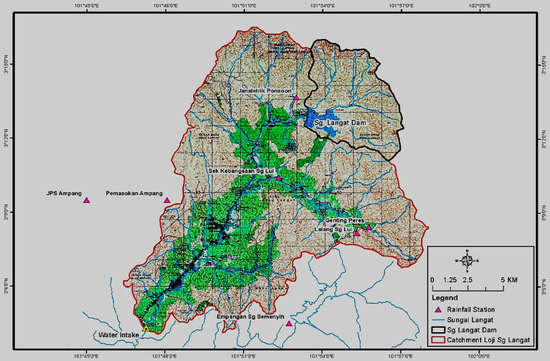
Figure 1.
Sg. Langat reservoir catchments area.
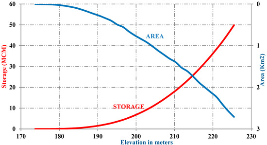
Figure 2.
Elevation versus storage volume and area for Sg. Langat reservoir.
The volumes of evaporation are a function of both the evaporation rate and the water surface area. Evaporation computations usually depend on the relationship between elevation and surface area. Table 1 shows a statistical analysis of historical data for the Sg. Langat reservoir over a period of 15 years from June 1996 to December 2010. In the table, it is apparent that the average minimum inflow occurs during the month of June, whereas the average maximum inflow occurs during September, with the average annual inflow being 46.78 × 10⁶ m3. The water intake demand must be determined to estimate the water demand for the Sg. Langat reservoir. We note that the water intake at the station is kept constant at 13.620 MCM per month.

Table 1.
Statistical analysis of historical inflows.
3. Materials and Methods
3.1. Artificial Neural Network (ANN)
ANNs (Artificial Neural Networks) are intensively interconnected processing units that use parallel computation algorithms. The inspiration for ANNs came from the desire to produce artificial systems capable of performing sophisticated (or perhaps intelligent) computations that mimic the routine performance of the human brain [13,14]. ANNs have been applied very successfully to solve complex problems in the environmental sciences [15] and water resources field [9]. One of the advantages of the ANN is its flexible mathematical structure that can identify nonlinear and complex relationships between input and output data, which has led to improvements in prediction accuracy, as compared with that of conventional models [16]. ANNs have various types of architecture, but the two most widely used are the feed-forward-back-propagation neural network (FBNN) and the radial basis function (RBF) network. In this work, we apply both the FBNN and RBF in the simulation of the reservoir relationship using hyperbolic tangent neurons in the hidden layers and a linear function at the output layer. We divided the data into two sets, with the first set used to train the models and the second set for testing and evaluating model performances. We describe the two networks proposed in this study in detail in the following paragraphs.
The feed-forward-back-propagation algorithm is the learning algorithm typically used in ANN applications, with the back-propagation system being the gradient descent technique used to minimize the network error. The FBNN is considered to be a multi-layer network that consists of input, hidden, and output layers. The input layer consists of some nodes I, hidden layers of J nodes, and an output layer of K nodes. Consequently, the output Rk can be written according to the formula published by Kothari [17]. This is shown below.
where:
- f = activation or transfer function,
- xi = input quantity,
- aij and bjk (i = 1,2, …, I; J = 1,2, …, J; k = 1,2, …, K) = weight values,
- aoj and bok = deviations.
f is a mapping rule for transferring neurons from input to output, and to indicate the nonlinear effect on the FBNN network [17]. There are FBNN transfer functions, but, for back-propagation, some principles are used, including monotonous non-decreasing, differentiable, and continuous functions. In this work, we use the sigmoid transfer function, which is defined as follows.
where the input values are in the range (0, 1). When a function is determined to be linear, for instance f(x) = x, all the ANN architecture will be linear in form from the input to the output layers [18]. In the FBNN structure (Figure 3), units in the same layer are not connected to each other, and connections among the layers are based on weight coefficients [19].
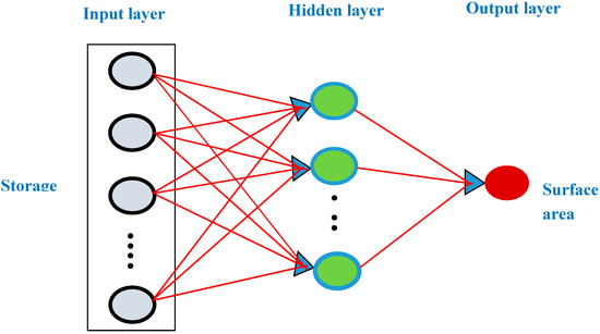
Figure 3.
Structure of the feed-forward-back-propagation neural network (FBNN).
Among the supervised and unsupervised training methods, the FBNN is considered to be a supervisory algorithm, where optimal factors are identified by regulating the weighted values in the network [20]. Optimal values are those for which the deviation between the target or actual value tk and the network output Rk reaches a minimum.
To generate an ANN output vector I = (i1, i2, …, ip) that is close to the target vector R = (r1, r2, …, rp), a learning process (also called training) is used to obtain the optimum bias vector V and weight matrices W, which reduces the error function that has been established in advance [20], as follows.
where:
- ti = desired output component I,
- ii = corresponding ANN output,
- p = number of nodes output,
- P = number of training patterns.
Training is a process in which the ANN connection weight is continuously adapted via continuous simulations. As with training, there are also supervised learning and unsupervised learning methods. The supervised learning process requires an exterior guide for the learning process and the size of the neural network affects the network generalization performance [21,22]. The authors of reference [23] provide a good review of the method used to determine a network structure to achieve satisfactory performance using training and generalization data.
For our analysis in this study, we use an RBF (Radial Basis Function), which is a common multi-layer with one hidden layer in the feed-forward network. We fed the input data to the input layer and the input layer transferred these data to the hidden layers, by adding the weighted input data obtained after the RBF was applied to every neuron via various dimensions. A Gaussian function is used to calculate the radial center in every hidden layer and then relay the distance from this center to the inputs. The spread and center are factors to be defined. The Gaussian function used in the hidden layers is very sensitive to data close to the center [24]. Lastly, the output layer receives values from the hidden layer and uses the newrbe function to obtain weighted values, which are presented as the output of the network.
In RBF networks [25], supervised learning is used, which involves a training data set. The RBF general formula is shown below.
where:
- Φ = activation function,
- c = center,
- R = metric,
- ((x − c)T·R−1·(x − c)) = distance between the center c and input x in the metric defined by R. In this situation, R = r2 for some scalar radius r, so the equation can be simplified to that shown in Equation (6).
The Euclidean length is indicated by rj, which measures the distance in the radial between the weight and radial center Y(j) = (w1j, w2j, …, wmj), where wij and yi = output and datum vector y = (y1, y2, …, ym) [26], which can be expressed as follows.
The appropriate transfer function is applied to rj as follows.
Lastly, the output layer (k = 1) obtains the weighted linear combination of Φ = (rj), as follows.
Supervised learning requires signals to guide the learning or target pattern, with the aim to discover the optimum weight by determining the minimum error between the actual and target outputs. In the learning of the RBF, the weight factors are modified to obtain target outputs that match the given inputs. A variety of training algorithms have been proposed for RBFNN (Radial Basis Function Neural Network) learning [27].
3.2. Optimization Model
SDP is a useful approach for problem decision-making that utilizes a decisions sequence that responds to outcomes and progresses over time [28]. Using SDP, time units in the reservoir process system are considered to be stages in the framework optimization, with the water storage defined at each stage as the system state, and the inflow is a stochastic feature that can be efficiently addressed. The randomness of the reservoir operation in SDP can be expressed by probabilities, with various probabilities representing different inflow levels that can be combined for framework optimization in every stage [29]. The SPD recursive function mode used in this study is as follows.
where:
- = objective function,
- St = storage at the beginning time of period t,
- Rt = release during the time period t,
- C (.) = function of immediate return,
- Qt = inflow during month t,
- α = SDP algorithm discount rate.
In this work, we established a monthly SDP stepped model with a fitness function and an objective function to reduce the monthly squared deviation release deficit.
The objective function is as follows.
where:
- t = month index,
- N = operating horizon in months,
- R(t) = release in month t,
- D(t) = demand in month t.
Equation (11) above incorporates storage, mass balance, surplus constraints, and evaporation, with inflow and storage discretized into 100 classes and 60 classes, respectively, as shown in Figure 4. The basic elements for developing a dynamic program is to identify the state variables. The state variables are variables describing the state of a system at any stage n. A state variable can be discrete or continuous. The state variables of the system in a dynamic programming model have the function of linking succeeding stages so that, when each stage is optimized separately, the resulting decision is automatically feasible for the entire problem. Furthermore, it allows one to make optimal decisions for the remaining stages without having to re-compute the effects of future decisions on the objective function. For a reservoir operation, storage can be the state variable(s). In this context, the state in the SDP formulation is to discretize the storage, which is referred to as representative values. The storage variable is restricted to finite sets of discrete storage. The sets of discrete storages are chosen so that the entire possible ranges for these variables are considered. The discrete representation of the storage volume is based on the study that the effective storage has to be divided into n intervals. The medium value of each interval is the representative storage value, and, hence, n+2 representative storage levels can be obtained, including the dead storage and the full storage. The storage state would be represented by the representative storage that is the nearest to this storage state. In Figure 4, the first class of the inflow state variable has zero value, whereas the last inflow has no upper bound, so it has the highest historical corresponding inflow value.
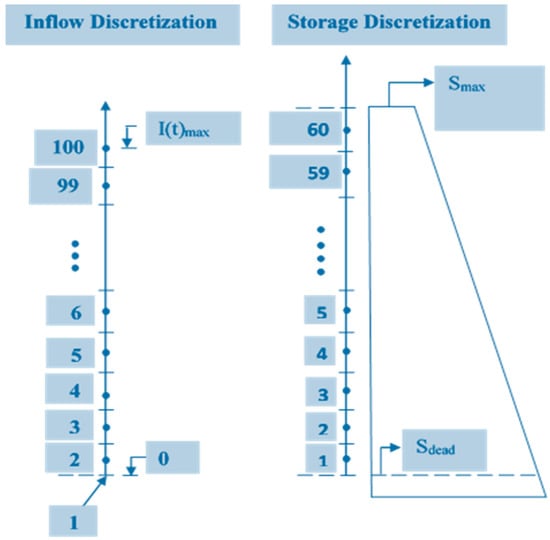
Figure 4.
Discretization used by the SDP model for every month t = 1, …, 12. The dots along the vertical axes represent discrete values. The numbers indicate classes.
Figure 5 shows the proposed SDP-ANN model flow chart. In the model application process, first, the stream inflows are discretized and the functioning storage volumes (level) are determined. Then, to obtain the solution, the SDP method creates objective function values up to the last stage of zero for every state variable combination. ANN is used to simulate the reservoir system. Later, the procedure continues backward along the temporal phases. Every iteration contains a T phase that finishes one annual cycle. Then, the algorithm discovers the end period storage levels for every discretized class, starting with the average inflow and storage levels of the current period. Convergence occurs after these iterations because the Markov characteristics lead to transitions in the possibility matrix combined with the recursive equation.
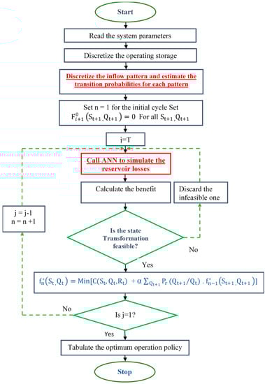
Figure 5.
Flow chart for the proposed SDP-ANN model solution.
3.3. Model Evaluation Criteria
RBF networks, an FBNN network, and regression models were used to simulate the relationship between the surface area and the storage volume of Sg. Langat reservoir. There is no conclusive test available for evaluating model performance. Therefore, various indicators were used. Basically, we evaluated the models’ performance based on the actual and simulated data, using the relative root mean square error (RRMSE), root mean square error (RMSE), and mean absolute percentage error (MAPE). The formulas used for these indicators are as follows.
It is recommended that RMSE, RRMSE, and MAPE be used as evaluation indices for prediction models [19]. The RMSE provides an aggregate measure of the magnitude of the errors, which is determined by the differences between the actual and predicted data, based the model output, as a single value. Therefore, RMSE is considered to be a vital and fair measure of the accuracy of a model when comparing the results obtained from several models. Similarly, the RRMSE provides the same measure. However, it is a more suitable measure of scale-dependent datasets, which is the case in the current study regarding the elevation-surface-area-storage relationship. Lastly, the MAPE is essential for evaluating model performance since it represents the model accuracy as a percentage, which makes it easy to compare the performances of different models.
Generally, evaluations of models using the RRMSE and RMSE are based on a comparison of the estimated errors between the actual and simulated results. The model with the smallest error is considered the best. A model simulation with an MAPE of around 30% is considered to be acceptable [30], and that, with an MAPE value of 5% to 10%, is considered to be very accurate. Lastly, we measured the efficiency of the proposed model using the coefficient of efficiency (CE), as shown in Equation (15). The maximum possible CE value is 1, which indicates that the model performance is effective.
where:
- = predicted value,
- = actual value,
- = predicted mean value,
- = actual mean value,
- = number of forecasting periods.
3.4. Evaluation Indicators for the Optimization Model
3.4.1. Reliability (R)
Reliability is the oldest and the most utilized parameter in water resource systems. The equation was proposed by the authors of reference [31], as follows.
where S is the variability of the system state under consideration. The definition most often applied and most widely accepted is the reliability of occurrence, which is expressed as follows:
where d(j) is the duration of the failure event, M is the number of failure events, and T is the total number of time intervals.
3.4.2. Resilience (R)
Resilience is the speed with which a system returns to a satisfactory state after having been in an inacceptable state. The authors in reference [31] expressed resilience as a conditional probability, as follows:
where S(t) is the variability of the system state under consideration. Resilience is described as being equal to the mean time inverse of the time system during the unsatisfactory state.
where d(j) is the duration of the failure event and M is the total number of failure events. The authors of reference [32] defined resilience as the maximum duration of time a system spends in an inacceptable state.
To make the definition used in reference [32] comparable with that of Res1 in Equation (19), resilience can be expressed by the inverse of the maximum duration.
3.4.3. Vulnerability (V)
Vulnerability, as introduced by the authors of reference [31], is the likely damage incurred by a failure event, which is expressed as follows.
where h(j) is the jth occurrence of a severe outcome with an inacceptable state and e(j) is the h(j) probability, which is the occurrence of a severe outcome with an inacceptable state. The authors of references [31,33] developed a measurement of vulnerability based on the total water deficit during the entire occurrence as F, i.e., the volume of the deficit. This description is suitable for reservoirs, since the severe outcome state in reservoirs often results in them being empty (h(j) = 0). To simplify Equation (21), the authors of these studies considered the probability of each event to be equal, i.e., e(1) = … = 1/M = e(M), where M is the number of failure events. Consequently, the approximate vulnerability is expressed as the mean deficit value event v(j), as follows.
4. Results and Discussion
In this work, we utilized the ANN technique to simulate the reservoir system. We selected this approach based on the experience of previous studies that had used regression models to simulate the storage and surface area values of reservoirs. However, we also took into consideration the shortfalls of the ANN in comparison to regression models regarding the storage–surface area relationship. The first stage in the ANN is training, since this stage reduces the error by finding the best connection set and threshold value that enables the ANN model to generate a result that is close or equal to the targets. We adjusted the expected mean square error (MSE) obtained in the training phase to 10−4, based on the principle that considers the best model performance will have the lowest MSE value during the training phase.
4.1. Storage–Surface-Area Relationship
The performances of the simulation methods were compared using various indicators including the MAPE, RRMES, RMSE, and CE. Figure 6 and Figure 7 show the test results as percentage errors for the reservoir simulations of the elevation-surface-storage relationship. The authors of Reference [34] reported that percentage error values provide a basis for determining model accuracy. In the figure, we can see that the percentage error of the predicted surface area continually decreases with respect to elevation (the height from the bottom of the reservoir) up to 199.63 m. In addition, we can see a sudden fluctuation in the percentage error pattern in the predicted surface area when the altitude is between 184.4 m and 196.59 m. This is due to the fact that, upstream of the reservoir, a dam had formed naturally without any human interference to re-shape it and sediment had accumulated over the years of operation since completion of the dam. As such, the vertical, horizontal, and longitudinal cross-sections of the reservoir are completely irregular. As a result, there can be sudden, abrupt, or rapid changes in the horizontal cross-section at this range of elevation due to the unexpected changes in the surface area, which may cause fluctuation in the accuracy of the predicted surface area. Furthermore, the same observation is noted in the FBNN and RBF results, which confirms that the relationship between the elevation and surface area within this particular elevation range is highly nonlinear, as illustrated in Figure 7.
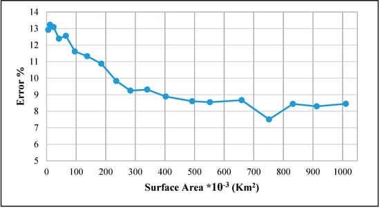
Figure 6.
The AR storage-surface area relationship percentage error.
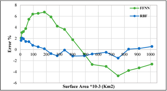
Figure 7.
Percentage errors of RBF and FBNN regarding the storage-surface area relationship.
Table 2 lists the FBNN, RBF network, and regression model analyses with regard to the surface area and its relationship to water storage at Sg. Langat reservoir. In addition, the table lists the CE values of the models. The results reveal that the RBF model has a higher accuracy and productivity during the testing phase, with a CE value of 0.9993. This result confirms that the RBF has higher reliability and accuracy for simulating the surface area and storage relationship. To be considered a very accurate model, the MAPE values for the Sg. Langat reservoir model simulation should be less than 1%. The result presented in Table 2 indicates that the RBF has a MAPE value of 0.982%, and can, thus, be considered to be very accurate. However, the AR and FBNN models have MAPE values of 10.2% and 3.879%, respectively, which reveal that the RBF model performed better than the AR and FBNN models. Moreover, when the RRMSE and RMSE values are close to zero, there is a smaller degree of error in the simulation phase. In the table, the RBF model has an RRMSE value of 0.011 and an RMSE of 0.009 km2, which are nearly zero and are about half those of the AR and FBNN models. This further confirms that the RBF system yields greater simulation accuracy. From these simulation results and the rigorous confirmation procedures applied, it is clear that the RBF application performs better with regard to the relationship between surface area and storage of Sg. Langat reservoir than the AR and FBNN models. In summary, the AR and FBNN models generated greater errors than the RBF model, which obtained higher CE values and lower RRMSE and RMSE values.
Table 2.
Performance indicators of the AR, FBNN, and RBF models regarding the storage-surface-area relationship.
Regarding the errors associated with different models that use different methods for simulating the surface area, as shown in Figure 6; Figure 7, the RBF method has an error with a respective minimum and maximum of −2 and 2. The error of the FBNN is higher, with a minimum error of −5 and a maximum error of less than 7, as shown in Figure 7. The AR method error exceeded those of the other two methods, and its error value range differs in nature. Its results are presented in Figure 6. Moreover, we identified a linear relationship between the surface area and storage in the AR model results, which indicates that the model has a higher error than the ANN models, whose error values are close to the axis. When the models were evaluated, the RBF showed the best performance. From the tables and figures obtained from the testing set, the RBF model also yielded better results in terms of accuracy, as compared to the AR and FBNN models, with constant values of RRMSE and RMSE. We also proved that the AR method is able to handle the nonlinear relationship of the reservoir. It is, thus, certain that flexible models can yield the lowest MAPE, RRMSE, and RMSE errors, with the AR results revealing that the AR model has the necessary flexibility for modeling the relationship between the storage and surface area.
The ANN modeling method is convenient for modeling hydrological processes. The ANN is a powerful and useful tool that has been utilized for mapping complicated relationships and achieving better performance than conventional methods. The results obtained from the simulation analysis proved that the reliability and accuracy of the ANN is greater than those of the other methods, and the storage-surface-area relationship was accurately determined by the ANN modeling method in this study. The ANN outputs confirmed the superiority of ANN over traditional simulation methods used for solving hydrological problems. The ANN model developed in this study provides an accurate and beneficial means for resolving problems related to water storage.
4.2. ANN or AR with Stochastic Dynamic Programming as a Simulation Model
SDP models with either an ANN or AR were established to develop effective policies for the reservoir operation. Figure 8 shows the SDP-ANN and SDP-AR cumulative penalty models in which the reservoir system used a penalty function to measure performance and determine the decision-making method that would contribute the most to the reservoir operation [35]. A decision-making process was developed to improve the water release schedule to meet operational requirements and target demands with reference to the target demand. To keep forces to a minimum, a penalty function was implemented. The use of the choice system was, thus, expected to improve the resiliency and reliability with minimum cumulative and vulnerability penalty values. The existing model (Model 2) integrated the SDP and ANN, and Figure 8 shows that the obtained cumulative penalty value for Model 1 is 0.39 whereas that for Model 2 is 0.36. The obtained minimum penalty value from the Model 2 SDP-ANN are identical to those of the other models, which reveals that Model 2 performs better by 8.3% than Model 1.
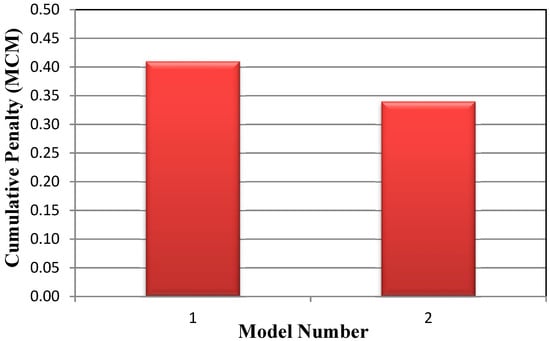
Figure 8.
Cumulative penalty values of SDP-AR (Model 1) and SDP-ANN (Model 2) models.
The performance indicators used for water demand of the reservoir downstream section for the 15-year period were limited to resiliency, vulnerability, and reliability. We found the reliability of Model 1 to be 0.66% and of Model 2 to be 0.71%. The water supply reliability is improved by 7.5% by using Model 2. Over the 175 months of the study period, we determined water supply shortages had occurred, and that Model 2 found 51 months to have had unsatisfactory water supply, whereas Model 1 found that 60 months had experienced shortages in water supply. In addition, Figure 9 shows the reliability, resilience, and vulnerability results. The resilience value obtained for Model 2 is 6.3% better than that of Model 1, which indicates that Model 2 is more suitable than Model 1. The vulnerability values, which are based on the non-supply of expected water, was 0.38 for Model 1 and 0.36 for Model 2, which indicates that the Model 2 value was 5.5% better than Model 1.
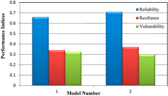
Figure 9.
Performance indices regarding the supply of water demand for SDP-AR (Model 1) and SDP-ANN (Model 2) models.
Reservoirs are essential facilities that can provide sustainable and reliable sources of water for all water users downstream. For the current case study, it is vital to ensure that the proposed operation rules can provide sustainable functionality for present and future water demands. Several approaches are available for considering the sustainability of dams and reservoir operations. For example, a sustainable evaluation could involve the river ecology, flood and drought control, sediment management, river water quality, and water resources allocation. The main concern of decision-makers in the case study was to ensure the sustainable allocation of water resources for downstream water users. To guarantee that the rules generated for optimal reservoir operation would provide sustainable usage of the available water resources, several evaluation metrics must be considered. In this study, we focused on three performance indices, including reliability, resilience, and vulnerability to determine the performance of the generated operation rules based on a new proposed reservoir simulation model utilizing the RBF model.
5. Conclusions
In this study, we established and applied an SDP-ANN model, and compared its results with those of the SDP-AR model. The accurate simulation of a reservoir is considered to be a vital step in achieving appropriate operational policies regarding water release from the reservoir. In practical terms, the main application of the proposed optimization model is to generate sustainable and reliable operational policies for managing the available water resources to meet and match the temporal water usages downstream from the reservoir. We developed SDP-ANN and SDP-AR models using the same objective function and inflow data. The natural nonlinearity of the physical processes is the main challenge when developing a reservoir system simulation, especially when using linear systems such as the AR method. Therefore, we used a nonlinear computational technique to simulate the system. A comparison of the performances of the AR and ANN models highlights the superiority of the ANN. Moreover, the results reveal that the proposed Model 2 is less vulnerable and more resilient and reliable than Model 1. In summary, the SDP-ANN model performs better than the SDP-AR model for the purposes of developing operational policies for the reservoir system.
Although the proposed model effectively improved the operation rules for the reservoir operation and enabled the generation of a sustainable and reliable water release policy, there are two major disadvantages in this model structure. First, the proposed optimization model (SDP) experienced a slow convergence process, and might become trapped in local minima while searching for the global optimal objective function. Therefore, we recommend that the potential for utilizing a more advanced optimization algorithm be investigated as an alternative, such as the meta-heuristic optimization algorithm. The meta-heuristic optimization algorithm may realize faster convergence than SDP and more efficiently obtain the global optima, which means it is more effective when applied to real-time operation of the dam and reservoir water system. Second, the proposed model has only been examined with respect to water resources allocation. In future research, more sustainable factors should be considered as evaluation metrics, such as sediment management, water quality, and the river ecosystem, to determine the sustainable functionality of the operational policies from multi-objective angles.
Author Contributions
Conceptualization, S.S.F. (Sabah Saadi Fayaed), L.S.H., and A.E.-S. Data curation, S.S.F. (Sabah Saadi Fayaed), S.S.F. (Seef Saadi Fiyadh), W.J.K., and S.K. Formal analysis, S.S.F. (Sabah Saadi Fayaed), S.S.F. (Seef Saadi Fiyadh), S.K., N.S.M., and W.Z.B.J. Funding acquisition, A.N.A., L.S.H., and A.E.-S. Investigation, W.J.K., A.N.A., and C.M.F. Methodology, S.S.F. (Sabah Saadi Fayaed), S.S.F. (Seef Saadi Fiyadh), H.A.A., and A.E.-S. Project administration, L.S.H. Resources, W.J.K. and C.M.F. Software, H.A.A. and W.Z.B.J. Validation, A.N.A. and N.S.M. Visualization, A.N.A., R.K.I., and C.M.F. Writing–original draft, S.S.F. (Sabah Saadi Fayaed), S.S.F. (Seef Saadi Fiyadh), and A.E.-S. Writing–review & editing, H.A.A., R.K.I., N.S.M., and W.Z.B.J.
Funding
This research financially supported from Bold 2025 grant coded RJO:10436494 by the Innovation & Research Management Center (iRMC), Universiti Tenaga Nasional (UNITEN), Malaysia, and research grant coded UMRG RP025A-18SUS funded by the University of Malaya and by Ministry of Higher Education Malaysia from Fundamental Research Grant Scheme (FRGS, Grant No: FRGS/1/2019/TK01/UNITEN/02/3).
Acknowledgments
The authors appreciate so much the facilities support by the Civil Engineering Department, Faculty of Engineering, University of Malaya, Malaysia.
Conflicts of Interest
The authors declare no conflict of interest.
References
- Jothiprakash, V.; Shanthi, G. Single reservoir operating policies using genetic algorithm. Water Resour. Manag. 2006, 20, 917–929. [Google Scholar] [CrossRef]
- Kalaji, H.M.; Sytar, O.; Brestic, M.; Samborska, I.A.; Cetner, M.D.; Carpentier, C. Risk Assessment of Urban Lake Water Quality Based on in-situ Cyanobacterial and Total Chlorophyll-a Monitoring. Pol. J. Environ. Stud. 2016, 25, 655–661. [Google Scholar] [CrossRef]
- Simonovic, S.P. Reservoir systems analysis: Closing gap between theory and practice. J. Water Resour. Plan. Manag. 1992, 118, 262–280. [Google Scholar] [CrossRef]
- Yeh, W.W.G. Reservoir management and operations models: A state-of-the-art review. Water Resour. Res. 1985, 21, 1797–1818. [Google Scholar] [CrossRef]
- Labadie, J.W. Optimal operation of multireservoir systems: State-of-the-art review. J. Water Resour. Plan. Manag. 2004, 130, 93–111. [Google Scholar] [CrossRef]
- Wurbs, R.A. Reservoir-system simulation and optimization models. J. Water Resour. Plan. Manag. 1993, 119, 455–472. [Google Scholar] [CrossRef]
- Zarghami, M.; Szidarovszky, F. Stochastic-fuzzy multi criteria decision making for robust water resources management. Stoch. Environ. Res. Risk Assess. 2009, 23, 329–339. [Google Scholar] [CrossRef]
- Maqsood, I.; Huang, G.; Huang, Y.; Chen, B. ITOM: An interval-parameter two-stage optimization model for stochastic planning of water resources systems. Stoch. Environ. Res. Risk Assess. 2005, 19, 125–133. [Google Scholar] [CrossRef]
- Lv, Y.; Huang, G.; Li, Y.; Yang, Z.; Liu, Y.; Cheng, G. Planning regional water resources system using an interval fuzzy bi-level programming method. J. Environ. Inform. 2010, 16, 43–56. [Google Scholar] [CrossRef]
- Li, Y.; Huang, G.; Nie, S. An interval-parameter multi-stage stochastic programming model for water resources management under uncertainty. Adv. Water Resour. 2006, 29, 776–789. [Google Scholar] [CrossRef]
- Mahdouh, S.; Van Oorschot, H.; De Lange, S. Statistical Analysis in Water Resources Engineering; AA Balkema: London, UK, 1993. [Google Scholar]
- Najah, A.A.; El-Shafie, A.; Karim, O.A.; Jaafar, O. Water quality prediction model utilizing integrated wavelet-ANFIS model with cross-validation. Neural Comput. Appl. 2012, 21, 833–841. [Google Scholar] [CrossRef]
- McCulloch, S.W.; Pitts, W. A logical calculus of the ideas immanent in nervous activity. Bull. Math. Biophys. 1943, 5, 115–133. [Google Scholar] [CrossRef]
- Rumelhart, D.E.; Hinton, G.E.; Williams, R.J. Learning representations by back-propagating errors. Nature 1986, 323, 533–536. [Google Scholar] [CrossRef]
- Flood, I.; Kartam, N. Neural networks in civil engineering. I: Principles and understanding. J. Comput. Civ. Eng. 1994, 8, 131–148. [Google Scholar] [CrossRef]
- Sarle, W.S. Neural Networks and Statistical Models. In Proceedings of the Nineteenth Annual SAS Users Group International Conference, Dallas, TX, USA, 10–13 April 1994. [Google Scholar]
- Kothari, R.; Agyepong, K. On lateral connections in feed-forward neural networks. In Proceedings of the Neural Networks, Washington, DC, USA, 3–6 June 1996; pp. 13–18. [Google Scholar]
- Barron, A.R. Universal approximation bounds for superpositions of a sigmoidal function. IEEE Trans. Inf. Theory 1993, 39, 930–945. [Google Scholar] [CrossRef]
- El-Shafie, A.; Taha, M.R.; Noureldin, A. A neuro-fuzzy model for inflow forecasting of the Nile river at Aswan high dam. Water Resour. Manag. 2007, 21, 533–556. [Google Scholar] [CrossRef]
- El-Shafie, A.; El-Manadely, M. An integrated neural network stochastic dynamic programming model for optimizing the operation policy of Aswan High Dam. Hydrol. Res. 2011, 42, 50–67. [Google Scholar] [CrossRef]
- Baum, E.B.; Haussler, D. What Size Net Gives Valid Generalization? Neural Comput. 1989, 1, 151–160. [Google Scholar] [CrossRef]
- Agyepong, K.; Kothari, R. Controlling hidden layer capacity through lateral connections. Neural Comput. 1997, 9, 1381–1402. [Google Scholar] [CrossRef]
- Bishop, C.; Bishop, C.M. Neural Networks for Pattern Recognition; Oxford University Press: New York, NY, USA, 1995. [Google Scholar]
- El-Shafie, A. Neural network nonlinear modeling for hydrogen production using anaerobic fermentation. Neural Comput. Appl. 2014, 24, 539–547. [Google Scholar] [CrossRef]
- Walczak, B.; Massart, D. The radial basis functions—partial least squares approach as a flexible non-linear regression technique. Anal. Chim. Acta 1996, 331, 177–185. [Google Scholar] [CrossRef]
- Fausett, L. Fundamentals of Neural Networks; Prentic Hall Intenational, Inc.: Upper Saddle River, NJ, USA, 1994. [Google Scholar]
- Piotrowski, A.P.; Osuch, M.; Napiorkowski, M.J.; Rowinski, P.M.; Napiorkowski, J.J. Comparing large number of metaheuristics for artificial neural networks training to predict water temperature in a natural river. Comput. Geosci. 2014, 64, 136–151. [Google Scholar] [CrossRef]
- Michalland, B.; Parent, E.; Duckstein, L. Bi-objective dynamic programming for trading off hydropower and irrigation. Appl. Math. Comput. 1997, 88, 53–76. [Google Scholar] [CrossRef]
- Isles, P.D.; Giles, C.D.; Gearhart, T.A.; Xu, Y.; Druschel, G.K.; Schroth, A.W. Dynamic internal drivers of a historically severe cyanobacteria bloom in Lake Champlain revealed through comprehensive monitoring. J. Great Lakes Res. 2015, 41, 818–829. [Google Scholar] [CrossRef]
- Joyner, W.B.; Boore, D.M. Measurement, characterization, and prediction of strong ground motion. in Earthquake Engineering and Soil Dynamics II. In Proceedings of the American Society of Civil Engineers Geotechnical Engineering Division Specialty Conference, Park City, UT, USA, 27 June 1988. [Google Scholar]
- Hashimoto, T.; Stedinger, J.R.; Loucks, D.P. Reliability, resiliency, and vulnerability criteria for water resource system performance evaluation. Water Resour. Res. 1982, 18, 14–20. [Google Scholar] [CrossRef]
- Moy, W.S.; Cohon, J.L.; ReVelle, C.S. A programming model for analysis of the reliability, resilience, and vulnerability of a water supply reservoir. Water Resour. Res. 1986, 22, 489–498. [Google Scholar] [CrossRef]
- Jinno, K. Risk assessment of a water supply system during drought. Int. J. Water Resour. Dev. 1995, 11, 185–204. [Google Scholar] [CrossRef]
- Johnson, A.C., Jr.; Johnson, M.B.; Buse, R.C. Econometrics: Basic and Applied; Prentice Hall & IBD: New York, NY, USA, 1987. [Google Scholar]
- Karamouz, M.; Houck, M.H. Comparison of stochastic and deterministic dynamic programming for reservoir operating rule generation 1. JAWRA J. Am. Water Resour. Assoc. 1987, 23, 1–9. [Google Scholar] [CrossRef]


© 2019 by the authors. Licensee MDPI, Basel, Switzerland. This article is an open access article distributed under the terms and conditions of the Creative Commons Attribution (CC BY) license (http://creativecommons.org/licenses/by/4.0/).