Agricultural Water Management Model Based on Grey Water Footprints under Uncertainty and its Application

Abstract

The grey water footprint theory was introduced into a fractional programming model to alleviate non-point source pollution and increase water-use efficiency through the adjustment of crop planting structure. The interval programming method was also incorporated within the developed framework to handle parametric uncertainties. The objective function of the model was the ratio of economic benefits to grey water footprints from crop production, and the constraints contained water availability constraints, food security constraints, planting area constraints, grey water footprint constraints and non-negative constraints. The model was applied to the Hetao Irrigation District of China. It was found that, based on the data in the year of 2016, the optimal planting plans generated from the developed model would reduce 34,400 m³ of grey water footprints for every 100 million Yuan gained from crops. Under the optimal planting structure, the total grey water footprints would be reduced by 21.9 million m³, the total economic benefits from crops would be increased by 1.138 billion Yuan, and the irrigation water would be saved by 44 million m³. The optimal results could provide decision-makers with agricultural water use plans with reduced negative impacts on the environment and enhanced economic benefits from crops.

1. Introduction

As populations expand, economies grow and dietary preferences change, the demand for agricultural production is expected to rise in the future [1,2]. For the countries that lack water and land resources, the use of agrochemicals, such as chemical fertilizers and pesticides, has been intensified to squeeze more food out of the land [3,4]. However, the leaching of agrochemicals may cause the pollution of surface and ground water [5,6]. Minimizing the pollution caused by cultivation activities while ensuring food production has become a pressing issue. Optimizing the planting structure (planting areas of different crops) could be an effective way to reduce the negative impacts of crop production on the environment and promote an efficient and sustainable use of water resources in agriculture.

Previously, programming models have been widely used to address optimization problems in many fields [7,8,9,10,11]. There also were many attempts in agricultural systems which used optimization methods [12,13]. Earlier attempts were largely focused on single-objective optimization of agricultural systems, where economic performance was considered as the primary objective to maximize financial return of farmers [14]. In these models, the complexity of ecological effects was largely ignored. Recently, more targets were considered in the optimization of agricultural systems, and a number of studies based on multi-objective programming approaches were reported [15,16]. Multi-objective methods usually combined objectives of multiple aspects into a single measure on the basis of subjective assumptions, where identification of weighting factors or economic indicators was considered difficult. Selecting solutions from the Pareto front would bring additional difficulties to optimization decisions. Moreover, multi-objective programming methods could not measure system efficiency represented as output/ input ratios [17]. Fractional programming is an effective tool to deal with optimization of ratios, where the objective is the quotient of two functions (e.g., cost/time, cost/volume, or output/input) [18]. It could directly compare objectives of different aspects through the original magnitudes and provide an unbiased measurement of system efficiency [17]. There were many studies which used fraction programming in agricultural systems [19,20].

However, the previous fractional programming models couldn’t handle both uncertainties and negative eco-environmental impacts of crop production simultaneously. Economy parameters in the model (such as crop prices, planting costs, and sewage treatment costs) fluctuate with the market. Technology parameters (such as crop productivity and irrigation water utilization coefficient) vary with natural environmental factors (e.g., soil and climate). Hydrology parameters are not fixed in real-world problems as well. For example, pollution leaching rate varies with irrigation water volume and geographical areas. Moreover, the application and utilization rates of agrochemicals to different farmlands vary with specific crops. Therefore, pollution leaching has large spatial uncertainties. In addition, there exist uncertainties in different periods. The matter flow mediated downward movement of pollutants varies with the irrigation periods. During different irrigation periods, the factors, such as the temperature, the stage of crop growth and the amount of irrigation, vary, while the matter flow mediated downward movement of pollutants is related to these factors. Inexact optimization methods could take into account various complexities. In order to quantitatively describe the complexities in ecological effects from the crop production process described above, it is necessary to introduce the concept of grey water footprint.

The grey water footprint [21] allows quantifying the negative impacts of agricultural production on the water quality. The grey water footprint refers to the volume of water required to dilute the contaminants that accompany the production process [22]. Previous studies [23,24] only evaluated and calculated the grey water footprint, but could not support related decisions. For example, Cao et al. [25] applied the grey water footprint theory to the Hetao Irrigation District, calculated the grey water footprint of grain production, but couldn’t propose a concrete plan for planting structure adjustment. A number of studies have optimized crop planting structures based on water footprint theory [26,27,28]. Nevertheless, previous studies could barely handle uncertainties in the grey water footprints or incorporate grey water footprints into decision processes.

Therefore, an agricultural water management model based on grey water footprints, fractional programming and interval programming is established in this study. Considering the complexity of pollution leaching during crop production, the study quantifies the negative effects of crop production using the grey water footprint theory. The model based on interval fractional programming aims at maximizing the economic benefits from unit grey water footprint and seeks a comprehensive and optimal planting plan. It also takes various uncertainties in factors, such as economy, technology, and hydrology, into account. The model could provide a theoretical basis and serve as a decision-support tool for the optimization of crop planting structure.

2. Complexities of Agricultural Water Management Problems

The parameters in agricultural systems and their interrelationships are uncertain which can be reflected in many aspects of hydrology, economy and technology. Uncertainty increases the complexity of the optimization process. Ignoring these uncertainties may lead to large errors and even erroneous decisions [29]. Therefore, it is important to consider these uncertainties into the process of building the model, which can make the model closely reflect real-world problems.

Agrochemical transfer process is illustrated in Figure 1. Agrochemicals applied in farmland soil are partially absorbed or utilized during crop growth, some of which remain in the soil. In addition, some agrochemicals are inevitably lost due to leakage, volatilization, denitrification and runoff [30]. The loss of agrochemicals will leach deep into the soil, enter the groundwater with irrigation or rainfall, or be discharged into the water body through farmland runoff. For arid or semi-arid areas with features of drought, pollutants are mainly lost through leaching. The leaching of pollutants in the soil requires two conditions, namely the accumulation of contaminant [31] and the matter flow mediated downward movement of pollutants [32]. Due to the small rainfall in arid or semi-arid areas, the irrigation processes become the main driving factor for contaminant leaching to the deep layer of the soil and entering the groundwater. The leaching of agrochemicals not only causes the pollution of surrounding environment, but also exacerbates the eutrophication of water bodies.

Pollutant discharges in different types of farmlands, different geographical regions and different periods vary. Considering the large area of the agricultural system, the dilution of pollutants in different planting areas is actually completed by different water bodies. The contaminants caused by agricultural production in a certain area may discharge to near and distant waterbody because of the fluidity of water and human impact [33]. The composition of non-point source pollutants is complex, and the same water can dilute component 1, component 2, and component 3, which is shown in Figure 1. Grey water footprint is determined by the pollutant that requires the most dilution [34]. There is a great deal of uncertainties in the grey water footprints from crop production.

Taking nitrate, which is the most common and widespread contaminant in groundwater, as an example. Having a thorough understanding of the interactive processes within the nitrogen migration is important for decision making [35]. A previous study has shown that nitrogen loss through leaching is mainly nitrate nitrogen [30]. Due to the different application and utilization rates of nitrogen fertilizer, the mediated downward movement of nitrogen in different types of farmland soils varies [36]. Hu et al. found that the leached nitrogen content was positively correlated with the amount of irrigation water in the dry land [37]. Therefore, there are spatial differences in leaching processes, which need to be considered separately for different crops and different geographical regions. In addition, there are still temporal uncertainties in the leaching of nitrogen. Experimental results of Ou et al. indicated that the nitrogen leaching in the field during the autumn irrigation period played a decisive role [38]. During summer irrigation, as the temperature is high, the microbial activity is strong and the denitrification reaction is easy to occur, nitrate nitrogen is first converted into NO₂ and N₂ and then released to the atmosphere. Moreover, summer irrigation happens in the growth stage of crops when transpiration is strong, it has an impeding effect on the matter flow mediated downward movement of nitrogen. The matter flow mediated downward movement of nitrogen during summer irrigation is not obvious, which mainly occurs in the surface of soil rather than the groundwater. It could be seen that the leaching of nitrogen has both spatial and temporal variations.

3. Methodology

3.1. Interval Grey Water Footprints Estimation Method

Uncertainties existing in the processes of pollutant migration and transformation could result in uncertainties in grey water footprints. The uncertainties could be handled by interval programming [39,40], fuzzy programming [20,41,42] and stochastic programming [43,44] methods, according to the formats in which uncertainties are expressed. Solving exact models is relatively easy because the parameters are deterministic. For inexact models, the values of parameters are uncertain. Usually, distribution information or membership functions of parameters are difficult to obtain; on the contrary, the lower and upper bounds of uncertain parameters can be easily obtained [45]. Interval mathematical method is capable of handling input uncertainty expressed as interval parameters. An interval parameter $a^{\pm }$ does not require distributional information, and can be expressed as $a^{\pm }=[a^{-},a^{+}]$, where $a^{-}$ and $a^{+}$ represent the lower and upper bound, respectively [46]. Therefore, an interval grey water footprints estimation method is developed in this study, which is based on the grey water footprint method proposed by Hoekstra et al [22,33].

The total grey water footprint $G^{\pm }$ is summed by the grey water footprint related to each water body:

$$G^{\pm }={\displaystyle \sum W{g}_j^{\pm },j=1,2,\cdots ,n}$$

(1)

where $W{g}_j^{\pm }$ is grey water footprint of the j-th water body.

$$W{g}_j^{\pm }=\frac{P{l}_j^{\pm }}{C_{j-\max }^{\pm }-C_{j-net}^{\pm }},j=1,2,\cdots ,n$$

(2)

$$P{l}_j^{\pm }={\lambda }_j^{\pm }·{\mu }^{\pm }·TP{l}^{\pm }\omega$$

(3)

where $P{l}_j^{\pm }$ is the discharge of pollutant into the j-th water body; $C_{j-\max }^{\pm }$ is the maximum concentration of pollutant in the j-th water body allowed by the water quality standard; $C_{j-net}^{\pm }$ is the initial concentration of pollutant in the j-th water; $TP{l}^{\pm }$ is the total discharge of pollutant; ${\lambda }_j^{\pm }$ is the proportional coefficient of the pollutant discharged into the j-th water body; and ${\mu }_i^{\pm }$ is the leaching rate of the pollutant.

3.2. Agricultural Water Management Model Based on Grey Water Footprints

This paper establishes an agricultural water management model based on grey water footprints to deal with the optimization of ratio and uncertainties in pollutant migration and transformation. The model is based on the grey water footprint theory, taking into account both the economic benefits and the grey water footprints resulting from the loss of agrochemicals associated with the crop growth period and the end of the growing season. The optimized results could maximize the economic benefits from a unit grey water footprint during crop production and reasonably determine the areas of crops in different regions.

The model consists of five equations: objective function equation, water availability constraints, food security constraints, planting area constraints, grey water footprint constraints, and non-negative constraints. The following is a detailed description of the model formulation.

3.2.1. Objective Function

$$\begin{array}{l}\max f=\max f_1/f_2=\max [{\displaystyle \sum _{i=1}^I{\displaystyle \sum _{j=1}^J(Y_{ij}^{\pm }·P_j^{\pm }-C_j^{\pm })·S_{ij}^{\pm }-{\displaystyle \sum _{i=1}^I{\displaystyle \sum _{j=1}^J(Q_{aij}^{\pm }+Q_{bij}^{\pm })·S_{ij}^{\pm }·E^{\pm }}}}}\\ -{\displaystyle \sum _{i=1}^I{\displaystyle \sum _{j=1}^J(Q_{aij}^{\pm }+Q_{bij}^{\pm })·S_{ij}^{\pm }·F^{\pm }}}]/\left[{\displaystyle \sum _{i=1}^I{\displaystyle \sum _{j=1}^J{Q}_{aij}^{\pm }·S_{ij}^{\pm }/\left(C_m-C_{ai}^{\pm }\right)+{\displaystyle \sum _{i=1}^I{\displaystyle \sum _{j=1}^J{Q}_{bij}^{\pm }·S_{ij}^{\pm }/\left(C_m-C_{bi}^{\pm }\right)}}}}\right]\end{array}$$

(4)

where $f$ is the economic benefits obtained from the unit grey water footprint value of crop production, Yuan/m³; $f_1$ is the sum of the economic benefits obtained from the production of various crops in different regions, Yuan; $f_2$ is the grey water footprints caused by agrochemical leaching, m³; i means different areas in agricultural system; j represents main crops in agricultural systems; $Q_{aij}^{\pm }$ is the amount of agrochemical leaching from different types of soil in different regions during period a, kg/hm²; $S_{ij}^{\pm }$ is the planting area of different crops, hm²; $C_m$ is the maximum concentration of pollutants allowed in the environment, kg/m³; $C_{ai}^{\pm }$ is the original concentration of agrochemical in groundwater in different regions during period a, kg/m³; $Q_{bij}^{\pm }$ is the amount of agrochemical leaching from different types of soil in different regions during period b, kg/hm²; $C_{bi}^{\pm }$ is the original concentration of agrochemical in groundwater in different regions during period b, kg/m³; $Y_{ij}^{\pm }$ is the productivity of the j-th crop in the i-th region, kg/hm²; $P_j^{\pm }$ represents the unit price of the j-th crop, Yuan/kg; $C_j^{\pm }$ represents the cost of planting the j-th crop per unit area, Yuan/hm²; $(Y_{ij}^{\pm }·P_j^{\pm }-C_j^{\pm })$ represents the profit value obtained from the planting area of the j-th crop unit in the i-th region, Yuan/hm²; $E^{\pm }$ is the unit price of nitrogen supplemented to the soil after nitrogen leaching, Yuan/kg; and $F^{\pm }$ represents the cost of processing the unit input of nitrogen discharged into the water body, Yuan/kg.

The objective of this model is the ratio of economic benefits to negative impacts on the environment. The numerator represents the sum of the economic benefits produced by cropping, and the denominator represents the sum of the grey water footprints caused by nitrogen leaching during crop production. The goal of the model is to seek optimal crop planting structures through a balance of economic benefits and negative impacts on the environment.

3.2.2. Water Availability Constraints

For each region, it must be ensured that the water demand for crop production does not exceed the amount of water available. Water availability constraints are represented by Equation (5).

$${\displaystyle \sum _{j=1}^J{M}_j^{\pm }}·S_{ij}^{\pm }\le N_i^{\pm }·{\rho }^{\pm }$$

(5)

where $M_j^{\pm }$ is the irrigation quota of the j-th crop, m³/hm²; $N_i^{\pm }$ is the agricultural available water in the i-th region, m³; and ${\rho }^{\pm }$ is the irrigation water utilization coefficient.

3.2.3. Food Security Constraints

In order to ensure that the demand for food production is met, it is necessary to limit that the outputs of various crops are no less than the minimum social demands. Food security constraints are represented by Equation (6).

$${\displaystyle \sum _{i=1}^I{S}_{ij}^{\pm }·Y_{ij}^{\pm }}\ge D_j^{\pm }$$

(6)

where $D_j^{\pm }$ is the minimum social demand for the j-th crop, kg.

3.2.4. Planting Area Constraints

It is necessary to ensure the optimal crop planting area should be not exceed the total available area. The constraints are represented by Equation (7).

$${\displaystyle \sum _{i=1}^I{\displaystyle \sum _{j=1}^J{S}_{ij}^{\pm }}}\le S_a^{\pm }={\displaystyle \sum _{i=1}^I{\displaystyle \sum _{j=1}^J{S}_{oij}^{\pm }}}$$

(7)

The area that can be provided for a particular crop depends on the area that is currently present. The constraints ensure that the optimized area is suitable for crop growth, that is, it can meet the soil and climatic conditions required for crop growth. The available planting area is the sum of the original crop planting areas, and the original planting area of each crop is expressed by parameter $S_{oij}^{\pm }$. It should be noted that $S_{oij}^{\pm }$ and $S_{ij}^{\pm }$ is different and should not be confused.

In addition, considering the production safety of different crops, the change of planting area of each crop should be within a certain range, expressed by Formula (8).

$$S_{olij}^{\pm }\le S_{ij}^{\pm }\le S_{ohij}^{\pm }$$

(8)

where $S_{olij}^{\pm }$ and $S_{ohij}^{\pm }$ indicate the lower and upper bounds of the planting area of the j-th crop in the i-th region, respectively.

3.2.5. Grey Water Footprint Constraints

Grey water footprint caused by crop production should be no more than the current footprints prior to optimization to avoid the overly serious impact of the optimized results on the environment. The constraints are represented by Equation (9).

$$\begin{array}{l}{\mathrm{GWF}}^{\pm }={\displaystyle \sum _{i=1}^I{\displaystyle \sum _{j=1}^J\frac{Q_{aij}^{\pm }·S_{ij}^{\pm }}{C_m-C_{ai}^{\pm }}+{\displaystyle \sum _{i=1}^I{\displaystyle \sum _{j=1}^J\frac{Q_{bij}^{\pm }·S_{ij}^{\pm }}{C_m-C_{bi}^{\pm }}}}}}\\ \le {\mathrm{GWF}}_o^{\pm }={\displaystyle \sum _{i=1}^I{\displaystyle \sum _{j=1}^J\frac{Q_{aij}^{\pm }·S_{oij}^{\pm }}{C_m-C_{ai}^{\pm }}+{\displaystyle \sum _{i=1}^I{\displaystyle \sum _{j=1}^J\frac{Q_{bij}^{\pm }·S_{oij}^{\pm }}{C_m-C_{bi}^{\pm }}}}}}\end{array}$$

(9)

3.2.6. Non-Negative Constraints

Crop planting areas cannot take negative values, which can be expressed as follows:

$$S_{ij}^{\pm }\ge 0$$

(10)

3.3. Solution Method

The agricultural water management model based on grey water footprints is solved by LINGO software [47]. LINGO is a comprehensive tool designed to make building and solving linear and nonlinear optimization models. LINGO provides a completely integrated package that includes a language for expressing optimization models, an environment for building and editing problems, and a set of built-in solvers. We built and solved the model in the modeling environment LINGO provided. And the study used callable OLE interfaces in LINGO.

The model can be solved based on the solution methods for interval fractional models [17,19,45]. The objective function can be transferred into sub model $f^{+}$ and sub model $f^{-}$. Sub model $f^{-}$ is as follows:

$$\max f^{-}=\left(\begin{array}{l}{\displaystyle \sum _{l=1}^k\left[(Y_l^{-}·P_l^{-}-C_l^{+})-(Q_{al}^{+}+Q_{bl}^{+})·(E^{+}+F^{+})\right]}·S_l^{-}\\ +{\displaystyle \sum _{l=k+1}^n\left[(Y_l^{-}·P_l^{-}-C_l^{+})-(Q_{al}^{+}+Q_{bl}^{+})·(E^{+}+F^{+})\right]}·S_l^{+}\end{array}\right)/\left(\begin{array}{l}{\displaystyle \sum _{l=1}^k(\frac{Q_{al}^{+}}{C_m-C_{al}^{+}}+\frac{Q_{bl}^{+}}{C_m-C_{bl}^{+}})}·S_l^{-}\\ +{\displaystyle \sum _{l=k+1}^n(\frac{Q_{al}^{+}}{C_m-C_{al}^{+}}+\frac{Q_{bl}^{+}}{C_m-C_{bl}^{+}})}·S_l^{+}\end{array}\right)$$

(11)

subject to

$${\displaystyle \sum _l{\left|M_l^{\pm }\right|}^{+}sign(M_l^{\pm })S_l^{-}+{\displaystyle \sum _l{\left|M_l^{\pm }\right|}^{-}sign(M_l^{\pm })}}{S}_l^{+}\le N_i^{-}·{\rho }^{-},\forall i$$

(12)

$${\displaystyle \sum _l{\left|{(-Y_l)}^{\pm }\right|}^{-}sign\left[{(-Y_l)}^{\pm }\right]S_l^{+}+}{\displaystyle \sum _l{\left|{(-Y_l)}^{\pm }\right|}^{+}}sign\left[{(-Y_l)}^{\pm }\right]S_l^{-}\le {(-D_l)}^{-},\forall j$$

(13)

$$S_l^{-}\le S_{ohl}^{-}$$

(14)

$$-S_l^{-}\le {(-S_{oll})}^{-}$$

(15)

$${\displaystyle \sum _{l=1}^k{S}_l^{-}+}{\displaystyle \sum _{l=k+1}^n{S}_l^{+}}\le {\displaystyle \sum _{l=1}^n{S}_{ol}^{-}}$$

(16)

$$\left[\begin{array}{c}{\displaystyle \sum _{l=1}^k{\left|\left(\frac{Q_{al}^{\pm }}{C_m-C_{al}^{\pm }}+\frac{Q_{bl}^{\pm }}{C_m-C_{bl}^{\pm }}\right)\right|}^{+}sign\left(\frac{Q_{al}^{\pm }}{C_m-C_{al}^{\pm }}+\frac{Q_{bl}^{\pm }}{C_m-C_{bl}^{\pm }}\right)S_l^{-}+}\\ {\displaystyle \sum _{l=k+1}^n{\left|\left(\frac{Q_{al}^{\pm }·S_{ol}^{\pm }}{C_m-C_{al}^{\pm }}+\frac{Q_{bl}^{\pm }·S_{ol}^{\pm }}{C_m-C_{bl}^{\pm }}\right)\right|}^{-}sign\left(\frac{Q_{al}^{\pm }·S_{ol}^{\pm }}{C_m-C_{al}^{\pm }}+\frac{Q_{bl}^{\pm }·S_{ol}^{\pm }}{C_m-C_{bl}^{\pm }}\right)S_l^{+}}\end{array}\right]\le {\displaystyle \sum _{j=1}^n\left(\frac{Q_{al}^{-}}{C_m-C_{al}^{-}}+\frac{Q_{bl}^{-}}{C_m-C_{bl}^{-}}\right)·S_{ol}^{-}}$$

(17)

$$S_l\ge 0$$

(18)

From sub model $f^{-}$, we can obtain the optimal solutions as $S_{jopt}^{-}(j=1,\dots ,k)$ and $S_{jopt}^{+}(j=k+1,\dots ,n)$. Sub model $f^{+}$ incorporating interactions between the two sub models is then formulated as follows:

$$\max f^{+}=\left(\begin{array}{l}{\displaystyle \sum _{l=1}^k\left[(Y_l^{+}·P_l^{+}-C_l^{-})-(Q_{al}^{-}+Q_{bl}^{-})·(E^{-}+F^{-})\right]}·S_l^{+}\\ +{\displaystyle \sum _{l=k+1}^n\left[(Y_l^{+}·P_l^{+}-C_l^{-})-(Q_{al}^{-}+Q_{bl}^{-})·(E^{-}+F^{-})\right]}·S_l^{-}\end{array}\right)/\left(\begin{array}{l}{\displaystyle \sum _{l=1}^k(\frac{Q_{al}^{-}}{C_m-C_{al}^{-}}+\frac{Q_{bl}^{-}}{C_m-C_{bl}^{-}})}·S_j^{+}\\ +{\displaystyle \sum _{l=k+1}^n(\frac{Q_{al}^{-}}{C_m-C_{al}^{-}}+\frac{Q_{bl}^{-}}{C_m-C_{bl}^{-}})}·S_l^{-}\end{array}\right)$$

(19)

subject to

$${\displaystyle \sum _l{\left|M_l^{\pm }\right|}^{-}sign(M_l^{\pm })S_l^{+}+{\displaystyle \sum _l{\left|M_l^{\pm }\right|}^{+}sign(M_l^{\pm })}}{S}_l^{-}\le N_i^{+}·{\rho }^{+},\forall i$$

(20)

$${\displaystyle \sum _l{\left|{(-Y_l)}^{\pm }\right|}^{-}sign\left[{(-Y_l)}^{\pm }\right]S_l^{+}+}{\displaystyle \sum _l{\left|{(-Y_l)}^{\pm }\right|}^{+}}sign\left[{(-Y_l)}^{\pm }\right]S_l^{-}\le {(-D_j)}^{+},\forall j$$

(21)

$$S_l\le S_{ohl}^{+}$$

(22)

$$-S_l\le {(-S_{oll})}^{+}$$

(23)

$${\displaystyle \sum _{l=1}^k{S}_l^{+}+}{\displaystyle \sum _{l=k+1}^n{S}_l^{-}}\le {\displaystyle \sum _{l=1}^n{S}_{ol}^{+}}$$

(24)

$$\left[\begin{array}{c}{\displaystyle \sum _{l=1}^k{\left|\left(\frac{Q_{al}^{\pm }}{C_m-C_{al}^{\pm }}+\frac{Q_{bl}^{\pm }}{C_m-C_{bl}^{\pm }}\right)\right|}^{-}sign\left(\frac{Q_{al}^{\pm }}{C_m-C_{al}^{\pm }}+\frac{Q_{bl}^{\pm }}{C_m-C_{bl}^{\pm }}\right)S_l^{+}+}\\ {\displaystyle \sum _{l=k+1}^n{\left|\left(\frac{Q_{al}^{\pm }·S_{ol}^{\pm }}{C_m-C_{al}^{\pm }}+\frac{Q_{bl}^{\pm }·S_{ol}^{\pm }}{C_m-C_{bl}^{\pm }}\right)\right|}^{+}sign\left(\frac{Q_{al}^{\pm }·S_{ol}^{\pm }}{C_m-C_{al}^{\pm }}+\frac{Q_{bl}^{\pm }·S_{ol}^{\pm }}{C_m-C_{bl}^{\pm }}\right)S_l^{-}}\end{array}\right]\le {\displaystyle \sum _{j=1}^n\left(\frac{Q_{al}^{+}}{C_m-C_{al}^{+}}+\frac{Q_{bl}^{+}}{C_m-C_{bl}^{+}}\right)·S_{ol}^{+}}$$

(25)

$$S_l\ge 0$$

(26)

$$S_l^{+}\ge S_{lopt}^{-},l=1,\dots ,k$$

(27)

$$S_l^{-}\le S_{lopt}^{+},l=k+1,\dots n$$

(28)

From the sub model corresponding to $f^{+}$, we can obtain the optimal solutions as $S_{jopt}^{-}(j=k+1,\dots ,n)$ and $S_{jopt}^{+}(j=1,\dots ,k)$. At this point, the entire solution S=[S^-,S⁺] of the model can be obtained through combing the solutions from sub model $f^{-}$ and $f^{+}$, the technical framework for the developed model and its solution method is illustrated in Figure 2.

4. Application

4.1. Overview of the Study System

The study area is shown in Figure 3. The Hetao Irrigation District is the largest gravity irrigation area in Asia. Part of the Hetao Irrigation District which is located within Bayannaoer City (40°13′~42°28′ N and 105°12′~109°53′ E) on the northern border of China is considered in this study. Study area is divided into 7 regions according to administrative divisions of Bayannaoer City, which consists of Dengkou County, Hanghou Banner, Linhe District, Wuyuan County, Urad Front Banner, Urad Middle Banner, and Urad Rear Banner. The total land area of the Hetao Irrigation District is 11,900 km² and the irrigated area is 7300 km². The main crops are wheat, corn, sunflower and so on. Cash crops include tomato, watermelon, etc. The climate in the Hetao Irrigation District is arid. The rainfall is about 150mm, whereas the evaporation is about 2200 mm per year. Agricultural production must depend on irrigation. Wuliangsuhai is a freshwater lake located in Urad Front Banner with an area of 300 km².

There are many problems associated with the agricultural production in the Hetao Irrigation District. Agricultural water use is inefficient. As China’s main grain production base, the intensive application of chemical fertilizers has serious impacts on the environment [36]. In particular, nitrogen is the most widely applied fertilizer in the Hetao Irrigation District, but the nutrient utilization efficiency is only 30% [48]. During summer and autumn irrigation activities, nitrate in the soil leaches deep into the groundwater. Nitrogen leaching not only causes the loss of nitrogen nutrients in the soil, but also exacerbates water pollution. The return water from farmland containing a large amount of pollutants from Hetao Irrigation District enters into the Wuliangsuhai lake, which intensifies the eutrophication of the lake. Decision-makers need to address the problems of non-point source pollution and unreasonable water resource use at the same time. It is urgent to mitigate the negative environmental impacts from agricultural irrigation in the Hetao Irrigation District through formulating a scientific and rational water and soil resource use system.

4.2. Data Collection and Treatment

Data collection involved in objective function is as follows. Data on planting areas and crop yields were obtained from the Bayannaoer Statistical Yearbook and Bayannaoer Agriculture and Animal Husbandry Bureau. The prices of crops were quoted from the China Agricultural Information Network [49]. The unit costs for cultivating various crops and the unit prices of nitrogen fertilizers applied to farmlands in the study area were quoted from the National Agricultural Products Cost-benefit Data Collection.

The amounts of nitrogen leached during the summer and fall irrigations in different counties are shown in

Table 1. Data collection about nitrogen loss and surplus.

Attribute	Crop Type	Dengkou	Hanghou	Linhe	Wuyuan	Urad Front Banner	Urad Middle Banner	Urad Rear Banner
Nitrogen loss in summer irrigation Qa (kg/hm2)	wheat	[25.0, 25.6]	[22.4, 23.0]	[23.1, 23.7]	[23.4, 24.0]	[24.4, 25.0]	[19.8, 20.4]	[20.5, 21.1]
	corn	[3.6, 4.2]	[4.3, 4.9]	[4.1, 4.7]	[5.0, 5.6]	[3.5, 4.1]	[3.2, 3.8]	[3.1, 3.7]
	sunflower	[2.5, 3.1]	[3.0, 3.6]	[2.9, 3.5]	[2.8, 3.4]	[2.6, 3.2]	[2.2, 2.8]	[2.4, 3.0]
	tomato	[4.8, 5.4]	[4.7, 5.3]	[4.7, 5.3]	[5.0, 5.6]	[5.0, 5.6]	[5.4, 6.0]	[5.2, 5.8]
	watermelon	[4.4, 5.0]	[3.7, 4.3]	[3.9, 4.5]	[4.0, 4.6]	[3.5, 4.1]	[3.6, 4.2]	[3.5, 4.1]
Nitrogen loss in autumn irrigation Qb (kg/hm2)	wheat	[250.0, 256.0]	[224.0, 230.0]	[231.0, 237.0]	[234.0, 240.0]	[244.0, 250.0]	[198.0, 204.0]	[205.0, 211.0]
	corn	[36.0, 42.0]	[43.0, 49.0]	[41.0, 47.0]	[50.0, 56.0]	[35.0, 41.0]	[32.0, 38.0]	[31.0, 37.0]
	sunflower	[25.0, 31.0]	[30.0, 36.0]	[29.0, 35.0]	[28.0, 34.0]	[26.0, 32.0]	[22.0, 28.0]	[24.0, 30.0]
	tomato	[48.0, 54.0]	[47.0, 53.0]	[47.0, 53.0]	[50.0, 56.0]	[50.0, 56.0]	[54.0, 60.0]	[52.0, 58.0]
	watermelon	[44.0, 50.0]	[37.0, 43.0]	[39.0, 45.0]	[40.0, 46.0]	[35.0, 41.0]	[36.0, 42.0]	[35.0, 41.0]
Background concentration of nitrogen in groundwater before summer irrigation Ca (kg/m3)		[0.008, 0.012]	[0.008, 0.012]	[0.008, 0.012]	[0.003, 0.007]	[0.003, 0.007]	[0.003, 0.007]	[0.003, 0.007]
Background concentration of nitrogen in groundwater before autumn irrigation Cb (kg/m3)		[0.003, 0.007]	[0.003, 0.007]	[0.003, 0.007]	[0.001, 0.005]	[0.001, 0.005]	[0.001, 0.005]	[0.001, 0.005]

. Nitrogen loss during autumn irrigation of different crops in Hanghou was based on the study of Feng et al. [36], nitrogen loss in wheat fields was relatively high than other fields, and nitrogen loss in other fields was similar. Hu et al. [37] found that nitrogen loss is positively associated with irrigation water volume. Therefore, we made assumptions of nitrogen loss in other counties based on the study of Hu et al. [37] and the irrigation water volume of other counties. Ou et al. [38] indicated that the nitrogen loss during the autumn irrigation period was much more than summer irrigation. Therefore, we also made assumptions of nitrogen loss based on the irrigation water volume. Original nitrate nitrogen concentrations were based on the observations by Ou et al. [38] and Chang et al. [50], which is shown in Table 1.

Data treatment involved in objective function is as follows. Surface Water Environmental Quality Standard (GB3838-2002) [51] stipulates that the upper limit of total nitrogen in Class IV water is 1.5 mg/L; Groundwater Quality Standard (GB/T14848-93) [52] regulates that the upper limit of ammonia nitrogen is 0.5mg/L in Class IV water. Normally, the salinity of irrigation water should not be more than 1.7 g/L [53]. According to the concept of grey water footprint, the maximum concentration of nitrogen C_max among standards mentioned before should be taken, that is 1.7g/L. The nitrate nitrogen leaches into the groundwater and enters the surface water, so water purification treatment of surface water is required. Wastewater treatment techniques in the study area are relatively not advanced at present. The study used the nitrate nitrogen treatment method by aluminum powder according to Li et al [54]. The reaction equation is 2Al + NO₃⁻ + 3H₂O = 3NO₂⁻ + Al(OH)₃, 2Al + NO₂⁻ + 5H₂O = NH₃ + 2Al(OH)₃ + OH⁻, 2Al + 2NO₂⁻ + 4H₂O = N₂ + 2Al(OH)₃ + 2OH⁻, the removal rate is 75%, and the aluminum powder required for treating nitrate is calculated to be 2.9 kg/kg. Pump-and-treat (PAT) systems are commonly selected for remediation of groundwater [55], and the remediation rate is 50% considering the current remediation ability in the Hetao Irrigation District. One point forty-five kg of aluminum powder is required to remove 1 kg of nitrate. According to the data from the Global Mineral Resources Network [56], the price of aluminum powder is 14Yuan/kg. The unit price of removing 1 kg of nitrate is 20.3 Yuan/kg.

Data collection and treatment involved in constraints are as follows. The irrigation quota for different crops came from Inner Mongolia Autonomous Region Industry Water Rating Standard. The irrigation water utilization coefficient was obtained from the Hetao Irrigation District Administration. The amount of water available for agriculture in different subareas came from the Bayannaoer Statistical Yearbook. The minimum per capita food demand was 450 kg per year, the per capita annual minimum demand for wheat is 250 kg, and the per capita annual minimum requirement for corn is 150 kg. As local wheat production could not be self-sufficient, wheat imported from foreign countries were set to be no more than 30% of the total wheat demand for the sake of food security and social stability [57]. The yield of sunflower, tomato, and watermelon should be more than the minimum yield in 20 years. To avoid the situation that the planting areas after optimization of some crops are too high to satisfy land conditions and consumer demand, or too low to meet the demand, crop planting areas were set to change within 20% of the original areas.

All of the data were based on the year of 2016.

4.3. Model Applicability

As a major grain base in China, there were many water-related problems associated with the Hetao Irrigation District, such as agricultural non-point source pollution, arid climate and low nutrient/water use efficiency. The objective function involved both the economic benefit and grey water footprint to achieve a relatively higher income target under a lower grey water footprint. Moreover, the model considered many constraints to reflect real-world problems. Water availability constraints ensured that the water demand for crop production would not exceed the amount of water available, which is crucial to arid regions. Food security constraints could guarantee the production demand. Planting area constraints could meet the soil and climatic conditions required for crop growth. Grey water footprint constraints ensured that the pollution problems caused by crop production would not be worsen. Therefore, the objective and constraints matched real-world problems in the study area.

4.4. Results Analyses and Discussions

4.4.1. Result Analyses

Decisions for the Entire Study Area

The optimized planting structure, grey water footprint and economic benefit value could be obtained by solving the model. The amount of irrigation water before and after optimization can be compared. Objective function, total grey water footprint, economic benefit, and irrigation water volume in the Hetao Irrigation District before and after optimization are shown in

Table 2. Objective function, total grey water footprint, economic benefit, and irrigation water volume in Hetao Irrigation District before and after optimization.

Attribute	Before	After	Difference
Objective function (Yuan/m3)	[380.92, 603.00]	[472.47, 711.70]	100.13
Grey water footprint (109 m3)	[0.23, 0.266]	[0.209, 0.244]	–0.022
Economic benefit (109 Yuan)	[112.11, 148.77]	[121.97, 161.66]	11.38
Irrigation water volume (109 m3)	[22.90, 24.82]	[22.33, 24.51]	–0.44

. According to the mean value of the upper and lower limits of the interval before and after optimization, compared with the situation before optimization, the total grey water footprints of the crops in the Hetao Irrigation District would be reduced by 2.19 × 10⁶ m³, and the sum of the economic benefits of various crops would be increased by 1.138 × 10⁹ Yuan. The optimized irrigation water volume is reduced by 44 × 10⁶ m³. The value of the objective function is increased by 100.129, that is, the grey water footprints generated for every billion Yuan of benefit could be reduced by 34,400 m³. According to the crop output value of 12.8 × 10⁹ Yuan, the total reduction of grey water is 4.40 × 10⁶ m³ in 2016, accounting for 8.80% of the total grey water (50 × 10⁶ m³) in the Hetao Irrigation District. It can be seen that only by adjusting the planting structure, the economic benefits of crops are increased, and the negative effects on the environment during crop production are reduced, while the amount of irrigation water in the Hetao Irrigation District is saved. It has a good improvement effect on the current situation of small precipitation, climate drought, and serious non-point source pollution in Hetao Irrigation District and has positive guiding significance for grain production. Planting structures before and after optimization are shown in

Table 3. Planting structure before and after optimization.

Planting Area (103 hm2)	Before	After	Difference
Wheat	[84.70, 88.16]	[67.76, 70.53]	–17.29 (–20%)
Corn	[228.31, 237.63]	[228.63, 245.91]	4.30 (2%)
Sunflower	[272.53, 283.65]	[279.52, 289.77]	6.55 (2%)
Tomato	[10.18, 10.59]	[12.21, 12.71]	2.08 (20%)
Watermelon	[5.34, 5.56]	[6.41, 6.67]	1.09 (20%)

. According to the optimization results, to make the grey water footprint brought by the unit economic benefit of crop production minimum, it is necessary to reduce the planting area of wheat and increase the planting area of corn, sunflower, tomato, and watermelon. Because the intensity of nitrogen leaching in wheat is relatively large, the reduction in the planting area of wheat is relatively large. The planting area of corn and sunflower could be moderately increased on the basis of the current situation, and the planting area of economic crops, such as tomato and watermelon, could be greatly increased. Comparison of overall situation of Hetao Irrigation District before and after optimization is shown in Figure 4.

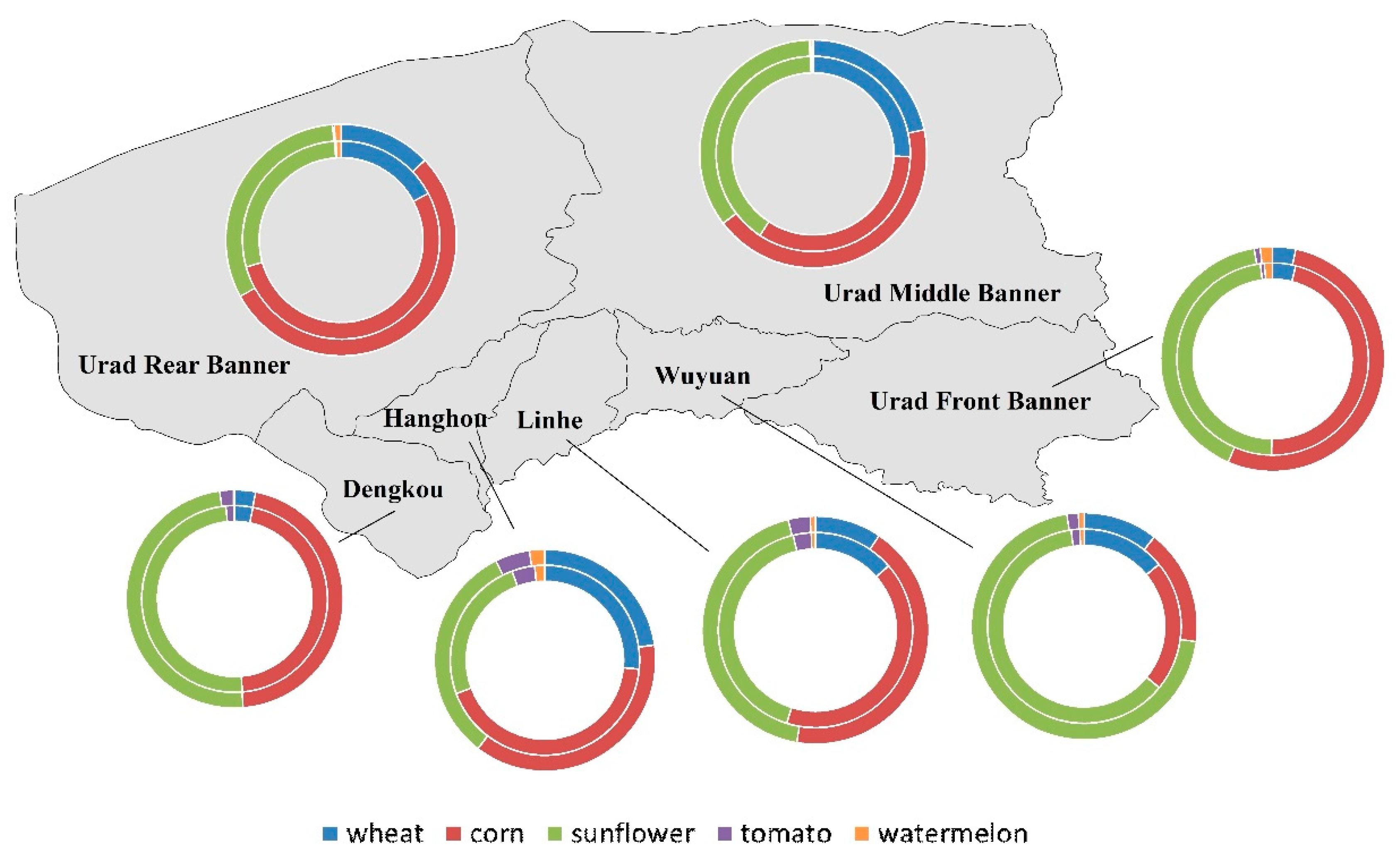
Decisions by Subareas

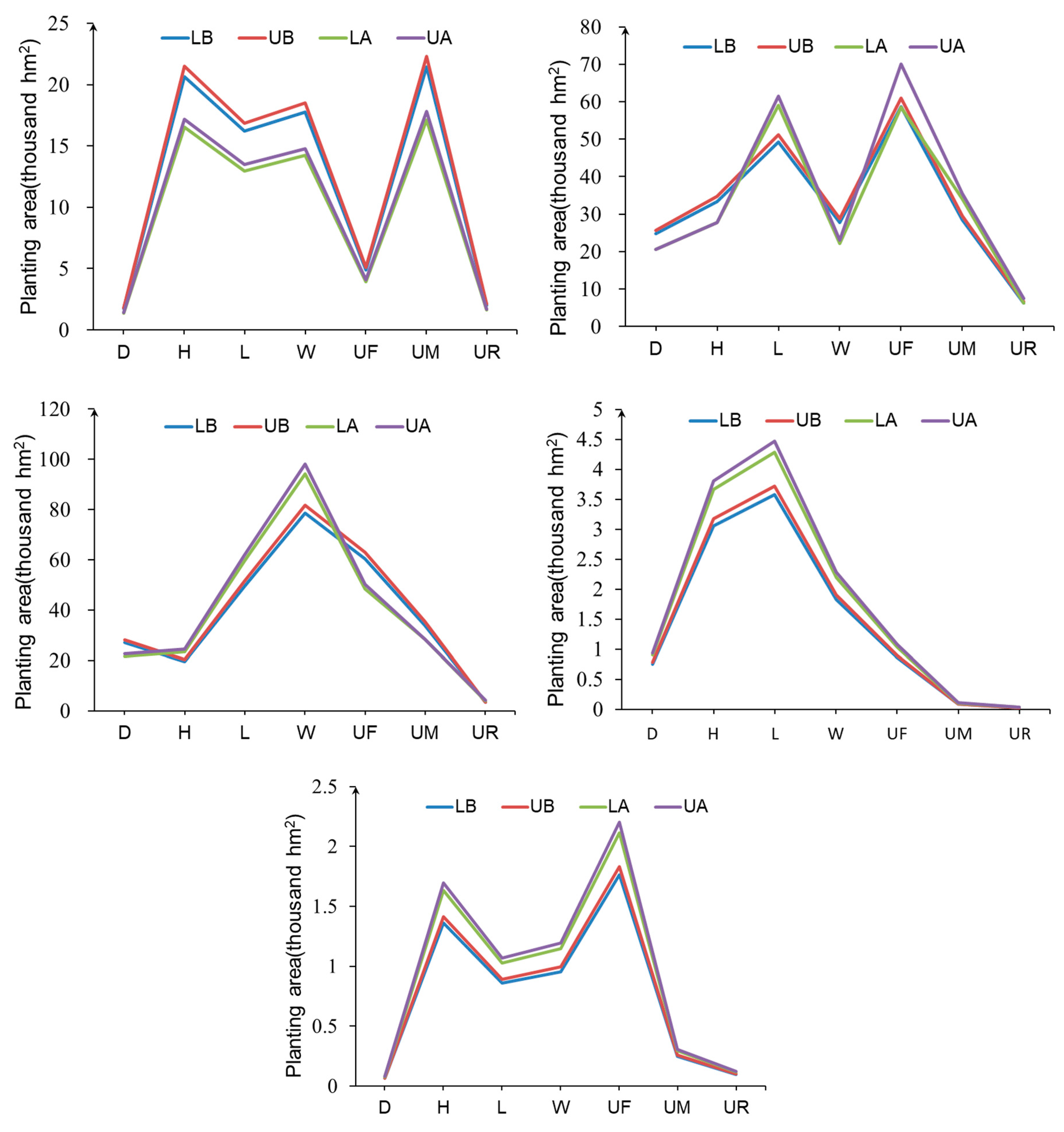
In Dengkou, it is necessary to reduce the planting area of wheat, corn and sunflower, and increase the planting area of tomato and watermelon. Hanghou needs to reduce the proportion of planting area of wheat and corn and increase the proportion of planting area of economic crops like sunflower, tomato, and watermelon. In Linhe, it is necessary to reduce the planting area of wheat and increase the planting area of other crops. Wuyuan needs to reduce the proportion of planting area of wheat and corn and increase the proportion of planting area of economic crops, such as sunflower, tomato, and watermelon. Urad Front Banner needs to reduce the planting area of wheat, corn, and sunflower, and increase the planting area of other crops. Urad Middle Banner needs to reduce the proportion of wheat and sunflower planting area and increase the proportion of corn, tomato and watermelon planting area. Urad Rear Banner needs to reduce the area planted with wheat and increase the area planted by other crops. Adjustment of planting structure in each region of Hetao Irrigation District is shown in Figure 5.

Decisions by Crops

Because the intensity of nitrogen leaching from wheat is relatively large, the planting area in each county has declined under condition of meeting the demand. The corn planting area of Linhe, Urad Front Banner and Urad Rear Banner can be increased at the current level, and other counties should be reduced. According to the optimization results, the planting proportion of sunflower in Hanghou, Wuyuan, and Urad Rear Banner should be increased, and the planting proportion of sunflower in other counties should be reduced. Due to the relatively small intensity of leaching nitrogen, and the small proportion in the planting area of five crops, as an economic crop, the planting area of tomato in each county has increased. The situation of watermelon is similar to that of tomato, and the area planted in each county has increased. Planting structure adjustment for different crops is shown in Figure 6.

4.4.2. Discussion

For the entire Hetao Irrigation District, the optimized wheat planting area decreased, and the planting areas of corn, sunflower, tomato, and watermelon increased. The grey water footprint of wheat production in seven counties of the Hetao Irrigation District decreased by 2.52 × 10⁶ m³, whereas those of corn, sunflower, tomato, and watermelon production increased by 49.8, 192.7, 68.8, and 28.5 × 10³ m³, respectively. The economic benefit loss due to the reduction of wheat planting area was 116 million Yuan, while the economic benefits of corn, sunflower, tomato, and watermelon increased by 123, 309, 709 and 111 million Yuan, respectively. The total water requirement of wheat in the Hetao Irrigation District decreased by 91.6 × 10⁶ m³, and the irrigation water of corn, sunflower, tomato, and watermelon increased by 19.27, 20.29, 5.82, and 2.19 × 10⁶ m³, respectively. It is not difficult to see that the grey water footprint generated by the production of wheat is relatively large, that is, the negative impact on the environment is serious, and the net benefit of crop production is not significant. The grey water footprints generated from economic crops, such as sunflower, tomato, and watermelon are small, but the economic benefits are high, and the water consumption is less. Therefore, under the premise of ensuring demand, appropriately reducing the proportion of wheat and increasing the proportion of economic crops, such as sunflower, will have a positive impact on both economic benefits and environmental soundness. The economic benefits of crops in Dengkou County have declined, economic compensation policies should thus be adopted there. With the aid of the developed model, decision makers can rationally use agricultural water and soil resources with reference to the optimal planting structure, leading to enhanced efficiency of the entire production system through generating the most possible economic benefits with the least possible negative impacts on the environment.

5. Conclusions

In this paper, an agricultural water management model based on grey water footprint was established to deal with the optimization of ratio and uncertainty in pollutant migration and transformation. The model used the interval programming method to tackle uncertain factors associated with hydrology, economics, and technologies. It also included the grey water footprint theory to measure the negative effects of nitrogen leaching during crop production on the ecological environment. The model was applied in the Hetao Irrigation District. Compared with the current planting area, the optimized results showed that the economic benefits from a unit grey water footprint reached maximum which meant the whole system was most efficient. Thirty-four thousand and four hundred m³ grey water would be reduced for every 100 million Yuan of economic benefit. Through adjusting the planting structure, the economic benefits of crops could be increased, whereas the negative effects on the environment during crop production and the consumption of irrigation water could be reduced. Compared to the single-objective model, which only took economic benefit into account, the interval fractional model that compromised more factors would merely moderately reduce the economic benefit. At the same time, as the efficiency of the system associated with the interval fractional model was greater, it could create more economic benefits with the same cost of eco-environmental impairments. The model could provide a decision support tool for the optimization of planting structure and agricultural water use in Hetao and other similar irrigation areas.

In the future, the model can be improved through enhancing the comprehensiveness of constraints. In addition, the quality of data can be consistently improved through more advanced data acquisition techniques and software. Besides, more contaminants and the migration and transformation of contaminants among different water bodies can be involved in the determination of the grey water footprint.

References

1. Carvalho, F.P.; Carvalho, F.D.P. Agriculture, pesticides, food security and food safety. Environ. Sci. Policy 2006, 9, 685–692. [Google Scholar] [CrossRef]
2. Pastori, M.; Udias, A.; Bouraoui, F.; Bidoglio, G. A Multi-Objective Approach to Evaluate the Economic and Environmental Impacts of Alternative Water and Nutrient Management Strategies in Africa. J. Environ. Inform. 2017, 29, 16–28. [Google Scholar] [CrossRef]
3. Foley, J.A.; Ramankutty, N.; Brauman, K.A.; Cassidy, E.S.; Gerber, J.S.; Johnston, M.; Mueller, N.D.; O’Connell, C.; Ray, D.K.; West, P.C.; et al. Solutions for a cultivated planet. Nature 2011, 478, 337–342. [Google Scholar] [CrossRef] [PubMed] [Green Version]
4. Marinov, I.; Marinov, A.M. A Coupled Mathematical Model to Predict the Influence of Nitrogen Fertilization on Crop, Soil and Groundwater Quality. Water Resour. Manag. 2014, 28, 5231–5246. [Google Scholar] [CrossRef]
5. Kapsi, M.; Tsoutsi, C.; Paschalidou, A.; Albanis, T. Environmental monitoring and risk assessment of pesticide residues in surface waters of the Louros River (N.W. Greece). Sci. Total. Environ. 2019, 650, 2188–2198. [Google Scholar] [CrossRef]
6. Torrentó, C.; Prasuhn, V.; Spiess, E.; Ponsin, V.; Melsbach, A.; Lihl, C.; Glauser, G.; Hofstetter, T.B.; Elsner, M.; Hunkeler, D. Adsorbing vs. Nonadsorbing Tracers for Assessing Pesticide Transport in Arable Soils. Vadose Zone J. 2018, 17, 1–18. [Google Scholar] [CrossRef]
7. Li, W.; Bao, Z.; Huang, G.H.; Xie, Y.L. An Inexact Credibility Chance-Constrained Integer Programming for Greenhouse Gas Mitigation Management in Regional Electric Power System under Uncertainty. J. Environ. Inform. 2018, 31, 111–122. [Google Scholar] [CrossRef]
8. Badiozamani, M.M.; Ben-Awuah, E.; Askari-Nasab, H. Mixed Integer Linear Programming for Oil Sands Production Planning and Tailings Management. J. Environ. Informatics 2019, 33, 96–104. [Google Scholar] [CrossRef]
9. Xue, Q.; Yang, X.; Wu, J.; Sun, H.; Yin, H.; Qu, Y. Urban Rail Timetable Optimization to Improve Operational Efficiency with Flexible Routing Plans: A Nonlinear Integer Programming Model. Sustainability 2019, 11, 3701. [Google Scholar] [CrossRef]
10. Li, Y.P.; Huang, G.H.; Cui, L.; Liu, J. Mathematical Modeling for Identifying Cost-Effective Policy of Municipal Solid Waste Management under Uncertainty. J. Environ. Inform. 2019, 34, 55–67. [Google Scholar]
11. Dai, C.; Cai, Y.P.; Lu, W.T.; Liu, H.; Guo, H.C. Conjunctive Water Use Optimization for Watershed-Lake Water Distribution System under Uncertainty: A Case Study. Water Resour. Manag. 2016, 30, 4429–4449. [Google Scholar] [CrossRef]
12. Sun, L.; Li, C.; Cai, Y.; Wang, X. Interval Optimization Model Considering Terrestrial Ecological Impacts for Water Rights Transfer from Agriculture to Industry in Ningxia, China. Sci. Rep. 2017, 7, 3465. [Google Scholar] [CrossRef] [PubMed]
13. Segura, M.; Maroto, C.; Ginestar, C.; Segura, B. Optimization Models to Improve Estimations and Reduce Nitrogen Excretion from Livestock Production. Sustainability 2018, 10, 2362. [Google Scholar] [CrossRef]
14. Singh, A. Simulation–optimization modeling for conjunctive water use management. Agric. Water Manag. 2014, 141, 23–29. [Google Scholar] [CrossRef]
15. Zhang, Z.-Y.; Ma, H.-Y.; Li, Q.-G.; Wang, X.; Feng, G.-X. Agricultural planting structure optimization and agricultural water resources optimal allocation of Yellow River Irrigation Area in Shandong Province. Desalin. Water Treat. 2013, 52, 2750–2756. [Google Scholar] [CrossRef]
16. Zhang, D.M.; Liang, X.J.; Li, Q.W.; Yang, X.H. Study on Model with Multi-Objective Optimization of Planting Structure in Irrigation Area. Yellow River 2013, 35, 91–93. [Google Scholar]
17. Zhu, H.; Huang, W.; Huang, G. Planning of regional energy systems: An inexact mixed-integer fractional programming model. Appl. Energy 2014, 113, 500–514. [Google Scholar] [CrossRef]
18. Tofallis, C. Fractional Programming: Theory, Methods and Applications. J. Oper. Res. Soc. 2017, 49, 895. [Google Scholar] [CrossRef]
19. Cui, H.; Guo, P.; Li, M. Interval fractional programming optimization model for irrigation water allocation under uncertainty. J. China Agric. Univ. 2018, 23, 111–121. [Google Scholar]
20. Guo, P.; Chen, X.; Li, M.; Li, J. Fuzzy chance-constrained linear fractional programming approach for optimal water allocation. Stoch. Environ. Res. Risk Assess. 2013, 28, 1601–1612. [Google Scholar] [CrossRef]
21. Wu, P.; Zhao, X.; Cao, X.; Hao, S. Status and thoughts of Chinese "agricultural north-to-south water diversion virtual engineering". Trans. Chin. Soc. Agric. Eng. 2010, 26, 1–6. [Google Scholar]
22. Hoekstra, A.Y.; Chapagain, A.K.; Aldaya, M.M.; Mekonnen, M.M. The Water Footprint Assessment Manual: Setting the Global Standard; Routledge: London, UK, 2011. [Google Scholar]
23. Borsato, E.; Galindo, A.; Tarolli, P.; Sartori, L.; Marinello, F. Evaluation of the Grey Water Footprint Comparing the Indirect Effects of Different Agricultural Practices. Sustainability 2018, 10, 3992. [Google Scholar] [CrossRef]
24. Mekonnen, M.M.; Hoekstra, A.Y. The green, blue and grey water footprint of crops and derived crop products. Hydrol. Earth Syst. Sci. 2011, 15, 1577–1600. [Google Scholar] [CrossRef] [Green Version]
25. Cao, L.; Wu, P.; Zhao, X.; Wang, Y. Evaluation of grey water footprint of grain production in Hetao Irrigation District, Inner Moreongolia. Trans. Chin. Soc. Agric. Eng. 2014, 30, 63–72. [Google Scholar]
26. Cai, C.; Xia, J.X.; Ren, H.T. Blue water oriented optimization of plantation industry in Xinjiang. Res. Agric. Modern. 2015, 36, 265–269. [Google Scholar]
27. Xu, M.; Li, C.; Wang, X.; Cai, Y.; Yue, W. Optimal water utilization and allocation in industrial sectors based on water footprint accounting in Dalian City, China. J. Clean. Prod. 2018, 176, 1283–1291. [Google Scholar] [CrossRef]
28. Galán-Martín, Á.; Vaskan, P.; Antón, A.; Esteller, L.J.; Guillén-Gosálbez, G. Multi-objective optimization of rainfed and irrigated agricultural areas considering production and environmental criteria: A case study of wheat production in Spain. J. Clean. Prod. 2017, 140, 816–830. [Google Scholar]
29. Ozdemir, M.S.; Saaty, T.L. The unknown in decision making. Eur. J. Oper. Res. 2006, 174, 349–359. [Google Scholar] [CrossRef]
30. Padilla, F.M.; Gallardo, M.; Manzano-Agugliaro, F. Global trends in nitrate leaching research in the 1960–2017 period. Sci. Total. Environ. 2018, 643, 400–413. [Google Scholar] [CrossRef]
31. Ter Steege, M.W.; Stulen, I.; Mary, B.; Lea, P.J.; Morot-Gaudry, J.-F. Nitrogen in the Environment; Springer: Basel, Switzerland, 2001; pp. 379–397. [Google Scholar]
32. Cameron, K.; Di, H.; Moir, J. Nitrogen losses from the soil/plant system: A review. Ann. Appl. Boil. 2013, 162, 145–173. [Google Scholar] [CrossRef]
33. Wang, D.Y.; Li, J.B.; Ye, Y.Y.; Tan, F.F. An Improved Calculation Method of Grey Water Footprint. J. Nat. Res. 2015, 30, 2120–2130. [Google Scholar]
34. Chukalla, A.D.; Krol, M.S.; Hoekstra, A.Y. Grey water footprint reduction in irrigated crop production: Effect of nitrogen application rate, nitrogen form, tillage practice and irrigation strategy. Hydrol. Earth Syst. Sci. 2018, 22, 3245–3259. [Google Scholar] [CrossRef]
35. Xu, W.; Cai, Y.; Rong, Q.; Yang, Z.; Li, C.; Wang, X. Agricultural non-point source pollution management in a reservoir watershed based on ecological network analysis of soil nitrogen cycling. Environ. Sci. Pollut. Res. 2018, 25, 9071–9084. [Google Scholar] [CrossRef] [PubMed]
36. Feng, Z.Z.; Wang, X.K.; Feng, Z.W.; Liu, H.Y.; Li, Y.L. Influence of autumn irrigation on soil N leaching loss of different farmlands in Hetao irrigation district, China. Acta Eco. Sinica 2003, 23, 2027–2032. [Google Scholar]
37. Hu, Y.T.; Liao, Q.J.H.; Wang, S.W.; Yan, X.Y. Statistical Analysis and Estimation of N Leaching from Agricultural Fields in China. Soils 2011, 43, 19–25. [Google Scholar]
38. OuYang, W.; Guo, B.B.; Zhang, X.; Hao, F.H.; Sun, M.Z.; Huang, H.B. Transfer characteristics of soil nitrogen in northern typical irrigation area under different irrigation periods. Chin. Environ. Sci. 2013, 33, 123–131. [Google Scholar]
39. Fan, Y.R. A Robust Two-Step Method for Solving Interval Linear Programming Problems within an Environmental Management Context. J. Environ. Informatics 2012, 19, 1–9. [Google Scholar] [CrossRef]
40. Tan, Q.; Huang, G.H.; Cai, Y. Radial-interval linear programming for environmental management under varied protection levels. J. Air Waste Manag. Assoc. 2010, 60, 1078–1093. [Google Scholar] [CrossRef] [PubMed]
41. Tan, Q.; Huang, G.H.; Cai, Y.P. A Fuzzy Evacuation Management Model Oriented Toward the Mitigation of Emissions. J. Environ. Informatics 2015, 25, 117–125. [Google Scholar] [CrossRef] [Green Version]
42. Tan, Q.; Huang, G.H.; Wu, C.; Cai, Y.; Yan, X. Development of an Inexact Fuzzy Robust Programming Model for Integrated Evacuation Management under Uncertainty. J. Urban Plan. Dev. 2009, 135, 39–49. [Google Scholar] [CrossRef]
43. Huang, G.H.; Loucks, D.P. An inexact two-stage stochastic programming model for water resources management under uncertainty. Civ. Eng. Environ. Syst. 2000, 17, 95–118. [Google Scholar] [CrossRef]
44. Rong, Q.; Cai, Y.; Chen, B.; Yue, W.; Yin, X.; Tan, Q. An enhanced export coefficient based optimization model for supporting agricultural nonpoint source pollution mitigation under uncertainty. Sci. Total. Environ. 2017, 580, 1351–1362. [Google Scholar] [CrossRef] [PubMed]
45. Hladík, M. Generalized linear fractional programming under interval uncertainty. Eur. J. Oper. Res. 2010, 205, 42–46. [Google Scholar] [CrossRef]
46. Dong, C.; Huang, G.; Tan, Q. A robust optimization modelling approach for managing water and farmland use between anthropogenic modification and ecosystems protection under uncertainties. Ecol. Eng. 2015, 76, 95–109. [Google Scholar] [CrossRef]
47. LINGO and Optimization Modeling. Available online: https://www.lindo.com/index.php/products/lingo-and-optimization-modeling (accessed on 18 September 2019).
48. Du, J.; Yang, P.; Li, Y.; Ren, S.; Wang, Y.; Li, X.; Su, Y. Effect of different irrigation seasons on the transport of N in different types farmlands and the agricultural no-point pollution production. Trans. Chin. Soc. Agric. Eng. 2011, 27, 66–74. [Google Scholar]
49. China Agricultural Information. Available online: http://www.agri.cn (accessed on 18 September 2019).
50. Chang, C.L.; Yang, S.Q.; Sun, L.Y.; Liu, D.P. The Relationship between Groundwater Depth and TN in Hetao Irrigation Area during the irrigation and Non-irrigation Period. J. Shenyang Agric. Univ. 2015, 46, 463–470. [Google Scholar]
51. Surface Water Environmental Quality Standard (GB3838-2002); Standards Press of China: Beijing, China, 2002.
52. Groundwater Quality Standard (GB/T14848-93); Standards Press of China: Beijing, China, 1993.
53. Zhang, Y.X.; Shi, X.Y. Groundwater Hydrology; China Water & Power Press: Beijing, China, 1998; p. 162. [Google Scholar]
54. Li, D.B.; Zhang, Q.; Song, X. Present situation of groundwater trinitrogen pollution and main nitrogen removal methods. Environ. Sust. Develop. 2009, 35–37. [Google Scholar] [CrossRef]
55. Park, Y.-C. Cost-effective optimal design of a pump-and-treat system for remediating groundwater contaminant at an industrial complex. Geosci. J. 2016, 20, 891–901. [Google Scholar] [CrossRef]
56. Global Mineral Resources Network. Available online: http://www.worldmr.net (accessed on 18 September 2018).
57. Li, J.F.; Su, X.L. A Multi-objective Optimization Model for Planting Structure Based on the Subdivision of Virtual Water. J. Irrig. Drain. 2013, 32, 126–129. [Google Scholar]
Figure 1. Agrochemical transfer process.
Sustainability 11 05567 g001
Figure 2. Technical framework of the developed model.
Sustainability 11 05567 g002
Figure 3. Study area.
Sustainability 11 05567 g003
Figure 4. Comparison of overall situation of Hetao Irrigation District before and after optimization. Note: LB: Lower bound before optimization; UB: Upper bound before optimization; LA: Lower bound after optimization; UA: Upper bound after optimization; WH: Wheat; C: Corn; S: Sunflower; T: Tomato; WM: Watermelon.
Sustainability 11 05567 g004
Figure 5. Adjustment of Crop Planting Structure in each region of Hetao Irrigation District. Note: The inner layers of the circle are planting areas before optimization; the outer layers of the circle are planting areas after optimization.
Sustainability 11 05567 g005
Figure 6. Planting structure adjustment for different crops. Note: LB: Lower bound before optimization; UB: Upper bound before optimization; LA: Lower bound after optimization; UA: Upper bound after optimization; D: Dengkou County; H: Hangjinhou Banner; L: Linhe District; W: Wuyuan County; UF: Urad Front Banner; UM: Urad Middle Banner; UR: Urad Rear Banner.
Sustainability 11 05567 g006