Abstract
Pedestrian–vehicle collision is an important component of traffic accidents. Over the past decades, it has become the focus of academic and industrial research and presents an important challenge. This study proposes a modified Driving Safety Field (DSF) model for pedestrian–vehicle risk assessment at an unsignalized road section, in which predicted positions are considered. A Dynamic Bayesian Network (DBN) model is employed for pedestrian intention inference, and a particle filtering model is conducted to simulate pedestrian motion. Driving data collection was conducted and pedestrian–vehicle scenarios were extracted. The effectiveness of the proposed model was evaluated by Monte Carlo simulations running 1000 times. Results show that the proposed risk assessment approach reduces braking times by 18.73%. Besides this, the average value of TTC−1 (the reciprocal of time-to-collision) and the maximum TTC−1 were decreased by 28.83% and 33.91%, respectively.
1. Introduction
Pedestrians are a vulnerable group in road traffic accidents. The Annual Statistical Report for Road Traffic Accidents in China showed that pedestrians accounted for 27.11% of the total number of traffic fatalities and 16.72% of the injured in 2017 [1]. Further, pedestrian accidents have also been recognized as an important challenge for emerging autonomous driving technologies. In March 2018, a pedestrian died in a collision with a self-driving Uber vehicle in Arizona, USA, which was the first pedestrian death in the world caused by an unmanned vehicle. Some researchers have found that the majority of traffic accidents could be prevented if a vehicle was able to recognize risk one second in advance. Therefore, risk assessment is of great significance for pedestrian collision avoidance in intelligent vehicles.
Many researchers have attempted to address this issue. Generally, risk assessment includes two types of typical methods in the post-crash stage and pre-crash stage. In the post-crash stage, road traffic risk assessments are generally measured on the basis of historical accident data [2,3] and represented as the indexes of road safety or relative accident rates obtained using statistical models such as accident regression analyses [4,5]. For example, Hojjati-Emami et al. [6] determined the causes of pedestrian–vehicle accidents on roads using a fault tree model. However, slight collisions are generally not included in traffic accident records, and traffic risk analysis methods that are based on previous accident data have low adaptability and accuracy limitations. In the pre-crash stage, classification is proposed on two levels—physics-based models and potential field-based theories—which will be introduced as following. Physics-based models are risk assessment methods which focus on different longitudinal lateral vehicle motion scenarios and directions. They are most commonly used in longitudinal analyses, such as the time-to-collision (TTC), inverse of time-to-collision (TTCi), deceleration rate to avoid a crash (DRAC) [7,8,9], and lateral analyses, such as the car’s current position (CCP), time-to-lane-cross (TLC), and the variable rumble strip (VRBS) [10,11,12]. However, in real traffic environments, traffic risks are continuous variables that cannot be artificially classified into longitudinal or lateral directions.
Potential field-based methods for road traffic risk assessments, which have been widely used in obstacle avoidance and path planning for intelligent vehicles in recent years, are able to overcome the aforementioned problems because of their advantages in terms of environmental description. In 1986, Krogh et al. [13] firstly applied the potential field theory to the perception of the surrounding environment of a robot. Gravity was used to indicate the walkable area, and repulsive force indicated the non-walking area. This was mainly used for the path planning decisions of a robot. In 2012, Hsu et al. [14] introduced the concept of the gravitational field to establish a car-following model based on Krogh’s research. Gravity and repulsive forces were applied to model the lateral and longitudinal behavior of the vehicle, and data calibration was performed from simple experiments. In 1994, Reichardt et al. [15] compared the vehicles in a traffic environment to virtual electronic vehicles, and built a vehicle-centered power field combined with vehicle information, obstacle information, and traffic rules. The system was used to realize the horizontal and vertical control in intelligent vehicles on expressways. Simulation experiments were conducted to verify the validity and practicability of the method. However, although the theory was in line with the actual situation to a certain extent, there were still many realistic scenarios that could not be matched. To solve the problem, Tsourveloudis et al. [16] combined the electrostatic potential field theory with two-layer fuzzy logic reasoning. The environmental road network was analogized to a resistance network, in which each vehicle generated an electrostatic potential field. The optimal path of the vehicle was planned by the current in the network, thereby realizing the automatic path planning of an intelligent vehicle in a dynamic environment. Sattel et al. [17] combined potential field with elastic order from the field of robotics. The elastic order was used to calculate the minimum path in the potential field, in order to plan a vehicle path and avoid falling into the local optimum. The potential field was used to model the lane centerline and lane boundary for collision avoidance. The theory could effectively distinguish between static objects and dynamic objects, and also adapted to the operating characteristics of different drivers through parameter control.
In 2013, Matsumi et al. [18] examined an autonomous collision avoidance system based on the electric braking torque in electric vehicles. In the system, the braking maneuver intensity was determined using potential field theory, which considered the potential hazards because of occlusions in the intersection. Raksincharoensak et al. [19] proposed a virtual spring model that connected a vehicle and pedestrian, to determine the potential field in unsigned intersections with poor visibility. In the same year, Ni Daiheng et al. [20] proposed the field theory of a microscopic traffic model, which was mainly applied to the car-following model. The difference between these theories was that Professor Ni forwarded the vehicle along the lane as a free fall of the object. The vehicle was subjected to the gravitational force brought about by the advancement, the repulsive force brought by the surrounding vehicles, and the repulsive force caused by the difference between the current speed of the vehicle and the driver’s desired speed. Hence, a potential field was formed. The vehicle moved along the lowest point in the potential field map. The theory effectively conforms to the behavioral habits of real drivers; however, it is limited to scene restrictions and does not apply to scenes in which pedestrians interact with cars. Based on Ni Daiheng’s theory, Wang et al. [21,22] constructed a unified Driving Safety Field (DSF) model that included the following: (1) a potential field, which was determined by static objects on the roads, such as a roadblock; (2) a kinetic field, which was determined by the moving objects on the road, such as vehicles and pedestrians; and (3) a behavior field, which was determined by the individual driver characteristics. Rasekhipour et al. [23] applied the artificial potential field method to path planning, obstacle avoidance, and road traffic risk assessment in intelligent vehicles. Different potential functions were assigned to different types of obstacles and road structures. Path was planned based on these potential functions, and vehicle collision avoidance was achieved combined with the planning path and vehicle dynamics constraints. However, the calibration of the parameters is very complicated. To simplify parameter calibration, Zheng et al. [24] developed a model based on equivalent force, which calculated the road traffic risk field in different directions. In all these researches, the road traffic risk was quantified and presented as a distribution in a potential risk map, in which the value of potential energy denoted the road traffic risk level. In this study, DSF is chosen for risk assessment because of its ability to consider two-dimensional risk.
However, the potential field-based method for vehicle risk assessment relies on sensor detection information and causes unnecessary or lacking braking occasionally. It seriously hinders traffic safety. For example, a pedestrian beyond warning range may come into the range and have a crash soon after. A pedestrian who makes the safety assistance system emit an alarm may take no risk for a vehicle because of the change of relative motion. Furthermore, vehicles and two-wheelers are limited by kinematics and dynamics and could not change direction and velocity immediately. Pedestrians are different from them in this term. A pedestrian could do a series of actions consisting of starting, changing his/her direction and stopping in a very short time step. Moreover, frequent brakings relying on pedestrian information from sensor detection would reduce passengers’ driving comfort and increase energy consumption. Therefore, it is meaningful to take pedestrians’ motion intentions into consideration and predict their trajectories for active risk assessment.
Contributions of this paper could be as follows:
- (1)
- A system of risk assessment for pedestrian–vehicle collisions is proposed.
- (2)
- The intention of pedestrian crossing is considered in trajectory prediction model.
- (3)
- The predicted information of pedestrian is applied to DSF for risk assessment.
The remainder of this paper is organized as follows. In Section 2, intention inference process based on Dynamic Bayesian Network (DBN), and the motion prediction with particle filtering are employed for pedestrian trajectory prediction. In Section 3, a modified DSF which combines with prediction is developed for risk assessment. In Section 4, a data collection and parameters calibrations are introduced, after which the effectiveness of the proposed model is verified by conducting Monte Carlo simulation experiments 1,000 times in pedestrian–vehicle collision scenarios. Section 5 provides the discussion and concludes the paper.
2. Overview of Proposed System
In this paper, the system is divided into five parts. A block diagram of overview system is shown in Figure 1.
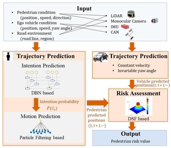
Figure 1.
Block diagram of the proposed system. (LiDAR: Light Detection and Ranging; IMU: Inertial Measurement Unit; CAN: Controller Area Network; DBN: Dynamic Bayesian Network; DSF: Driving Safety Field).
The first block is an input module. Information on pedestrians, vehicles, and road environments is collected from sensors including LiDAR (Light Detection and Ranging), monocular cameras, IMU (Inertial Measurement Unit) and CAN (Controller Area Network). A data-collecting scenario is set at unsignalized roads section in campus, where the pedestrians may walk/cross frequently and pedestrian–vehicle accidents are more likely to occur.
The second block is the pedestrian trajectory prediction module. A pedestrian’s motion features and environmental features are incorporated in a graphical model of DBN, and the crossing-intention of a pedestrian can be estimated through the probabilistic reasoning. A particle filtering is used to forecast a pedestrian’s trajectories, combining with the predicted motion intention.
The third block is vehicle trajectory prediction. Since the research of this paper serves for intelligent vehicle decisions, vehicle trajectories are predicted under the assumption that the vehicle is driven at a constant velocity and invariable yaw angle. Speed changing from decision changes under future pedestrian–vehicle interactions is not considered.
The fourth piece is risk assessment. A modified DSF model was proposed. Predicted trajectories of pedestrians and vehicles are set as input. Behrman equation is defined considering the uncertainties of predicted positions.
Finally, the pedestrian risk value is output to serve the intelligent vehicle decisions.
3. Pedestrian Trajectory Prediction Model
Many novel methods have been proposed for pedestrian behavior modeling and prediction. Mamun et al. [25] studied the effects of pedestrian crossing motion using pedestrian safety interventions and demographic data. Zhou et al. [26,27] used social force model to describe pedestrian collision avoidance patterns, and decision process with considering the impact of PFG (pedestrian flash green) signal on pedestrian crossing motion. In other methods, pedestrian prediction is based on many predecessor features: relative position of pedestrians, speed, pedestrian posture, and depth parallax map and road structure [28,29,30]. However, in most studies, neither pedestrian nor environmental information have been considered. Therefore, this paper considers pedestrian condition, ego vehicle condition, and road environment, with pedestrian trajectory prediction being divided into an intention inference process and a motion prediction process.
3.1. Intention Prediction
A DBN is employed to combine qualitative intentions with additional context information. The intent-related position, motion, and feature details are regarded as hidden variables related to observables, which are variables collected from vehicle equipment.
As shown in Figure 2, hidden variables are selected as pedestrian intent node , which has two possible intentions: crossing the road and not crossing the road. Node is set as an aggregation of the observables from vehicle sensors, and node is set as an aggregation of the hidden variables in a pedestrian’s mind [31].
where is the pedestrian velocity orientation, is the longitudinal distance from pedestrian to ego vehicle, and is the lateral distance from pedestrian to the vehicular road curb. In the hidden variable aggregation , denotes whether a pedestrian needs to cross, which is related to velocity orientation; denotes whether a pedestrian feels any danger when crossing; denotes whether a pedestrian is located on a vehicle road region at which it is possible to cross; , and are discrete variables; and , are continuous variables.
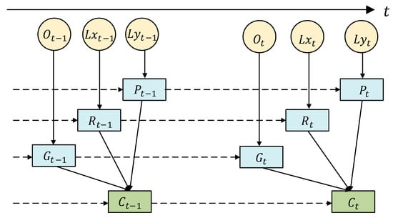
Figure 2.
The DBN-based model for pedestrian intent inference from time step t − 1 to t. Intent (shaded rectangle) is inferred via implication given hidden variables (rectangle). The observed variables (circle) correspond to the hidden variables severally. DBN: Dynamic Bayesian Network.
, and P are independent of each other, have temporal transition, and accord with conditional probability formula. Therefore, the temporal transition for hidden variables is as follows:
where , , and are the temporal transitions for goal , risk , and position , respectively, from time step t − 1 to t.
The probability relationships are independent of each other and also accord with the conditional probability formula. Therefore, the relationship between the observed variables and the hidden variables could be written as follows:
where ,, and indicate the relationships between , respectively, in the same time step.
accords with a Gaussian distribution with a mean value and a standard deviation ; conforms to a Gamma distribution with a parameter λr; and accords with a Polynomial distribution. The conditional distributions for these observables are chosen, and their empirical distributions and parameters are estimated using maximum likelihood estimation on the training data, which are manually annotated with the context states.
The inference DBN process employs Assumed Density Filtering as the approximate inference method [31] and is divided into the “predict” and “update” steps. Prior probability and posterior probability are then introduced in the inference process, which uses the posterior probability of the previous step as the basis for the “predict” step, for which the prior probabilities and are calculated, after which the prior probability is updated to combined with the observables.
Predict:
Update:
At every time step, the network is updated with all available observables, from which the posterior probability of crossing function is inferred.
3.2. Motion Prediction
A DBN-based model is used for pedestrian decision recognition, in which it is necessary to know where the pedestrian is going to reach in the following time steps. Therefore, a pedestrian motion model is set up by employing a sample-based particle filtering method, with the approximate Bayesian filtering algorithm based on a Monte Carlo simulation. Different from the Kalman filter method, which describes the system using explicit probabilistic model parameters, the particle filtering uses the sample mean of the particle set to estimate the parameters. That is to say, the particle filtering sets discrete particles to simulate the probability density of the variables. The weighting and recursive propagation of its particle set are also based on the Bayesian criterion.
The priori predicted value of the particle state at time t is calculated on the basis of the pedestrian motion equation.
where (9) to (11), respectively, are the equations for the change in pedestrian position, direction, and velocity; is the position of the pedestrian’s absolute coordinates at time step t; is the direction of motion; and is a speed variable without direction at time step t. Therefore, we have , , and . indicates the direction noise for pedestrians who are maintaining their current direction, so as to obtain .
Traditionally, Gaussian functions are usually used for importance sampling in the particle filtering, with the particle importance weight being generally updated by comparing the particle states with the observed true values. However, in this research, as there are no observed prediction values, is set for the weight calculations in consideration of the particle states and crossing probability from the DBN-based intention model.
where and denote whether the particle is in the sidewalk region or the vehicle road region; is the posterior probability for pedestrian crossing-intention; indicates a road crossing; and indicates that there is no crossing decision.
After the weight calculation, some particles are discarded and the remaining particles are normalized using the following formula:
Then, depending on weight size, random re-resampling is employed to obtain a posterior update value for the particle states. The updated particle distribution and the expectation of the next time step will be output.
4. Risk Assessment Model
The DSF is a physical field that denotes the influence of objects on driving safety [22]. In this paper, the objects refer to elements such as vehicles, pedestrians, and cyclists that could collide with vehicles and result in significant losses.
where, is the field strength vector at formed by ego vehicle at that denotes the potential risk to the surroundings of ego vehicle under the prevailing road conditions; is the virtual mass of ego vehicle; is the distance vector between the pedestrian and ego vehicle center of mass; and is the velocity vector of ego vehicle. is directed along the gradient descent direction of the field strength when away from ego vehicle; that is to say, the field strength increases as decreases.
where , , and are undetermined constants greater than 0; is the road width parameter that aims to limit the risk in one lane; is the angle between the direction of and the x-axis; and is the angle between the directions of and . When denotes the same distance, the field strength increases as decreases; that is to say, the potential risk increases; and denotes the gradient descent direction of the field strength . The center of the field is the center mass of ego vehicle, with the field strength being more densely distributed in the forward direction of ego vehicle.
where is the virtual mass of ego vehicle; and are the weight and velocity; is the type such as vehicles, pedestrians, and cyclists; and , and are constants greater than 0, the values of which are determined by the maximum likelihood estimations of the relationships between velocity and accident damage.
where is the field force vector at formed by ego vehicle at that denotes the potential acting force on the surroundings because of ego vehicle under the prevailing road conditions and is the virtual mass of the pedestrian at .
where has the same gradient descent direction as the field strength and is the unit field strength descent.
Because of errors in the pedestrian trajectory prediction with time, is employed as an attenuation coefficient to solve the problem based on the Bellman equation; that is to say, the field force in rear steps is attenuated.
where indicates the new field force vector based on prediction at that is formed by ego vehicle at on the basis of the trajectories in the following predicted steps.
5. Dataset and Experiment
5.1. Data Collection
The data collection equipment is an electrical vehicle, Dongfeng Venucia E30, as shown in Figure 3, which has few vibrations because the internal combustion engine has been replaced by an electrical motor, which, in turn, makes the sensing system more stable and reliable.
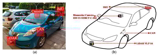
Figure 3.
Data collection vehicle (Dongfeng Venucia E30). Sensors were equipped on the vehicle body and inner. (a) Ego vehicle (Dongfeng Venucia E30), (b) Ego vehicle Hardware structure. (LiDAR: Light Detection and Ranging; IMU: Inertial Measurement Unit; CAN: Controller Area Network)
The vehicle was equipped with a LiDAR (Velodyne VLP-16) in the front of the vehicle body; a monocular camera (IDS UI-5250CP-C-HQ) behind the inside mirror; an IMU in the trunk; and a CAN near the left wheel. A Robot Operating System (ROS) was used to collect and save data from the above sensors. The collecting data were recorded from those sensors, as shown in Table 1. The LiDAR and monocular camera collect information by using the artificial label of the pedestrian and the road environment. Detail sources of collection data are shown in Figure 3. The monocular camera provides an image of road lanes, and the LiDAR returns positions of the target pedestrian and the road edge using artificial labeling from the two-dimensional point cloud image. The vehicle CAN returns information regarding ego vehicle, such as velocity and yaw angle, and the IMU provides information on acceleration rate. The positional ground truth of the pedestrians was obtained using coordinate transformation and calculation. Due to the different frequency of sensors with 10 Hz for LiDAR, 15 Hz for monocular camera, 100 Hz for IMU, and 10 Hz for CAN, the data collection frequency was processed with 10 Hz.

Table 1.
Collection data sources. (LiDAR: Light Detection and Ranging; IMU: Inertial Measurement Unit; CAN: Controller Area Network).
The dataset scenario was an unsigned road section of a university campus. Location is shown in Figure 4, roads with 1186 meters in the Tsinghua University campus. These roads are two-lane roads with sidewalks, no center separation band handrails, and no zebra marking, where pedestrians cross randomly as they need. The maximum vehicle speed limit inside the campus is 30 km/h. They are typical places where pedestrian–vehicle interactions happen. In data collection, senior drivers were employed and drove with natural driving habits. The data applied in this study are shown in Table 2. To calibrate the parameters in the above models, the statistics are classified into ten parts, with eight parts for the training set and two parts for the test set.
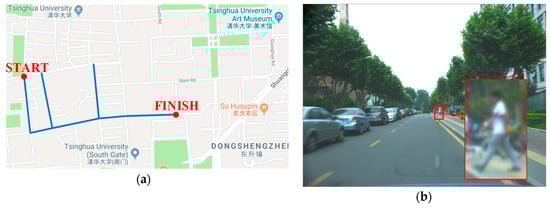
Figure 4.
(a) The road section location for data collection; (b) Actual scenario is a road section of a no-named road in the Tsinghua University campus.
Table 2.
Collection statistics (Unit: Frame; LiDAR: Light Detection and Ranging; IMU: Inertial Measurement Unit; CAN: Controller Area Network).
5.2. Experiment Results
The pedestrian trajectory prediction model was further verified using the test set. Crossing-intention probability was acquired on the basis of DBN intention recognition model; if the probability was below 0.4, it was classified as no pedestrian crossing, and if the probability was over 0.4, it was classified as a pedestrian crossing. Particle filtering was used for the motion prediction based on the intention inference result. One hundred particles were generated for every 0.5 s step, which, in turn, ensured that the trajectory prediction results simulated larger pedestrian behavior change trajectory probabilities. Prediction duration was about 3.0 s of common pedestrian short-term movement prediction at six steps per 0.5 s.
The two test trajectory prediction subscenarios are selected to be shown as follows, in which the blue dots indicate the probable future position set from the results with the color fading with the prediction time, the red dot indicates pedestrian current position; the light blue truth path is the observed trajectory from the database; the white is ego vehicle and its path; the green areas indicate pavements; and the gray areas indicate motorized vehicle lane.
Figure 5 shows the trajectory prediction of pedestrians in the scene of pedestrian crossing. Figure 5a shows that when the pedestrian is moving towards the vertical direction of the road at the speed of 1.41 m/s on the sidewalk with 1.41 m away from the road edge, the inferred probability of pedestrian crossing-intention is 0.81. At this time, the ego vehicle drove ahead at speeds of 6.14 m/s and at the distance of 21.52 m away from the pedestrian. As time goes by, the vehicle approached at speed of natural driving, and pedestrians speed up slightly. The probability of pedestrians crossing increases gradually from 0.81 to 0.92, and the crossing-intention becomes clearer. In the whole prediction process in every 3.0 s, the actual trajectory of pedestrians arriving in the future is in the particles dense area of the prediction trajectory domain, which indicates that the prediction results are effective in line with the real trajectory behavior of pedestrians.
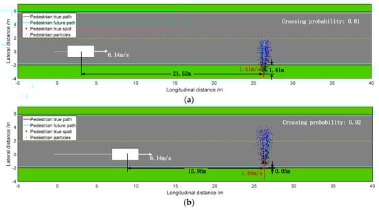
Figure 5.
Crossing case A of trajectory prediction of pedestrian in two subscenarios. (a) t = 0.3 s, when the pedestrian was on the sidewalk. (b) t = 1.0 s, when the pedestrian was on the curb side. Pedestrian trajectory prediction particles are shown in blue, past actual trajectory in red, future actual trajectory in light blue, and vehicle in white.
As shown in Figure 6, the track domain prediction of pedestrians is in the scene of the pedestrian changing direction frequently. As can be seen in Figure 6a, the pedestrian moves along the road in a parallel direction at the speed of 0.75 m/s on the sidewalk, with 0.33 m from the road edge, and the vehicle approaches the pedestrian at the speed of 17.5 km/h and at the distance of 23.31 m from the pedestrian. At this time, the inferred probability of pedestrian crossing-intention is 0.87, indicating that the pedestrian has strong crossing-intention. The actual trajectory shown in the figure is the complete trajectory collected, and the particles prediction is to predict the positions that pedestrian may reach with 6 steps, namely 3.0 s. Therefore, the actual trajectory of pedestrians exceeds the predicted particle swarm over 3.0 s, which is a normal phenomenon. It can be seen from Figure 6b that, when pedestrians enter a motor vehicle lane, the probability of crossing-intention recognition is 1.0, indicating that there is a clear crossing-intention. As time goes by, the pedestrian moved with irregular changes in direction and speed. However, the future pedestrian actual trajectory does not conform to the concentrated area of the particle swarm as in the above scene, but also in the predicted particles field.
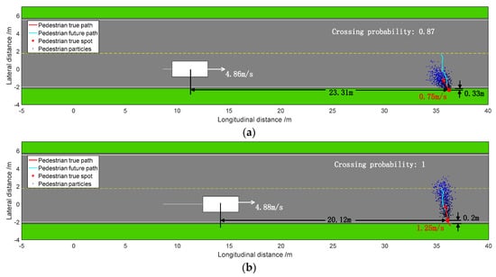
Figure 6.
Crossing case A of trajectory prediction of pedestrian in two subscenarios. (a) t = 0.1 s, when the pedestrian was on the curb side. (b) t = 0.6 s, when the pedestrian was on the road. Pedestrian trajectory prediction particles are shown in blue, past actual trajectory in red, future actual trajectory in light blue, and vehicle in white.
The vehicle head, rather than the physical center, is set as the mass in the field center, and through calibration and from previous research [22], a set of model parameters are determined.
is an undetermined constant greater than 0. depends on the magnitude of the field strength, which is related to scenarios application of DSF. and are also undetermined constants greater than 0. is determined by the relationship between the field strength and , which is the distance vector between the pedestrian and the mass of the field center. depends on the spatial distribution which is influenced by velocity vector of ego vehicle. is an undetermined constant related with the width of the road lane and is determined to compress the lateral width of the field strength and reduce the impact on adjacent lanes. is the weight of ego vehicle and our experimental vehicle (electrical vehicle, Dongfeng Venucia E30), having the weight of 1400.0 kg, and is the weight of the pedestrian. In this research, the average weight of experimental volunteers is 70.0 kg.
, and are constants greater than 0, which are determined by the maximum likelihood estimations of the relationships between velocity and accident damage in formula (17). The velocity and accidents are counted in Table 3.
Table 3.
Speed and accidents in China, 2017 [1].
The power function of formula (17) related to velocity is obtained by fitting the average number of fatalities in each accident. As is presented in formula (22).
Hence, parameters are calibrated and shown in Table 4.
Table 4.
Parameter calibration.
By calculating the field strength of the true pedestrian position at past moment and the position of the predicted particles, a curve of field strength was developed, as shown in Figure 7. The scenario of Figure 5a was selected as an example. At that moment, the vehicle trajectory was predicted under the assumption of driving with constant velocity and invariable yaw angle. It can be clearly seen in the curve that field strength increases with prediction time. The field strength was more dispersive because of particles dispersing with time. The attenuation coefficient was defined considering the uncertainties of trajectory predictions in the modified model. Therefore, the proposed model is able to determine the dangerous tendency of pedestrians in advance.
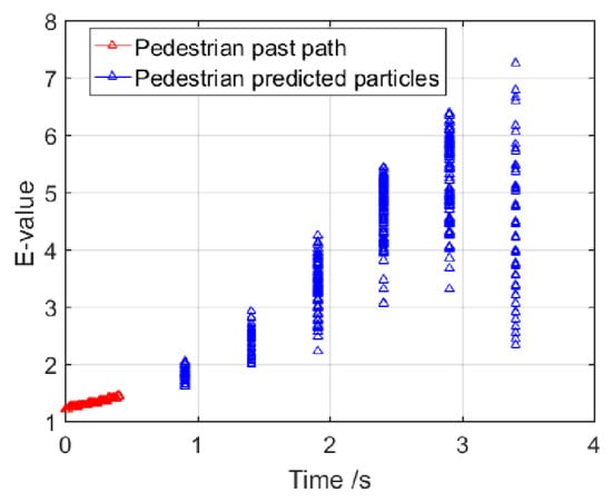
Figure 7.
Field strength of each predicted particles in the scenario.
5.3. Experiment Results and Discussions
To quantitatively compare the potential field with and without prediction, a Monte Carlo experiment is designed to simulate the vehicle driving process based on the artificial potential field braking rule. The braking rule is set such that the vehicle adopted a braking mode to reduce the fixed speed by 1 m/s when the field force calculated using (18) and (21) exceeded the threshold of 50.
In Monte Carlo experiments, the initial ego vehicle position is (U (−2, 2), U (−0.5, 0.5)), and the initial speed is U (5, 8). Therefore, (U (20, 30), U (−4, −2)) is taken as the initial pedestrian position; the initial pedestrian speed is U (0, 2.6); and the initial pedestrian speed direction is U (0, 360). To simulate pedestrian movement, random sampling of the predicted particles is then used as the pedestrian position in the next moment. The higher the field force, the higher the danger. Ego vehicle will brake if the field force exceeds the threshold of 50. To evaluate the safety of these two risk assessment methods, the traditional TTC method is used. Therefore, the TTC values for the two methods are calculated for the simulation process; in this case, the smaller the TTC, the greater the danger. To make the comparison easier to understand, TTC−1 is employed; therefore, in this case, the higher the TTC−1, the greater the danger. For one simulation, the field force , and the TTC values are the two modes shown in Figure 8.
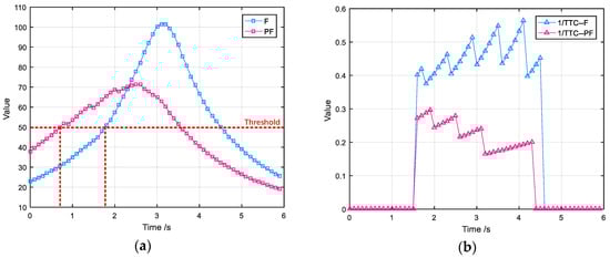
Figure 8.
Comparison of two-field force and TTC−1 in Monte Carlo simulation process. (a) Comparison of the constituents of the two-field force: F is the field force with non-prediction and PF indicates the field force with prediction. (b) Comparison of TTC−1 values relative to the two-field force.
It can be seen from Figure 8a that, in this scenario, the PF field force is higher with prediction than it is with non-prediction at the beginning of the simulation, because the predicted particles have a higher field force value as the pedestrian and ego vehicle are approaching. Because of the same braking rule threshold value, the prediction method lead to ego vehicle braking 1.22 s earlier and more smoothly than without prediction, as can be seen in Figure 8b, where the TTC−1 for the PF is lower than for the F. Earlier braking means that the safety field value drops faster, which reduces sudden vehicle braking. The proposed method also has less braking at only four times when compared with six times in the previous method. To acquire more convincing proof, 1000 Monte Carlo simulations are randomly conducted and the average braking times for the two methods are calculated. The TTC−1 average values and peak values for the simulation are shown in Table 5. As can be seen, the mean braking time for the proposed method is 3.958, which is a decrease of −18.73% over the other method, indicating that vehicle driving is more smooth. To measure the TTC−1 safety index improvements, the mean and mean peak are both chosen and compared with the non-prediction scenario, from which improvements of −28.83% and −33.91% are found.
Table 5.
Comparison of the potential field with non-prediction and with prediction.
6. Conclusions
In this study, we presented a modified DSF model for pedestrian–vehicle risk assessment based on pedestrian’s future trajectory predictions, for which multisensors such as LiDAR and monocular cameras were used to collect scenario data in a real traffic environment. Pedestrian’s motion features, in addition with the environmental features, were incorporated into DBN for inferring pedestrian’s crossing-intentions. Particle filtering was then used for predicting the future trajectories in following 3.0 s with the estimated crossing-intention of the pedestrian. We collected data through a real-world driving experiment in pedestrian–vehicle scenarios. The predicted trajectory uncertainty was defined in our modified DSF model for proactive risk assessment by using an attenuation coefficient that was based on the Bellman equation. Mean braking times, TTC−1 mean, and TTC−1 mean peak were taken as the evaluation index to compare the developed model with a risk assessment model without predictive factors. Monte Carlo simulations were taken 1000 times, from which it was found that our modified DSF model could reduce braking operations by 18.73%. The average values of both TTC−1 and the maximum TTC−1 decreased by 28.83% and 33.91%, respectively. A time-varying risk value is applied to traffic risk assessment. The proposed algorithm could be included as part of the intelligent decisions in Autonomous Vehicles to make them smarter and safer.
Future work intends to improve expansibility and general applicability for the algorithm to enable safe and efficient driving of intelligent vehicles in pedestrian–vehicle scenarios. Cover the following two aspects: one for expanding the database to consider scenarios with different road structures and more pedestrians. Moreover, additional experiments will focus on how to deal with the situation of braking failure caused by algorithm malfunction.
Author Contributions
Conceptualization, R.W.; Methodology, X.Z.; Validation, W.W.; Formal analysis, Y.X. and Z.N.; Data curation, X.Z.; Writing—original draft preparation, R.W.; writing—review and editing, Y.X. and Q.X.; Funding acquisition, Y.X.; Supervision, G.L.
Funding
This research was funded by the National Science Fund for Distinguished Young Scholars, grant number 51625503; the National Natural Science Foundation of China, the Major Project, grant number 61790561; Fundamental Research Funds for the Central Universities, grant number 30917012102 and the open fund for Jiangsu key laboratory of traffic and transportation security (Huaiyin Institute of Technology), grant number TTS2017-02.
Acknowledgments
More importantly, we also want to thank Jianqiang Wang for guidance and providing experimental hardware facilities and platforms. Thanks are extended to Likun Wang, Yougang Bian, Yang Li, and Liu Lu (Tsinghua University, Beijing) for supporting the real vehicle experiments, as well as the anonymous reviewers for their valuable suggestions and comments.
Conflicts of Interest
The authors declare no conflict of interest.
References
- The Ministry of Public Security Traffic Management Bureau. The Annual Statistical Report for Road Traffic Accidents in China (2017); The Ministry of Public Security Traffic Management Bureau: Jiangsu, China, 2018. [Google Scholar]
- Schlögl, M.; Stütz, R. Methodological considerations with data uncertainty in road safety analysis. Accid. Anal. Prev. 2017, 130, 136–150. [Google Scholar] [CrossRef] [PubMed]
- Staton, C.; Vissoci, J.; Gong, E.; Toomey, N.; Wafula, R.; Abdelgadir, J.; Zhao, Y.; Liu, C.; Pei, F.; Zick, B. Correction: Road Traffic Injury Prevention Initiatives: A Systematic Review and Metasummary of Effectiveness in Low and Middle Income Countries. PLoS ONE 2016, 11, e0150150. [Google Scholar] [CrossRef]
- Chen, F.; Wang, J.; Wu, J.; Chen, X.; Zegras, P.C. Monitoring road safety development at regional level: A case study in the ASEAN region. Accid. Anal. Prev. 2017, 106, 437–449. [Google Scholar] [CrossRef] [PubMed]
- Lord, D.; Mannering, F. The statistical analysis of crash-frequency data: A review and assessment of methodological alternatives. Transp. Res. Part A 2010, 44, 291–305. [Google Scholar] [CrossRef]
- Hojjati-Emami, K.; Dhillon, B.S.; Jenab, K. The Stochastic and Integrative Prediction Methodology and Modeling for Reliability of Pedestrian Crossing on Roads. J. Transp. Saf. Secur. 2013, 5, 257–272. [Google Scholar] [CrossRef]
- Qu, X.; Kuang, Y.; Oh, E.; Jin, S. Safety evaluation for expressways: A comparative study for macroscopic and microscopic indicators. J. Crash Prev. Inj. Control 2014, 15, 89–93. [Google Scholar] [CrossRef]
- Ward, J.R.; Agamennoni, G.; Worrall, S.; Bender, A.; Nebot, E. Extending Time to Collision for probabilistic reasoning in general traffic scenarios. Transp. Res. Part C Emerg. Technol. 2015, 51, 66–82. [Google Scholar] [CrossRef]
- Sharifi, M.S.; Stuart, D.; Christensen, K.; Chen, A. Time Headway Modeling and Capacity Analysis of Pedestrian Facilities Involving Individuals with Disabilities. Transp. Res. Rec. 2016, 2553, 41–51. [Google Scholar] [CrossRef]
- Tan, D.; Chen, W.; Wang, H. On the Use of Monte-Carlo Simulation and Deep Fourier Neural Network in Lane Departure Warning. IEEE Intell. Transp. Syst. Mag. 2017, 9, 76–90. [Google Scholar] [CrossRef]
- Sun, C.; Edaram, P.; Ervin, K. Elevated-Risk Work Zone Evaluation of Temporary Rumble Strips. J. Transp. Saf. Secur. 2011, 3, 157–173. [Google Scholar] [CrossRef]
- Wang, J.G.; Lin, C.J.; Chen, S.M. Applying fuzzy method to vision-based lane detection and departure warning system. Expert Syst. Appl. 2010, 37, 113–126. [Google Scholar] [CrossRef]
- Krogh, B.; Thorpe, C.E. Integrated path planning and dynamic steering control for autonomous vehicles. Proceedings of 1986 IEEE International Conference on Robotics and Automation, San Francisco, CA, USA, 7–10 April 1986. [Google Scholar]
- Reichardt, D.; Shick, J. Collision avoidance in dynamic environments applied to autonomous vehicle guidance on the motorway. In Proceedings of the Intelligent Vehicles’ 94 Symposium, Paris, France, 24–26 October 1994. [Google Scholar]
- Tsourveloudis, N.C.; Valavanis, K.P.; Hebert, T. Autonomous vehicle navigation utilizing electrostatic potential fields and fuzzy logic. IEEE Trans. Robot. Autom. 2001, 17, 490–497. [Google Scholar] [CrossRef]
- Sattel, T.; Brandt, T. From robotics to automotive: Lane-keeping and collision avoidance based on elastic bands. Veh. Syst. Dyn. 2008, 46, 597–619. [Google Scholar] [CrossRef]
- Hsu, T.-P.; Weng, G.-Y.; Lin, Y.-J. Conceptual structure of a novel car-following model upon gravita-tional field concept. In Proceedings of the 19th ITS World CongressERTICO-ITS EuropeEuropean Com-missionITS AmericaITS Asia-Pacific, Vienna, Austria, 22–26 October 2012. [Google Scholar]
- Matsumi, R.; Raksincharoensak, P.; Nagai, M. Autonomous Braking Control System for Pedestrian Collision Avoidance by Using Potential Field. IFAC Proc. Vol. 2013, 46, 328–334. [Google Scholar] [CrossRef]
- Raksincharoensak, P.; Akamatsu, Y.; Moro, K.; Nagai, M. Predictive Braking Assistance System for Intersection Safety Based on Risk Potential. IFAC Proc. Vol. 2013, 46, 335–340. [Google Scholar] [CrossRef]
- Ni, D. A unified perspective on traffic flow theory. Part I: The field theory. Appl. Math. Sci. 2013, 7, 37–40. [Google Scholar] [CrossRef]
- Wang, J.; Wu, J.; Li, Y. The Driving Safety Field Based on Driver–Vehicle–Road Interactions. IEEE Trans. Intell. Transp. Syst. 2015, 16, 2203–2214. [Google Scholar] [CrossRef]
- Wang, J.; Wu, J.; Zheng, X.; Ni, D.; Li, K. Driving safety field theory modeling and its application in pre-collision warning system. Transp. Res. Part C Emerg. Technol. 2016, 72, 306–324. [Google Scholar] [CrossRef]
- Rasekhipour, Y.; Khajepour, A.; Chen, S.-K.; Litkouhi, B. A Potential Field-Based Model Predictive Path-Planning Controller for Autonomous Road Vehicles. IEEE Trans. Intell. Transp. Syst. 2017, 18, 1255–1267. [Google Scholar] [CrossRef]
- Zheng, X.; Zhang, D.; Gao, H.; Zhao, Z.; Huang, H.; Wang, J. A Novel Framework for Road Traffic Risk Assessment with HMM-Based Prediction Model. Sensors 2018, 18, 4313. [Google Scholar] [CrossRef]
- Mamun, S.; Caraballo, F.J.; Ivan, J.N.; Ravishanker, N.; Townsend, R.M.; Zhang, Y. Identifying Association between Pedestrian Safety Interventions and Street-Crossing Behavior Considering Demographics and Traffic Context. Available online: https://kopernio.com/viewer?doi=10.1080/19439962.2018.1490369&route=6 (accessed on 23 June 2019).
- Zhou, Z.; Cai, Y.; Ke, R.; Yang, J. A collision avoidance model for two-pedestrian groups: Considering random avoidance patterns. Phys. A Stat. Mech. Appl. 2017, 475, 142–154. [Google Scholar] [CrossRef]
- Zhou, Z.; Zhou, Y.; Pu, Z.; Xu, Y. Simulation of pedestrian behavior during the flashing green signal using a modified social force model. Transp. A Transp. Sci. 2019, 15, 1019–1040. [Google Scholar] [CrossRef]
- Karasev, V.; Ayvaci, A.; Heisele, B.; Soatto, S. Intent-aware long-term prediction of pedestrian motion. In Proceedings of the IEEE International Conference on Robotics & Automation, Stockholm, Sweden, 16–21 May 2016. [Google Scholar]
- Goldhammer, M.; Gerhard, M.; Zernetsch, S.; Doll, K.; Brunsmann, U. Early prediction of a pedestrian’s trajectory at intersections. In Proceedings of the International IEEE Conference on Intelligent Transportation Systems, The Hague, The Netherlands, 6–9 October 2013. [Google Scholar]
- Iryo-Asano, M.; Alhajyaseen, W. Consideration of a Pedestrian Speed Change Model in the Pedestrian–Vehicle Safety Assessment of Signalized Crosswalks. Transp. Res. Procedia 2017, 21, 87–97. [Google Scholar] [CrossRef]
- Kooij, J.F.P.; Flohr, F.; Pool, E.A.I.; Gavrila, D.M. Context-Based Path Prediction for Targets with Switching Dynamics. Int. J. Comput. Vis. 2019, 127, 239–262. [Google Scholar] [CrossRef]


© 2019 by the authors. Licensee MDPI, Basel, Switzerland. This article is an open access article distributed under the terms and conditions of the Creative Commons Attribution (CC BY) license (http://creativecommons.org/licenses/by/4.0/).