Abstract
In order to improve environmental performance, the participation of effective and transparent citizens and governments that help counteract corruption in environmental matters is crucial. In this sense, this work focuses on exploring relationships between e-participation, e-government, the corruption index and environmental performance indicators. To this end, a sample comprising 116 countries from varying geographic regions is used in conjunction with indicators of environmental performance, e-participation, e-government and the corruption index. Through the use of the HJ-biplot and STATIS multivariate statistical techniques, it will be possible to observe the role that these variables play in countries’ behavioural patterns with respect to environmental performance. The results show a correlation between the indicator ‘perception of corruption’ and environmental performance; therefore, the lower the level of corruption, the higher the environmental performance index. We conclude that countries that exhibit more e-participation, lower levels of corruption and better level income are more likely to follow policies and programmes aimed at achieving better environmental performance.
1. Introduction
This research focuses on examining how environmental performance is related to e-government, e-participation and the corruption index. We seek to understand relationships between the different variables and how they explain the similarities and differences between countries, within the context of their level income. We base our study on previous works such as Wang et al. [1] that show the effect of corruption on poor environmental performance; Burakov et al. [2] highlights that corruption and inequality increase environmental degradation and; Aniscenko et al. [3] indicate that the development of e-government is positively related to sustainable development and better governance. Thus, we have selected the indicators e-participation, e-government and corruption to explore these relationships as a whole, using multivariate techniques, all seen from the point of view of the income levels of the countries.
We make a comparison at the country level since the level of development of citizen participation, and environmental sustainability is determined by the different policies that governments develop at the local, regional and national levels. Although the regional contribution differs depending on the level of federalist structure of each country, the role of the state administration and, especially, of local governments is unquestionable in all the countries analysed. The relevance that local policies have over national policies in the inclusion of the opinion of citizens in sustainable development should be noted because a high percentage of society lives in cities, with urban areas being the demarcations used for (i) the carrying out all types of citizen consultations; and (ii) the establishment of policies that allow the design of sustainable cities
To achieve development with environmental sustainability, a set of regulatory, administrative and operational actions is necessary, which must be promoted by the State and local governments; this is known as environmental management [4,5]. In this context, environmental information is fundamental within environmental management processes, since it configures the base that facilitates the quantification and measurement of environmental quality. Several indicators have been implemented in order to understand and manage all sustainability issues. Within these, the Environmental Performance Index (EPI) [6] provides a nationwide indicator of how close countries are to their established environmental policy objectives.
The rapid development of information and communication technologies (ICT) has generated the growth of e-participation, whereby governments use digital tools to boost citizen participation, developing e-government. According to Justice, Melitski and Smith [7], e-governments improve transactions between the government and other agents, changing both the provision of public services and the broader field of interactions between citizens and the government [8]. E-governments allow citizens to take part in democratic institutions and political processes [7,9], producing an image of accessible, transparent, responsible, effective and participatory governance [10]. However, the lack of transparency of online information by institutions exerts a negative influence regarding sustainability [11].
E-participation contributes to the increase and progress of communications between the citizens themselves and the ruling politicians [12] and therefore, in democratic processes [13]. In this sense, e-participation is of vital importance for the development of policies aimed at improving sustainability [14].
Regarding the above, the United Nations [15] notes that governance for sustainable development goes hand-in-hand with national strategic planning to ensure efficiency and transparency. According to Voß et al. [16], environmental and sustainability issues are characterised by their complexity and, as indicated by Renn and Schweizer [17], special attention should be paid to the structure of the participation process in order to achieve the stated objectives.
On the other hand, corruption has become a global problem and compromises governance, transparency and accountability [18], becoming a very worrying problem in developing countries [19]. This is particularly with regard to environmental issues since these are extremely vulnerable to corruption [20,21,22], affecting environmental quality through different routes [23]. In this sense, we ask ourselves, could e-participation and e-governments play an important role in anti-corruption policy and therefore contribute to the improvement of environmental performance?
Environmental performance as a dimension of sustainable development is of great importance to today’s society, which justifies the need to know the interests of citizens and their specific demands in relation to the environment. In this sense, we explore how the environmental development index relates to other variables linked to transparent governments in 116 countries from varying geographical areas. Using a variety of sources, we examine the relationship of the environmental development index with three indicators: e-government, e-participation and corruption index. Also, countries were analyzed according to their income level.
Our objective is to explore how the environmental development index is related to these variables, and if any relationship is clearly stronger; in the same way, we sought to understand the structures underlying the data, specifically to relations between the different indices and how these indices manage to explain the similarities and differences between countries. We also contribute to studies on environmental performance and citizen perception through recently developed multivariate techniques such as HJ-biplot and STATIS.
In terms of previous arguments and empirical evidence, we defend the proposal that countries with higher levels of e-participation, better e-government indicators and lower levels of corruption generally have better environmental performance indicators and that these indicators behave according to the economic level of the countries. Considering the findings of these previous studies, we hypothesised that e-participation, e-government, corruption index and income level are related to the environmental performance index. These variables, therefore, were addressed in this study from the perspective that a better understanding of the possible relationships of these variables on environmental performance could be used as the basis for developing specific studies of these relationships, leading to improved levels of environmental performance.
2. Materials and Methods
2.1. Population and Sample
To achieve the objective of our work, we considered the 236 countries reported in the EPI report for the year 2018 [6]. The sample analysed was from 116 countries from varying geographical regions and level income. Countries that did not have information available for all the variables under analysis were excluded.
The database used in this study was compiled from three repositories, the first, the EPI [24], which presents the EPI index and performance indicators in ten thematic levels that involve environmental health (HLT-E) and ecosystem vitality (ECO-E); the second, the United Nations E-Government Development Database (EGDI) [25] provides the indexes of e-government (E-GOV) and e-participation (EPI-P); the third corresponds to the international transparency repository, which provides the corruption perception index (CPI) [26].
In Table 1, we present a description of the variables used. The environmental health dimension (HLT-E) with three indicators, the ecosystem vitality dimension (ECO-E) with seven indicators and the dimension we term perception (PER), which includes the three indices: e-government, e-participation and corruption index.

Table 1.
Description of variables used.
Appendix A (Table A1) includes the nominal type variable level of income (level income) classification, according to the GNI 2018 [27]. This classification is valid for the 2020 fiscal year and will allow us to differentiate countries according to their level of income, in order to obtain a more accurate general evaluation of environmental performance according to the economic capacity of each country.
2.2. Methodology I: HJ-biplot Method
The HJ-biplot method is an exploratory statistical technique for the representation of multidimensional data [28]; it is a variant of the biplot graphic presentation proposed by Gabriel [29]. The HJ-biplot technique allows rows and columns of the data matrix to be presented as points in a small vector space. The quality of representation for both individuals and variables is superior to that achieved with similar techniques [28], which demonstrates its robustness. The method is, in some ways, similar to correspondence analysis but is not restricted to frequency data [30].
The technique starts from a matrix , composed of n individuals measured in p variables. The columns of are usually standardised to make them comparable. The singular value decomposition (SVD) of is defined as , where is a matrix whose column vectors are orthonormal and correspond to the eigenvectors of ; is a matrix whose column vectors are also orthonormal and correspond to the eigenvectors of ; and is a diagonal matrix that contains the singular values arranged in descending order [31]. captures the information of the covariation between the variables and captures the similarity of individuals (countries) in relation to the variables under study.
The results facilitate the simultaneous representation of the data and allow us to obtain optimal representation quality for both the rows and the columns of the data matrix. In the biplot representation, the column markers (variables) are shown as arrows and the row markers (countries) as points.
HJ-biplot provides clusters like the classic cluster analysis, but with the additional advantage that, by doing a cluster analysis on the coordinates of the HJ-biplot, we can also know why countries are grouped, which is not possible with classic cluster analysis.
Interpretation rules of the HJ-biplot are a combination of the rules used in other classical biplots, correspondence analysis, multidimensional scaling techniques and factor analysis. The length of the vector approximates the variability of each variable, and the angle approximates the correlation between variables; the closer markers (countries) are more similar; this allows for the identification of clusters of individuals (countries) with similar profiles. As an aid to identify the relevant clusters, any hierarchical or non-hierarchical cluster technique can be used, this allows for the identification of clusters of individuals (countries) with similar profiles; the cosines of the angles among the column vectors approximate the correlations among variables, right angles are associated to non-correlated variables, obtuse angles near to the straight angle are associated to variables with high negative correlation, and small acute angles are associated to variables with high positive correlation.
The main purpose of the HJ-biplot analysis is to extract and describe the relationships between the environmental index, e-government, e-participation and corruption index, and classify countries according to them. This information is contained in a matrix .
The countries are represented as points and variables as arrows (vectors). In this way, we can visualise countries with similar behaviours, that is, the distance between points is interpreted as similarity so that the nearest countries have similar profiles; see Figure 1.
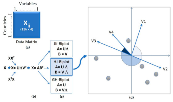
Figure 1.
(a) Structure of the data matrix; (b) phases of the biplot process; (c) types of biplot; (d) representation of individuals and variables.
The relationships between environmental performance indicators, electronic government and corruption perception measures are described by the angles between the vectors; acute angles are associated with a positive correlation. To classify the countries by their indicators of environmental performance, e-government, e-participation and corruption index, that is, by the orthogonal projections of the points (countries) on the vectors (variables), we can order the different countries in relation to each variable.
This method has been applied by Carrasco et al. [32] in hydrology; Cubilla-Montilla et al. [33], Amor-Esteban et al. [34] and García-Sánchez et al. [35] in the context of corporate social responsibility; Castellanos-Martín et al. [36] in breast cancer research; Gallego-Alvarez et al. [37] and Tejedor-Flores [38] to analyse sustainability; Nieto-Librero et al. [39] in geochemical studies; Hernández et al. [40] to study bioactive compounds in agriculture; Mendes et al. [30] in environmental science; García-Talegón [41], in geology, and; Orfao et al [42] in immunology.
2.3. Methodology II: STATIS Method
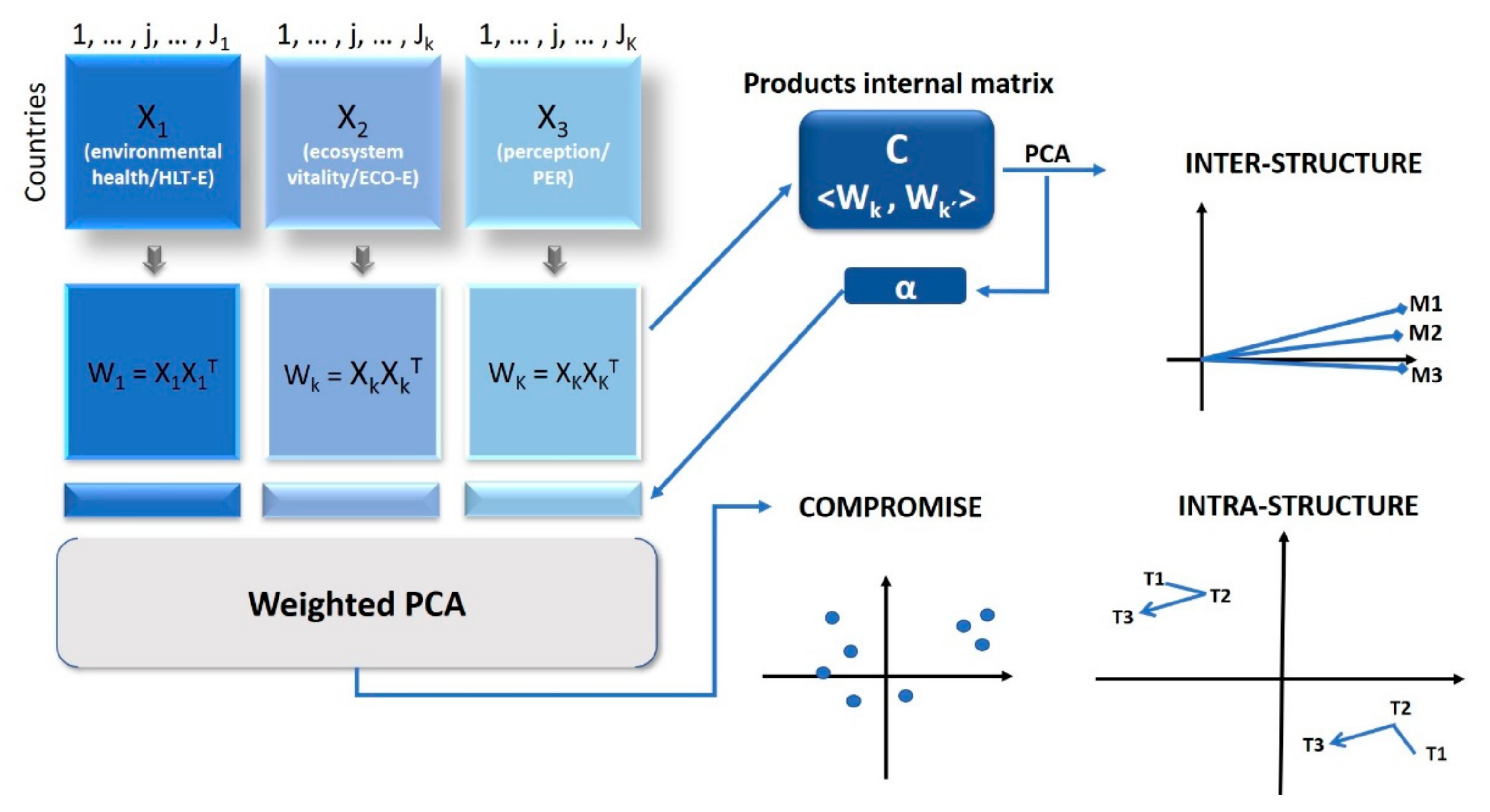
The STATIS method, “structuration des tableaux à trois indices de la statistique” [43], is essentially a generalisation of the principal component analysis (PCA), whose objective is to analyse several sets of variables within a single set of observations in what is called multiple set data. It is a method that allows the exploration of the structure of several data tables. It consists of reducing the dimensionality of the data using a similarity measure based on Euclidean distances between point configurations. The variables may be different in each of the tables.
The STATIS method starts with K tables, with X1, …, XK, k data matrices with J1, …, JK quantitative variables, respectively, observed in the same group of n individuals.
Next, the scalar product between matrices Wk and Wk′ is calculated. To this purpose, a correlation coefficient between matrices is defined; in this case, the vector correlation coefficient RV [44].
The data are arranged in three tables; the first table corresponds to the information of n individuals (countries) measured on p variables (environmental health/HLT-E); the second table has information on the same n individuals measured on q variables (ecosystem vitality/ECO-E), and the third table corresponds to information on the same n individuals measured on r variables (perception/PER). The STATIS method is based on the development of the following steps (see Figure 2):
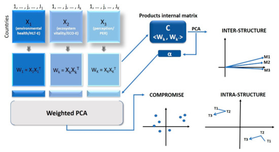
Figure 2.
Figure 2. STATIS scheme: structure of the matrices and phases of the STATIS process.
- Inter-structure analysis: its objective is to make a global comparison of data matrices. A matrix of similarities between individuals (countries) is generated for each matrix, which describes the relationship between matrices.
- Compromise matrix: summarises the matrices into one that is the weighted average of all of them. This matrix synthesises the information of each one of the 116 countries in the variables for the three matrices, ‘filtering the noise’ and representing the statistically significant information.
- Intra-structure analysis: a representation of the countries and variables, which allow exploring the differences or similarities that exist between the data matrices, to define the average position of the countries in the different matrices.
The first works in the framework of this methodology were those carried out by L’Hermier des Plantes and Thiébaut [45] and Lavit [46]. Subsequently, related techniques have been developed such as X-STATIS or Triadic Partial Analysis (PTA) [47], DISTATIS [48] and COVSTATIS [49], all of which take into account data from departure. On the other hand, STATICO (STATIS and COINERTIA) [50,51]; and COSTATIS (COINERTIA AND STATIS) [49] work with pairs of tables in different situations or times. Power-STATIS [52] assigns weights when creating the consensus matrix; whilst t+1 STATIS [53], STATIS-4 [54] and CANOSTATIS [55] take into account external information. The latest contributions have been INTER-STATIS [56] for interval data and CLUSTATIS [57] to group datasets measured in the same individuals.
These methods have been applied in different fields; we can mention the recent works of Fu et al. [58] in data on the user interfaces of mobile shopping applications; Feki-Sahnoun et al. [59] evaluated the biogeography of phytoplankton; Rundle et al. [60] applied it in neurosciences; Amor-Esteban, Galindo-Villardón and García-Sánchez [34] evaluated corporate social responsibility; Marcondes Filho, Fogliatto and Oliveira [61] and Ramos-Barberán et al. [62] proposed control charts based on the STATIS method; Caballero-Julia, Galindo-Villardón and García [63] applied the method to textual data; Bono and Giacomarra [64] measured the performance of technical efficiency in the photovoltaics sector.
The HJ-biplot and STATIS analysis, as well as in the graphs, were performed using the software Multbiplot [65].
3. Results
3.1. HJ-biplot Analysis.
The first part of our analysis is the application of the HJ-biplot method; the objective is to analyse whether there is an association between global corruption indexes (CPI), e-participation (EPI-P), e-government (E-GOV) and environmental performance (EPI-E).
We denote with X the matrix with dimensions n (country), J (variables), where n = 116, number of rows, and J, the number of columns or variables, which in this case are the four global indices; therefore, we have a matrix (116 × 4).
The first axis explains 81.6% of the variability; we will use the 1-2 factorial plane that explains 92.4% of the total variability since it is enough to explore the main characteristics of the data (see Figure 3).
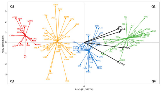
Figure 3.
HJ-biplot representation: the position of all countries in relation to the indices. Mauritius, Georgia, Panama, Rwanda, Dominican Republic and Morocco.
In terms of the indicators, the groups by e-government level are placed on the graph by configuring a gradient from left to right in order: low (red), medium-low (yellow), medium-high (blue) and high e-government (green). This means that the main reason for the separation of the countries is the level of e-government since it is the characteristic that is represented in the abscissa axis, which is the axis that retains the greatest variation because it is associated with the greater eigenvalue. It should be noted that most countries achieved a good quality of representation at this level, although this was somewhat lower for Iran, Venezuela, Sri Lanka, Kuwait, Argentina, and Albania.
The four indicators correlate with each other; however, we observe that there is a closer correlation between the corruption perception indicator (CPI) and the environmental performance indicator (EPI-E); the lower the level of corruption, the higher the index of environmental performance (EPI-E). On the other hand, e-government (E-GOV) and e-participation (EPI-P) indices demonstrate an association, which is expected, since they measure the levels of e-government and e-participation.
The countries located in the first quadrant (Q1) have the lowest rates of corruption (CPI) and the highest rates of environmental performance (EPI-E), meaning that their priorities are to improve environmental performance and reduce corruption. Among the countries that make up this group, we can mention Switzerland, Denmark, Iceland, Austria, Belgium and Sweden, among others, which possess a high economic income. In the fourth quadrant (Q4) are the countries that give higher priority to electronic government (E-GOV) and citizen electronic participation (EPI-P), which have high economic income (for example, Korea, USA, Spain and Japan). Between the second (Q2) and third (Q3) quadrants, there are the countries with the lowest rates, among which we can mention Central African Republic, Afghanistan, Haiti, Egypt, Nicaragua and India, possessing low and medium–low economic income.
3.2. STATIS Analysis
The second part of our analysis is the implementation of the STATIS method, which will allow us to analyse the importance of the dimensions, in addition to studying the similarities and differences between the indicators of each dimension. Thus, we denote with Xk data matrices with I equal to 116 rows (countries) and Jk variables, where K (studies/dimensions) is the number of tables or matrices. Therefore, we obtain three matrices (I × Jk): the first matrix has three indicators of the HLT-E; the second has seven indicators of the ECO-E, and the third with has three indicators of the perception dimension.
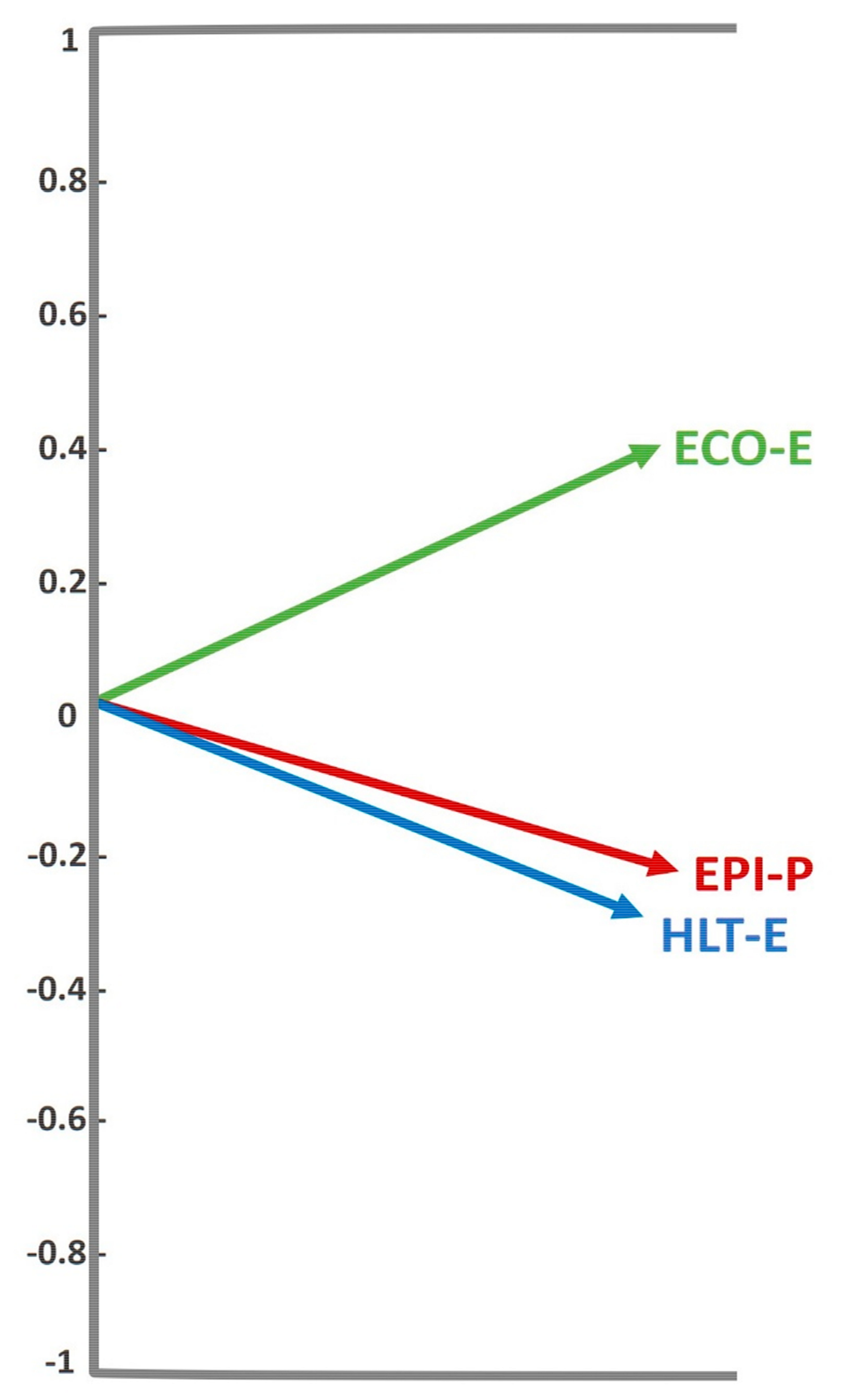
As a first step, we will obtain the inter-structure, consisting of the comparison of the structures of the three matrices of the study. The vector correlation matrix is calculated, which allows us to observe the relationship between the matrices. When analysing the vector correlation coefficients (RV) and the distances between the matrices, two similar dimensions are observed, HLT-E and perception (PER) with an RV coefficient of 0.687, while the ECO-E is slightly different. The Euclidean representation in Figure 4 identifies the proximity between the matrices. Factorial plane 1-2 explains 89.6% of the total information.

Figure 4.
Inter-structure of the three matrices.
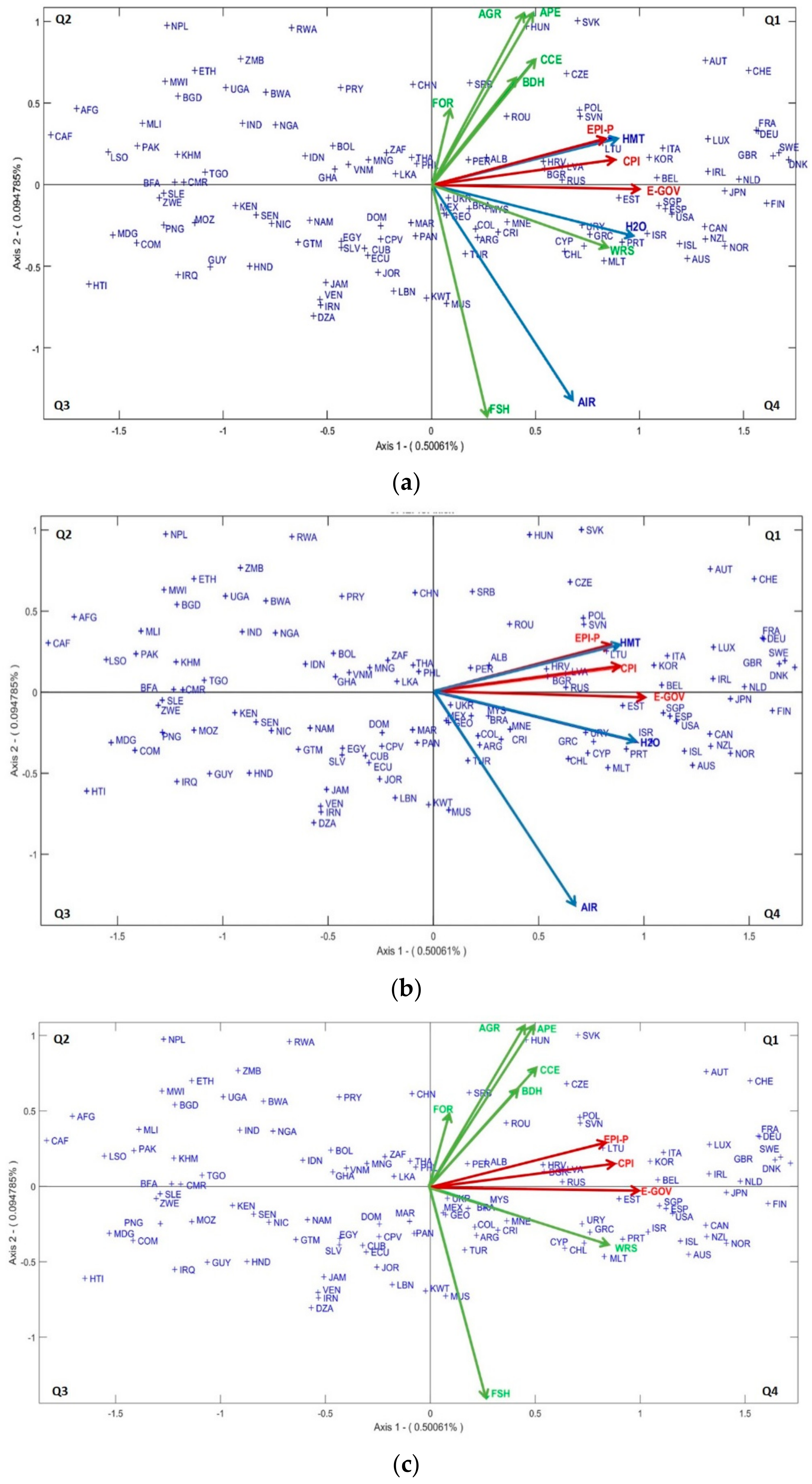
In the second step, a matrix is constructed that summarises and synthesises the common structure of all the original matrices: the compromise matrix. With this matrix, the behaviour of countries in the three matrices as a whole is compared and evaluated. The information collected by the first two axes is 59.5%, enough for our analysis. The first axis carries most of the information with 50.1%. Indicators and countries on compromise are represented in Figure 5a.
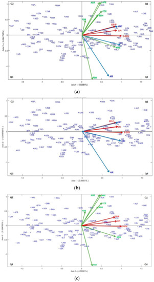
Figure 5.
STATIS compromise subspace: (a) the position of 116 countries with respect to the 13 indicators; (b) indicators of the environmental health (HLT-E) and e-participation (EPI-E) matrices; (c) indicators of the ecosystem vitality (ECO-E) and perception (PER) matrices.
The indicators are represented by the vectors; the green ones correspond to the vitality dimension of the ecosystem (ECO-E), the red ones to the perception dimension (PER) and the blue ones to the HLT-E. All are located in quadrants 1 (Q1) and 4 (Q4) (right half-plane). The countries that are located in this semi-plane have the highest indicators across all dimensions. Strong correlations are observed between the variables of the HLT-E dimension to the PER dimension, except two indicators: air quality (AIR) and fisheries management (FSH). The strongest relationship is between e-participation (EPI-P) and lead exposure (HMT). We can form three dimensions: the first being the relationship with “ecological issues”; the second with “transparent government”; the third we will call “air and fishing”.
Regarding Environmental Health (HLT-E), all indicators are located between quadrants 1 (Q1) and 4 (Q4) (right half-plane). The countries that position themselves in this semi-plane give greater relevance to lowering levels of heavy metal pollution (HMT), water care and sanitation (H2O) and improving air quality (AIR). On the other hand, they show a high value to e-government (E-GOV), e-participation (EPI-P) and very low values the corruption index (CPI) (see Figure 5b).
In Figure 5c, the ECO-E scenario is shown; the indicators are located in the right half-plane. The countries that are located in quadrant 1 (Q1) give greater importance to improving the indicators we call “ecological issues”; these are forests (FOR), agriculture (AGR), climate and energy (CCE) and air pollution (APE), while those in quadrant IV place greater importance on fisheries management (FISH) and water sources (WRS).
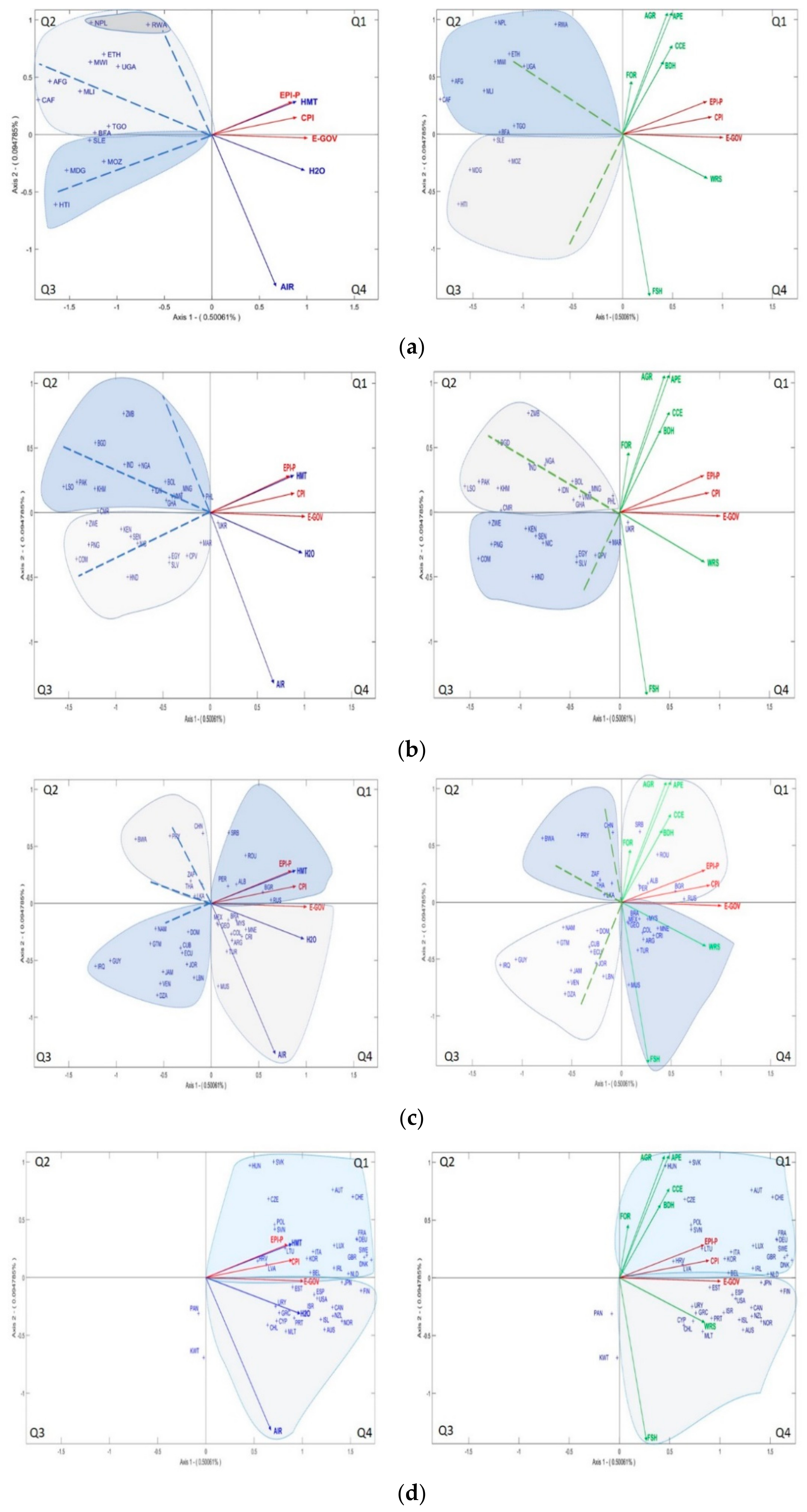
To evaluate the effects of the level of income on environmental performance, we use the level income of the countries. In this way, we visualise the behaviour patterns of the countries. For this reason, and to obtain a better understanding, we project the countries in the commitment subspace, dividing them into the four levels of income (see Figure 6).

Figure 6.
Factorial plane 1–2 of the compromise subspace, divided into the 4 levels of economic income: (a) low level; (b) medium–low level; (c) medium–high level; (d) high level.
Countries with low economic income show very low values to environmental performance and on perception indices; located at the left end of quadrants 2 (Q2) and 3 (Q3) (left half-plane), they have the lowest values in all their indicators, in relation to the other countries (see Figure 6a). These are notably different with respect to those of the right half-plane. Most of these countries are located in quadrant 2 (Q2), show low levels of air quality (AIR) and low levels of drinking water and sanitation (H2O), as well as low levels of wastewater treatment (WRS). Countries that are located in quadrant 3 (Q3) are characterised as having high levels of exposure to lead (HMT) and in general, very low levels of all indicators of ECO-E. This group includes Nepal (NPL) and Rwanda (RWA) with high levels of air pollution, Haiti (HTI) with high levels of lead exposure, and the Central African Republic (CAF) together with Afghanistan (AFG), both with low levels of drinking water and sanitation. On the other hand, they have low levels of e-participation and e-government and very high levels of corruption.
Figure 6b shows the middle-low income countries, which follow a pattern similar to the previous group, albeit with slightly higher indicators. They have low values in all their indicators. They are distributed in quadrants 2 (Q2) and 3 (Q3) and show deficiencies in the indicators of environmental health (HLT-E) and ecosystem vitality (ECO-E).
The countries with medium–high economic income show better indicators and are distributed in across four quadrants (see Figure 6c). Those located in quadrants 2 (Q2) and 3 (Q3) have lower indicators than those located in quadrants 1 (Q1) and 4 (Q4). Within this group, those located in quadrant 2 (Q2) have deficiencies in air quality (AIR), drinking water and sanitation (H2O) and in wastewater treatment (WRS); however, they are better positioned than the two previous groups. On the opposite end (Q4), countries with better values are located in these same indicators. On the other hand, the countries in this group, which are located in quadrant 1 (Q1), they have higher values in all their indicators, especially with regard to the indicators of ecosystem vitality (ECO-E) and e-participation. The countries with slightly lower values are positioned in quadrant 3 (Q3).
Finally, Figure 6d shows the high-income countries, which are characterised by leading all indicators. However, they are distributed in quadrants 1 (Q1) and 4 (Q4), indicating that this group places a higher priority on the indicators of ECO-E and others than environmental health (HLT-E). Thus we have a small group of countries leading in decreasing SO2 emissions (APE), sustainable nitrogen management (AGR), climate and energy (CCE) and biodiversity and habitat (BDH); the countries that are located near axis 1 lead as regards e-government (EGOV), e-participation (EPI-P) and low levels of corruption (CPI); while those located in the fourth quadrant focus on better quality drinking water and adequate sanitation (H2O) and on wastewater treatment (WRS).
Countries with the best environmental performance and transparent governments are Switzerland (CHE), France (FRA), Germany (DEU), Sweden (SWE), Denmark (DNK) and Finland (FIN). On the other hand, countries with lower levels of environmental performance and higher levels of corruption are Central African Republic (CAF), Afghanistan (AFG), Haiti (HTI) and Madagascar (MDG).
4. Discussion
It has been shown that the combination of the HJ-biplot and STATIS methods allows us to easily observe the environmental performance index (EPI-E) and the indicators of e-government, e-participation and corruption in a single structure.
The application of the HJ-biplot method facilitated the representation of the 116 countries and the four global indicators in a graph, plotting the countries and indicators of the data matrix as points in a small vector space. The STATIS method showed the underlying structures of the data concerning relations between the different indicators and how they comprehensively explained the similarities and differences between countries.
E-participation has increased in recent decades; this is due to the popularisation of social networks; however, in our findings, we observe that e-participation is very low in low and middle-income countries. As noted by Bicking et al. [66] and Koussouris et al. [67], there are many challenges to converting existing users of e-participation platforms into more active users, in addition to encouraging those who still do not use them. The lagging development of technological infrastructures diminishes the e-participation. Improvement in this factor will help to enrich the quality of the debate, legitimising decision-making, particularly in environmental matters.
From the point of view of government institutions, these are thought to be inadequate to meet the challenges related to environmental performance [68]. Some researchers such as Beierle and Cayford [69] and Newig and Fritsch [70] point out that citizen participation has a significant influence on environmental governance and sustainability. In this sense, our findings show that those countries with very high e-government and e-participation levels show the best indicators of environmental performance, especially in those related to environmental health.
Alió and Gallego [71], on the one hand, and Royo and Yetano [72], on the other, point out that in matters of sustainability, citizen participation plays a critical role. As Royo, Yetano and Acerete [68] identified, the global effort for environmental protection goes hand-in-hand with citizens well-informed of environmental policies and initiatives. Our results are along this vein; as we have discovered, there is a correlation between high levels of e-participation and environmental performance indicators.
Another of our results shows that countries with low levels of income have low levels of environmental performance and those countries with high levels of income also have high levels of environmental performance.
The results obtained allow us to affirm that there is a certain articulation between the e-government, e-participation and the environmental performance indices; this suggests that the issues of environmental performance are applied by governments that have a style of public administration more inclined towards citizen participation, which supports the evidence revealed by García-Sánchez, Rodríguez-Domínguez and Gallego-Álvarez [73].
5. Conclusions
The results of the HJ-biplot show us that there is a closer correlation between the CPI and the EPI-E, which indicates that the lower the level of corruption, the higher the EPI-E. Countries are grouped according to their e-government level.
A common behaviour is presented between environmental health dimension (HLT-E) and perception dimension (PER). Those countries with high levels of e-participation (EPI-P) also show lower levels of corruption (CPI).
Concerning income level, countries with low and medium–low economic income are characterised by lagging in all environmental performance indicators, as well as reflecting very low levels of e-government (E-GOV) and e-participation (EPI-P) and very high levels of corruption (CPI). While those with medium–high incomes reflect better indicators, a large number of these countries struggle to keep up. We could say that they are in a transition to better states of environmental performance. As for high-income countries, all of them reflect high levels of environmental performance, citizen participation and the reduction of corruption.
Countries that exhibit greater e-participation, lower levels of corruption and better level income are more likely to follow policies and programmes aimed at achieving better environmental performance. Our results suggest that e-participation is important in improving environmental performance.
In future studies, we recommend placing further emphasis on the real impact of e-participation in national environmental policies and programmes, expanding the qualitative analysis of specific actions in national organisations, and changes in government actions resulting from the use of e-participation.
Author Contributions
Conceptualization, C.C.R.-M., P.G.-V. and I.M.G.-S.; Data curation, C.C.R.-M.; Formal analysis, C.C.R.-M., P.V.-G. and I.M.G.-S.; Funding acquisition, C.C.R.-M.; Methodology, P.V.-G. and P.G.-V.; Project administration, I.M.G.-S.; Supervision, P.G.-V. and I.M.G.-S.; Writing—original draft, C.C.R.M.; Writing—review & editing, C.C.R.-M., P.V.-G., P.G.-V. and I.M.G.-S.
Funding
This research was funded by the National Secretary of Science and Technology of Panama (SENACYT), doctoral scholarship programme.
Acknowledgments
The author thanks Mitzi I. Cubilla M., PhD, for her support in editing this document; and to the anonymous reviewers for their comments, which helped improve the document.
Conflicts of Interest
The authors declare no conflict of interest in the results.
Appendix A

Table A1.
Classification of countries by level income.
Table A1.
Classification of countries by level income.
| Low Income $1035 or less | Low–Middle Income $1036–4085 | High–Middle Income $4086–12,615 | High Income $12,616 or more |
|---|---|---|---|
| Afghanistan (AFG) | Bangladesh (BGD) | Albania (ALB) | Australia (AUS) |
| Burkina Faso (BFA) | Bolivia (BOL) | Algeria (DZA) | Austria (AUT) |
| Central African Republic (CAF) | Cameroon (CMR) | Argentina (ARG) | Bélgium (BEL) |
| Ethiopia (ETH) | Comoros (COM) | Botswana (BWA) | Canada (CAN) |
| Haiti (HTI) | Cabo verde (CPV) | Brazil (BRA) | Chile (CHL) |
| Madagascar (MDG) | Cambodia (KHM) | Bulgaria (BGR) | Croatia (HRV) |
| Malawi (MWI) | Egypt, Arab Rep. (EGY) | China (CHN) | Cyprus (CYP) |
| Mali (MLI) | El Salvador (SLV) | Colombia (COL) | Czech Republic (CZE) |
| Mozambique (MOZ) | Ghana (GHA) | Costa Rica (CRI) | Denmark (DNK) |
| Nepal (NPL) | Honduras (HND) | Cuba (CUB) | Estonia (EST) |
| Rwanda (RWA) | India (IND) | Dominican Republic (DOM) | Finland (FIN) |
| Sierra Leone (SLE) | Indonesia (IDN) | Ecuador (ECU) | France (FRA) |
| Togo (TGO) | Kenya (KEN) | Georgia (GEO) | Germany (DEU) |
| Uganda (UGA) | Lesotho (LSO) | Guatemala (GTM) | Greece (GRC) |
| Mongolia (MNG) | Guyana (GUY) | Hungary (HUN) | |
| Morocco (MAR) | Irán, Islamic Rep. (IRN) | Iceland (ISL) | |
| Nicaragua (NIC) | Iraq (IRQ) | Ireland (IRL) | |
| Nigeria (NGA) | Jamaica (JAM) | Israel (ISR) | |
| Pakistan (PAK) | Jordan (JOR) | Italy (ITA) | |
| Papúa Nueva Guinea (PNG) | Lebanon (LBN) | Japan (JPN) | |
| Philippines(PHL) | Malaysia (MYS) | Korea, Rep. (KOR) | |
| Senegal (SEN) | Mauritius (MUS) | Kuwait (KWT) | |
| Ukraine (UKR) | Mexico (MEX) | Latvia (LVA) | |
| Vietnam (VNM) | Montenegro (MNE) | Lithuania (LTU) | |
| Zambia (ZMB) | Namibia (NAM) | Luxembourg (LUX) | |
| Zimbabwe (ZWE) | Paraguay (PRY) | Malta (MLT) | |
| Perú (PER) | Netherlands (NLD) | ||
| Romania (ROU) | New Zealand (NZL) | ||
| Russian Federation (RUS) | Norway (NOR) | ||
| Serbia (SRB) | Panama (PAN) | ||
| Sri Lanka (LKA) | Poland (POL) | ||
| South Africa (ZAF) | Portugal (PRT) | ||
| Thailand (THA) | Singapore (SGP) | ||
| Turkey (TUR) | Slovak Republic (SVK) | ||
| Venezuela, RB (VEN) | Slovenia (SVN) | ||
| Spain (ESP) | |||
| Sweden (SWE) | |||
| Switzerland (CHE) | |||
| United Kingdom (GBR) | |||
| United States (USA) | |||
| Uruguay (URY) |
Note: Bold indicates a change of classification. Source: World Bank, © The World Bank Group [74].
References
- Wang, Z.; Zhang, B.; Wang, B. The moderating role of corruption between economic growth and CO2 emissions: Evidence from BRICS economies. Energy 2018, 148, 506–513. [Google Scholar] [CrossRef]
- Burakov, D.; Bass, A. Institutional determinants of environmental pollution in Russia: A non-linear ARDL approach. Entrep. Sustain. Issues 2019, 7, 510–524. [Google Scholar] [CrossRef]
- Aniscenko, Z.; Robalino-López, A.; Rodríguez, T.E.; Pérez, B.E. Regional cooperation in dealing with environmental protection. E-government and sustainable development in Andean countries. In Proceedings of the 11th International Scientific and Practical Conference, Rezekne, Latvia, 15–17 June 2017. [Google Scholar]
- Flores, O.M. Gestión ambiental urbana y desarrollo sustentable. Consideraciones desde un enfoque social sobre nuestro hábitat urbano. Rev. Electrón. Ambient. Total 2009, 1, 1–8. [Google Scholar]
- Di Vaio, A.; Varriale, L. Management innovation for environmental sustainability in seaports: Managerial accounting instruments and training for competitive green ports beyond the regulations. Sustainability 2018, 10, 783. [Google Scholar] [CrossRef]
- Wendling, Z.A.; Emerson, J.W.; Esty, D.C.; Levy, M.A.; de Sherbinin, A. Environmental Performance Index; Yale Center for Environmental Law & Policy: New Haven, CT, USA, 2018. [Google Scholar]
- Justice, J.B.; Melitski, J.; Smith, D.L. E-government as an instrument of fiscal accountability and responsiveness: Do the best practitioners employ the best practices? Am. Rev. Public Adm. 2006, 36, 301–322. [Google Scholar] [CrossRef]
- Torres, L.; Pina, V.; Acerete, B. E-government developments on delivering public services among EU cities. Gov. Inf. Q. 2005, 22, 217–238. [Google Scholar] [CrossRef]
- Siau, K.; Long, Y. Using social development lenses to understand e-government development. J. Glob. Inf. Manag. 2006, 14, 47–62. [Google Scholar] [CrossRef]
- Tolbert, C.J.; Mossberger, K. The effects of e-government on trust and confidence in government. Public Adm. Rev. 2006, 66, 354–369. [Google Scholar] [CrossRef]
- Navarro-Galera, A.; Alcaraz-Quiles, F.J.; Ortiz-Rodriguez, D. Enhancing sustainability transparency in local governments—An empirical research in Europe. Sustainability 2018, 10, 2161. [Google Scholar] [CrossRef]
- Macintosh, A.; Whyte, A. Towards an evaluation framework for eParticipation. Transform. Gov. People Process Policy 2008, 2, 16–30. [Google Scholar] [CrossRef]
- Serov, I.; Leitner, M. An experimental approach to reputation in e-participation. In Proceedings of the 2016 International Conference on Software Security and Assurance (ICSSA), St. Polten, Austria, 24–25 August 2016; pp. 37–42. [Google Scholar]
- Armah, F.A.; Yawson, D.O.; Pappoe, A.N.M.; Afrifa, E.K.A. Participation and sustainable management of coastal lagoon ecosystems: The case of the Fosu Lagoon in Ghana. Sustainability 2010, 2, 383–399. [Google Scholar] [CrossRef]
- United Nations. E-Government Survey 2012: E-Government for the People; United Nations: New York, NY, USA, 2012. [Google Scholar]
- Voß, J.-P.; Newig, J.; Kastens, B.; Monstadt, J.; Nölting, B. Steering for sustainable development: A typology of problems and strategies with respect to ambivalence, uncertainty and distributed power. J. Environ. Policy Plan. 2007, 9, 193–212. [Google Scholar] [CrossRef]
- Renn, O.; Schweizer, P.-J. Inclusive risk governance: Concepts and application to environmental policy making. Environ. Policy Gov. 2009, 19, 174–185. [Google Scholar] [CrossRef]
- Wellalage, N.H.; Locke, S.; Samujh, H. Corruption, gender and credit constraints: Evidence from South Asian SMEs. J. Bus. Ethics 2019, 159, 267–280. [Google Scholar] [CrossRef]
- Masud, M.A.K.; Bae, S.M.; Manzanares, J.; Kim, J.D. Board directors’ expertise and corporate corruption disclosure: The moderating role of political connections. Sustainability 2019, 11, 4491. [Google Scholar] [CrossRef]
- Windsor, D. International business, corruption, and bribery. In Advances in Sustainability and Environmental Justice; Emerald Group Publishing Limited: Bingley, UK, 2013; pp. 65–95. ISBN 9781781906255. [Google Scholar]
- Kim, E.; Ha, Y.; Kim, S. Public debt, corruption and sustainable economic growth. Sustainability 2017, 9, 433. [Google Scholar] [CrossRef]
- Previtali, P.; Cerchiello, P. The prevention of corruption as an unavoidable way to ensure healthcare system sustainability. Sustainability 2018, 10, 3071. [Google Scholar] [CrossRef]
- Lisciandra, M.; Migliardo, C. An empirical study of the impact of corruption on environmental performance: Evidence from panel data. Environ. Resour. Econ. 2017, 68, 297–318. [Google Scholar] [CrossRef]
- Yale Center for Environmental Law and Policy—YCELP—Yale University; Yale Data-Driven Environmental Solutions Group—Yale University; Center for International Earth Science Information Network—CIESIN—Columbia University; World Economic Forum—WEF. 2018 Environmental Performance Index (EPI). Available online: https://sedac.ciesin.columbia.edu/data/set/epi-environmental-performance-index-2018 (accessed on 1 May 2018).
- United Nations (UN). E-Government Knowledge Database (UNeGovDD). Available online: https://publicadministration.un.org/egovkb/en-us/ (accessed on 10 February 2019).
- TI-Transparency International Corruption Perception Index. 2018. Available online: https://www.transparency.org/cpi2018 (accessed on 10 February 2019).
- World Bank. World Bank’s Indicators Database. 2018. Available online: https://datos.bancomundial.org/indicador (accessed on 4 April 2018).
- Galindo-Villardón, M.P. An alternative for simultaneous representation: HJ-biplot. Questiió 1986, 10, 12–23. [Google Scholar]
- Gabriel, K.R. The biplot graphic display of matrices with application to principal component analysis. Biometrika 1971, 58, 453–467. [Google Scholar] [CrossRef]
- Mendes, S.; Fernández-Gómez, M.; Galindo, M.; Morgado, F.; Maranhão, P.; Azeiteiro, U.; Bacelar-Nicolau, P. The study of bacterioplankton dynamics in the Berlengas Archipelago (West coast of Portugal) by applying the HJ-biplot method. Arquipel. Life Mar. Sci. 2009, 26, 25–35. [Google Scholar]
- Eckart, C.; Young, G. The approximation of one matrix by another of lower rank. Psychometrika 1936, 1, 211–218. [Google Scholar] [CrossRef]
- Carrasco, G.; Molina, J.-L.; Patino-Alonso, M.-C.; Castillo, M.D.C.; Vicente-Galindo, M.-P.; Galindo-Villardón, M.-P. Water quality evaluation through a multivariate statistical HJ-biplot approach. J. Hydrol. 2019, 577, 123993. [Google Scholar] [CrossRef]
- Cubilla-Montilla, M.; Nieto-Librero, A.-B.; Galindo-Villardón, M.P.; Vicente Galindo, M.P.; Garcia-Sanchez, I.-M. Are cultural values sufficient to improve stakeholder engagement human and labour rights issues? Corp. Soc. Responsib. Environ. Manag. 2019, 26, 938–955. [Google Scholar] [CrossRef]
- Amor-Esteban, V.; Galindo-Villardón, M.-P.; García-Sánchez, I.-M. Industry mimetic isomorphism and sustainable development based on the X-STATIS and HJ-biplot methods. Environ. Sci. Pollut. Res. 2018, 25, 26192–26208. [Google Scholar] [CrossRef]
- García-Sánchez, I.-M.; Frías-Aceituno, J.-V.; Rodríguez-Domínguez, L. Determinants of corporate social disclosure in Spanish local governments. J. Clean. Prod. 2013, 39, 60–72. [Google Scholar] [CrossRef]
- Castellanos-Martín, A.; Castillo-Lluva, S.; Sáez-Freire, M.D.M.; Blanco-Gómez, A.; Hontecillas-Prieto, L.; Patino-Alonso, C.; Galindo-Villardon, P.; del Villar, L.P.; Martín-Seisdedos, C.; Isidoro-Garcia, M.; et al. Unraveling heterogeneous susceptibility and the evolution of breast cancer using a systems biology approach. Genome Biol. 2015, 16, 40. [Google Scholar] [CrossRef]
- Gallego-Álvarez, I.; Galindo-Villardón, M.P.; Rodríguez-Rosa, M. Analysis of the sustainable society index worldwide: A study from the biplot perspective. Soc. Indic. Res. 2015, 120, 29–65. [Google Scholar] [CrossRef]
- Tejedor-Flores, N.; Vicente-Galindo, P.; Galindo-Villardón, P. Sustainability multivariate analysis of the energy consumption of ecuador using MuSIASEM and BIPLOT approach. Sustainability 2017, 9, 984. [Google Scholar] [CrossRef]
- Nieto-Librero, A.B.; Sierra, C.; Vicente-Galindo, M.P.; Ruíz-Barzola, O.; Galindo-Villardón, M.P. Clustering Disjoint HJ-biplot: A new tool for identifying pollution patterns in geochemical studies. Chemosphere 2017, 176, 389–396. [Google Scholar] [CrossRef]
- Hernández, M.; Espinosa, F.; Galindo, P. Tomato fruit quality as influenced by the interactions between agricultural techniques and harvesting period. J. Plant Nutr. Soil Sci. 2014, 177, 443–448. [Google Scholar] [CrossRef]
- Garcia-Talegon, J.; Vicente, M.A.; Molina-Ballesteros, E.; Vicente-Tavera, S. Determination of the origin and evolution of building stones as a function of their chemical composition using the inertia criterion based on an HJ-biplot. Chem. Geol. 1999, 153, 37–51. [Google Scholar] [CrossRef]
- Orfao, A.; Gonzalez, M.; san Miguel, J.F.; Cañizo, M.C.; Galindo, P.; Caballero, M.D.; Jimenez, R.; Borrasca, A.L. Clinical and immunological findings in large B-cell chronic lymphocytic leukemia. Clin. Immunol. Immunopathol. 1988, 46, 177–185. [Google Scholar] [CrossRef]
- Des Plantes, H.L. Structuration des Tableaux à Trois Indices de la Statistique. Ph.D. Thesis, Université de Montpellier II, Montpellier, France, 1976. [Google Scholar]
- Escoufier, Y. Le traitement des variables vectorielles. Biometrics 1973, 29, 751–760. [Google Scholar] [CrossRef]
- Des Plantes, H.L.; Thiébaut, B. Evue de statistique appliquée. Rev. Stat. Appl. 1977, 25, 57–81. [Google Scholar]
- Lavit, C. Analyse Conjointe de Tableaux Quantitatifs; Masson: Paris, France, 1988; ISBN 2225814783. [Google Scholar]
- Jaffrenou, P.A. Sur L’Analyse des Familles Finies des Variables Vectorielles: Bases Algébrique et Application à la Description Statistique. Ph.D. Thesis, l’Université de Sainte-Etiene, Saint-Étienne, France, 1978. [Google Scholar]
- Abdi, H.; Valentin, D.; Chollet, S.; Chrea, C. Analyzing assessors and products in sorting tasks: DISTATIS, theory and applications. Food Qual. Prefer. 2007, 18, 627–640. [Google Scholar] [CrossRef]
- Thioulouse, J. Simultaneous analysis of a sequence of paired ecological tables: A comparison of several methods. Ann. Appl. Stat. 2011, 5, 2300–2325. [Google Scholar] [CrossRef]
- Simier, M.; Blanc, L.; Pellegrin, F.; Nandris, D. Approche simultanee de k couples de tableaux: Application à l´étude des relations pathologie végétale-environnement. Rev. Stat. Appl. 1999, 47, 31–46. [Google Scholar]
- Thioulouse, J.; Simier, M.; Chessel, D. Simultaneous analysis of a sequence of paired ecological tables. Ecology 2004, 85, 272–283. [Google Scholar] [CrossRef]
- Bénasséni, J.; Bennani-Dosse, M. Analyzing multiset data by the Power STATIS-ACT method. Adv. Data Anal. Classif. 2012, 6, 49–65. [Google Scholar] [CrossRef]
- Sauzay, L.; Hanafi, M.; Qannari, E.M.; Schlich, P. Analyse de K + 1 tabléaux a l’aide de la méthode STATIS: Application en evaluation sensorielle. In 9ième Journées Européennes Agro-industrie et Méthodes Statistiques; Faculté de Pharmacie: Montpellier, France, 2006; pp. 1–23. [Google Scholar]
- Sabatier, R.; Vivien, M. A new linear method for analyzing four-way multiblocks tables: STATIS-4. J. Chemom. 2008, 22, 399–407. [Google Scholar] [CrossRef]
- Vallejo-Arboleda, A.; Vicente-Villardón, J.L.; Galindo-Villardón, M.P.P. Canonical STATIS: Biplot analysis of multi-table group structured data based on STATIS-ACT methodology. Comput. Stat. Data Anal. 2007, 51, 4193–4205. [Google Scholar] [CrossRef]
- Corrales, D.; Rodríguez, O. Interstatis: El método statis para datos de tipo intervalo. Rev. Mat. Teor. Apl. 2014. [Google Scholar] [CrossRef]
- Llobell, F.; Cariou, V.; Vigneau, E.; Labenne, A.; Qannari, E.M. Analysis and clustering of multiblock datasets by means of the STATIS and CLUSTATIS methods. Application to sensometrics. Food Qual. Prefer. 2018, 79, 103520. [Google Scholar] [CrossRef]
- Fu, Y.; Jiang, H.; Zhang, D.; Zhang, X. Comparison of perceptual differences between users and designers in mobile shopping app interface design: Implications for evaluation practice. IEEE Access 2019, 7, 23459–23470. [Google Scholar] [CrossRef]
- Feki-Sahnoun, W.; Hamza, A.; Béjaoui, B.; Mahfoudi, M.; Rebai, A.; Hassen, M.B. Multi-table approach to assess the biogeography of phytoplankton: Ecological and management implications. Hydrobiologia 2018, 815, 229–251. [Google Scholar] [CrossRef]
- Rundle, M.M.; Coch, D.; Connolly, A.C.; Granger, R.H. Dissociating frequency and animacy effects in visual word processing: An fMRI study. Brain Lang. 2018, 183, 54–63. [Google Scholar] [CrossRef]
- Filho, D.M.; Fogliatto, F.S.; de Oliveira, L.P.L. Monitoring nonlinear batch process using statis-based method. In Applied Mechanics and Materials; Trans Tech Publications: Stafa-Zurich, Switzerland, 2014. [Google Scholar]
- Ramos-Barberán, M.; Hinojosa-Ramos, M.V.; Ascencio-Moreno, J.; Vera, F.; Ruiz-Barzola, O.; Galindo-Villardón, M.P. Batch process control and monitoring: A Dual STATIS and Parallel Coordinates (DS-PC) approach. Prod. Manuf. Res. 2018, 6, 470–493. [Google Scholar] [CrossRef]
- Caballero-Juliá, D.; Galindo-Villardón, M.P.; García, M.-C. JK-Meta-Biplot y STATIS Dual como herramientas de análisis de tablas textuales múltiples. RISTI 2017, 25, 18–33. [Google Scholar] [CrossRef][Green Version]
- Bono, F.; Giacomarra, M. The photovoltaic growth in the European Union requires stronger RES support. J. Policy Model. 2016, 38, 324–339. [Google Scholar] [CrossRef]
- Vicente-Villardón, J.L. MULTBIPLOT: A Package for Multivariate Analysis Using Biplots; Universidad de Salamanca: Salamanca, Spain, 2010. [Google Scholar]
- Bicking, M.; Triantafillou, A.; Henderson, F.; Koussouris, S.; Wimmer, M.A. 2011 IST-Africa conference proceedings. In Proceedings of the IST-Africa 2011 Conference, Gaborone, Botswana, 11–13 May 2011; pp. 1–8. [Google Scholar]
- Koussouris, S.; Charalabidis, Y.; Askounis, D. A review of the European Union eParticipation action pilot projects. Transform. Gov. People Process Policy 2011, 5, 8–19. [Google Scholar] [CrossRef]
- Royo, S.; Yetano, A.; Acerete, B. E-participation and environmental protection: Are local governments really committed? Public Adm. Rev. 2014, 74, 87–98. [Google Scholar] [CrossRef]
- Beierle, T.C.; Cayford, J. Democracy in Practice: Public Participation in Environmental Decisions; Resources for the Future: Washington, DC, USA, 2002; ISBN 9781891853548. [Google Scholar]
- Newig, J.; Fritsch, O. Environmental governance: Participatory, multi-level—And effective? Environ. Policy Gov. 2009, 19, 197–214. [Google Scholar] [CrossRef]
- Alió, M.À.; Gallego, A. Civic entities in environmental local planning. A contribution from a participative research in the metropolitan area of Barcelona. Geojournal 2002, 56, 123–134. [Google Scholar] [CrossRef]
- Royo, S.; Yetano, A. “Crowdsourcing” as a tool for e-participation: Two experiences regarding CO2 emissions at municipal level. Electron. Commer. Res. 2015, 15, 323–348. [Google Scholar] [CrossRef]
- Garciá-Sánchez, I.M.; Rodríguez-Domínguez, L.; Gallego-Álvarez, I. The relationship between political factors and the development of e-participatory government. Inf. Soc. 2011, 27, 233–251. [Google Scholar] [CrossRef]
- World Bank. World Bank Country and Lending Groups. © The World Bank Group. 2019. Available online: https://datahelpdesk.worldbank.org/knowledgebase/articles/906519 (accessed on 12 February 2019).
© 2019 by the authors. Licensee MDPI, Basel, Switzerland. This article is an open access article distributed under the terms and conditions of the Creative Commons Attribution (CC BY) license (http://creativecommons.org/licenses/by/4.0/).


