Numerical Simulation of the Aeroelastic Response of Wind Turbines in Typhoons Based on the Mesoscale WRF Model

Abstract

A new simulation method for the aeroelastic response of wind turbines under typhoons is proposed. The mesoscale Weather Research and Forecasting (WRF) model was used to simulate a typhoon’s average wind speed field. The measured power spectrum and inverse Fourier transform method were coupled to simulate the pulsating wind speed field. Based on the modal method and beam theory, the wind turbine model was constructed, and the GH-BLADED commercial software package was used to calculate the aerodynamic load and aeroelastic response. The proposed method was applied to assess aeroelastic response characteristics of a commercial 6 MW offshore wind turbine under different wind speeds and direction variation patterns for the case study of typhoon Hagupit (2008), with a maximal wind speed of 230 km/h. The simulation results show that the typhoon’s average wind speed field and turbulence characteristics simulated by the proposed method are in good agreement with the measured values: Their difference in the main flow direction is only 1.7%. The scope of the wind turbine blade in the typhoon is significantly larger than under normal wind, while that under normal operation is higher than that under shutdown, even at low wind speeds. In addition, an abrupt change in wind direction has a significant impact on wind turbine response characteristics. Under normal operation, a sharp variation of the wind direction by 90 degrees in 6 s increases the wind turbine (WT) vibration scope by 27.9% in comparison with the case of permanent wind direction. In particular, the maximum deflection of the wind tower tip in the incoming flow direction reaches 28.4 m, which significantly exceeds the design standard safety threshold.

1. Introduction

Offshore wind turbines (WT) enjoy the advantages of vast energy reserves, high wind speeds, low turbulence, and long-term operation hours, which imply their excellent development prospects [1,2]. However, the safety of globally developed offshore wind farms is jeopardized by hurricanes in extratropical conditions and by typhoons in tropical ones [3,4].

Typhoons are mesoscale atmospheric vortex systems with a tremendous energy, which makes them extremely destructive. They differ from ordinary strong winds and hurricanes by their more intensive rotation and their convergent airflows, extreme wind speeds and turbulence intensities, ascending and sinking airflows, sharp changes in the wind direction, etc. [5,6]. Since most high-power offshore WTs were designed and produced in the US or Europe in compliance with standards for extratropical conditions, their operation under tropical typhoon conditions is subjected to a high risk of WT tower collapse and blade fracture, notwithstanding the shutdown/emergency stop measures. The realization of these risks requires at least 10 min due to the inertia of the monitoring and actuator system, while sudden changes in the wind direction may sharply increase the dynamic wind load on WTs and break them. Thus, in 2013, typhoon Usagi broke the blades off of nine Vestas V47 600 kW WTs in the Guandong province of China, with a 16 million USD loss to the wind farm.

Such cases require more accurate assessment of the aeroelastic response and safety of WTs under typhoon-induced dynamic loads. Currently, the power spectrum method and the wind profile are combined to generate a random pulsating wind load of a typhoon, which is incorporated into the aeroelastic calculation method to analyze the structural response characteristics of the WT. In study [7], the spectral method was coupled with the measured typhoon wind profile to generate the pulsating wind of a typhoon using the Simiu, Panofsky, and von Karman spectra according to the normal wind fitting. Han et al. [8] measured the whole process of typhoon landing and found that the turbulence and turbulence integral scales at different times were significantly different. The power spectrum fitted according to the measured data was quite different in the low-frequency regions of the Kaimal and von Karman spectra in the standard. Chen et al. [9,10,11] constructed the average wind speed field of typhoon Usagi based on the measured data and carried out a failure analysis under the static load of the WT. It was found that the strength failure of the blade and the tower is the primary mode of failure, and the blade azimuth has a significant influence on the ultimate wind speed of collapse. Zhang et al. [12] used the finite element method (FEM) to study the failure characteristics of WT towers and found that the first- and second-order frequencies of the tower were similar to the second-order frequency of the typhoon. In [13], the pulsating wind of a typhoon was simulated by the autoregressive method, and the typhoon resistance of different tower structures was analyzed.

The pulsating wind generated by coupling the measured typhoon wind profile and power spectrum has the characteristics of the typhoon and is currently the most widely used [14]. However, the typhoon-affected zone can span hundreds of kilometers. The wind characteristics of different typhoon areas vary greatly. It is difficult to measure typhoons with different energy levels and the time-varying wind profiles in different areas of a typhoon. As an alternative solution, to obtain a real-time typhoon wind profile, a mesoscale meteorological model based on fluid dynamics and thermodynamics can be used to simulate the whole process of the typhoon’s evolution. The commonly used modes are Weather Research and Forecasting (WRF), the Fifth Mesoscale Model (MM5), Regional Atmospheric Modeling System (RAMS), etc. [15,16]. Among them, the WRF mesoscale forecast model and data assimilation system are used for both analysis and operational forecasting across many scales, and are widely recognized as having high simulation accuracy for wind speed fields and temperature fields, especially for typhoon wind fields on the ocean surface [17,18,19,20].

In addition, extreme wind direction mutations occurring in a typhoon will cause the WT to be at a large angle of yaw, resulting in a significant increase in the WT load [21]. The measured data show that the typhoon wind direction can change up to 44 degrees within 6 s [22]. The WT operation state is controlled by pitch, yawing, and braking. The pivoting of blades (usually three in total) about their axes for speed and power control is provided by the pivot system, which also starts and stops the turbine by adjusting the angles of the blades in relation to the prevailing wind. When wind speed exceeds the cut-out wind speed, it rotates all blades to a feathering position with a minimal rotor torque. In addition, an active yaw system monitors the wind direction and, accordingly, turns the WT nacelle around the tower. When wind speed is higher than the cut-out wind speed, the blades would pitch by 83°–90°, and the aerodynamic brake stops the rotor. The turbine is free to yaw and enters into a standstill or idling state. If the wind speed continues to grow and induces any grid faults, the turbine becomes stationary with locked yawing and 83°–90°-pitched blades, with either released or applied brakes (fault parked stop or emergency park stop states). Although the latter state is the safest under hurricane and typhoon conditions, its realization takes about 10 min; a sharp change of wind direction under the typhoon poses a serious security threat to the WT. In Dai et al. [23], the vibration performance of WTs under different yaw angles was simulated via Reynolds Average Navier–Stokes (RANS) and Finite Element Method (FEM) techniques, which proved that the vibration scope of WTs increases with the yaw angle. Dong et al. [24] reported that WT blades are more susceptible to vibration and instability caused by low-frequency excitation under yawing conditions. In [25], the ultimate load characteristics of 40 m/s applied to WTs at different yaw angles were studied. It was found that the load on the tower exceeded the design limit load at inflow angles of 30 and 120 degrees. At present, the impact of abrupt changes in the influent wind direction on WT vibration has not been reported. In view of the two research gaps revealed in the above literature review, this paper attempts to link the mesoscale meteorological model WRF, the measured typhoon power spectrum, and the whole machine dynamics model to establish an aeroelastic analysis method of WTs suitable for the whole typhoon evolution process. Furthermore, the aeroelastic response characteristics of WTs under different wind direction changes of the typhoon are analyzed and discussed in detail.

2. Methods

The framework of the WT dynamics simulation method under typhoon is shown in Figure 1. It mainly consists of three parts: Simulation of the pulsating wind field of the typhoon, modeling of the WT dynamics of the whole WT, and aeroelastic response analysis under different wind conditions. The mesoscale meteorological model WRF is used to obtain the time-varying average wind speed field of the typhoon and to fit the wind profile, which is combined with the typhoon power spectrum method and the inverse Fourier transform method to generate the typhoon’s pulsating wind speed field. Then, based on the modal model and the beam theory, the dynamic modeling of a 6 MW wind turbine is carried out. Finally, the GH-BLADED software (version 3.8, Garrad Hassan & Partners Ltd., Bristol, England) is used to analyze the WT aerodynamics and aeroelastic responses.

As a case study, we used the typhoon Hagupit (Nina), which occurred on 18–25 September, 2008. The complete path of the above typhoon is shown in Figure 2. A tropical disturbance which formed northeast of Guam developed into a tropical storm on 19 September, and then into a category 3 typhoon ((named Nina by Philippine Atmospheric, Geophysical and Astronomical Services Administration (PAGASA) and Hagupit by Japan Meteorological Agency (JMA), with the international number of 0814)). On 22 September, it reached the level of category 4 with maximal 10 and 1 min sustained speeds of 165 and 230 km/h, respectively. With these intensities, it struck the Kwangtung Province of China on 23 September and then dissipated in the next two days. In addition to China and Taiwan, this typhoon also affected the Philippines and Vietnam, causing the deaths of a total of 102 persons and causing damage worth 1 billion USD.

The Final Operational Global Analysis (FNL) data of the National Centers for Environmental Prediction (NCEP) were used as the initial and boundary atmospheric conditions of WRF; 27 atmospheric eta levels were preset in the vertical direction, and the calculated height was 20 km. To improve the simulation accuracy of the wind speed field within a height of 100 m, a 19 layer grid was arranged within a height of 1 km. The calculation of the typhoon’s wind field used a double-nested grid scheme (d01 and d02); the corresponding horizontal resolutions were 15 and 5 km, respectively. The latitude and longitude coordinates of the simulation area center were (114.0° E, 20.5° N), and the sampling interval was 6 h. The Lambert scheme was used for map projection. The calculation area is shown in Figure 3. The physical parameters are listed in

Table 1. Preset parameters of the Weather Research and Forecasting (WRF) model.

WRF Parameters	Main Area (d01)	Nested Area (d02)
Horizontal resolution (km)	15	5
Integration time step (s)	180	180
Microphysical process scheme	Lin	Lin
Long wave radiation	Rapid Radiative Transfer Model (RRTM)	RRTM
Short wave radiation	Dudhai	Dudhai
Near ground layer scheme	Jimenez	Jimenez
Land surface process scheme	Noah	Noah
Planetary boundary layer scheme	YSU	YSU
Cumulus convection parameterization scheme	Kain–Fritsch	Kain–Fritsch

.

The typhoon’s instantaneous wind speed was treated as a superposition of the average and pulsating wind speeds. The average wind speed profile was determined via the exponential rate model as follows:

$$v=v_0{(\frac{h}{h_0})}^{\alpha },$$

(1)

where $v_0$ is the wind speed at the corresponding height $h_0$, and $\alpha$ is the exponential rate parameter; these parameters were obtained by fitting the WRF typhoon simulation results.

The pulsating wind speed was simulated by a spectral method combining the isotropic turbulence theory with the Monin–Obukhov similarity theory [26]. The wind speed power spectral density characterizes the energy distribution of turbulence in different frequency intervals and is the key parameter for describing and simulating the pulsating wind field. The expression of the spectral method is as follows:

$$\frac{n{S}_u\left(n\right)}{u_{*}^2}=\frac{A{R}^{2}f}{{\left(C+B{f}^{\alpha }\right)}^{5/\left(3\alpha \right)}},$$

(2)

where n is the frequency, $S_u\left(n\right)$ is the pulsating power spectrum, $u_{*}$ is the friction velocity, f is the Monin coordinate, R is the ratio between the standard deviation of the turbulence component and the friction velocity, and A, B, C, and α are parameters that need to be fitted according to the measured wind data.

The pulsating characteristics of the typhoon are quite different from those of normal strong winds. The application of Kaimal or von Karman spectra according to the wind turbine design standards—such as the International Electrotechnical Commission (IEC) 61400 standard—can cause significant errors [27]. The pulsating power spectrum of the typhoon proposed in the paper is based on the above power spectral formula, and the parameters in the formula were fitted using the measured data of the typhoon Hagupit (Nina) [28,29]. The latter implies that, in the surface layer, various atmospheric parameters and their statistics, such as gradients, variance, and covariance, are normalized by appropriate powers of the friction velocity or temperature. The power spectrum function in each direction is as follows:

$$\left\{\begin{array}{c}\frac{n{S}_u\left(n\right)}{u_{*}^2}=\frac{0.647f}{0.029+1.808f^{5/3}}\\ \frac{n{S}_v\left(n\right)}{u_{*}^2}=\frac{0.258f}{0.019+1.8f^{5/3}}\\ \frac{n{S}_w\left(n\right)}{u_{*}^2}=\frac{0.224f}{0.148+2.869f^{5/3}}\end{array}\right..$$

(3)

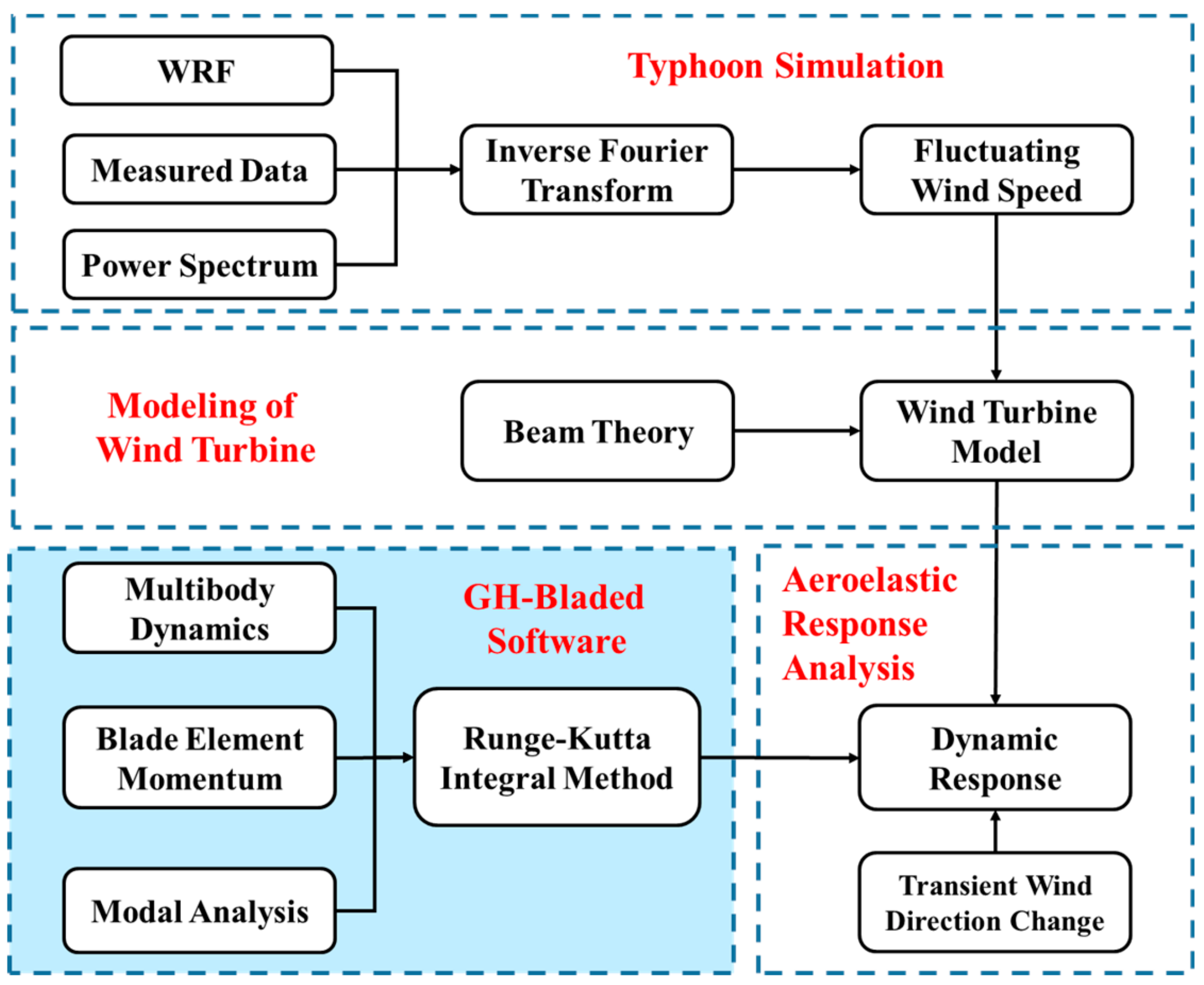
In order to obtain the pulsating wind speed inflow conditions required for WT dynamics calculation, the inverse Fourier transform method based on the stationary Gaussian process was used to perform time–frequency conversion of the power spectral density function [30]. The method can accurately simulate the wind speed field, which is consistent with the measured data, and includes the following two steps:

(1)

Knowing the pulsating power spectrum S(n) and the simulation time T, since the time history of pulsating wind speed has ergodic characteristics, the Fourier amplitude spectrum F(n) can be calculated via the following formula:

$$F\left(n\right)=\sqrt{T\cdot S\left(n\right)}.$$

(4)

(2)

The discrete Fourier transform is applied to the complex sequence F(n); t is the real component which determines the pulsating wind speed:

$$v\left(t\right)=real[IDFT(\sqrt{T\cdot S\left(n\right)})].$$

(5)

Considering that the WT blade is a flexible structure with a high slenderness ratio, the spatial correlation of each simulated node in the wind field needs to be considered when generating the pulsating wind speed [31]. The related function can be expressed as:

$$coh\left(i,k\right)=e^{(-\frac{\left|z_i-z_k\right|}{L_z})},$$

(6)

where |z_i-z_k| is the distance between two points in the vertical direction, and L_z is the vertical turbulence integral scale.

In this study, the aerodynamic load, modal analysis, and structural dynamic response of WTs in a typhoon were performed using the GH-BLADED commercial software package [28], which proved its high calculation accuracy and reliability in the performance analysis of many kinds of WTs. The unsteady blade element momentum theory was used in the aerodynamic calculation, adding the dynamic inflow and stall models for the unsteady aerodynamic effects [32,33,34]. The description of the structural dynamics was based on a modal model, using the Floquet analysis method to determine the modal properties of periodic systems. The equation of motion is expressed as follows:

$$\left[M\right]\ddot{q}\left(t\right)+\left[C\right]\dot{q}\left(t\right)+\left[K\right]q\left(t\right)=F\left(t\right),$$

(7)

where M, C, K are mass, damping, and stiffness matrices, respectively, while q and F are the modal and modal force vectors, respectively. By transforming the above formula into a generalized eigenvalue form and normalizing it, the decoupled dynamic equation in the modal space can be obtained:

$$\ddot{x}\left(t\right)+2{\omega }_i{\xi }_i\dot{x}\left(t\right)+{\omega }_i^{2}x\left(t\right)={\varphi }_i^{T}F\left(t\right),$$

(8)

where ${\omega }_i$ and ${\varphi }_i$ are the i-th natural frequency and vibration mode of the system, respectively, while ${\xi }_i$ is the damping ratio. In the solving process, the tower, blade, and hub coordinate systems were established to derive the main components of the WT, and then the equations of each order were solved one by one. The variable-step fourth-order Runge–Kutta numerical integration method was used to perform time-stepping of the differential equations to obtain the response of each mode, which realizes the coupling of aerodynamics and structure [35,36,37,38].

3. Analysis of Calculation Results

3.1. Wind Turbine Model

As a case study of a WT under typhoon conditions, a commercial 6 MW offshore WT was selected, the main parameters of which are listed in

Table 2. Main parameters of the 6MW wind turbine [25].

Technical Parameter	Value	Technical Parameter	Value
Rated wind speed, m/s	10	Hub height	100 m
Number of blades	3	Blade length	78 m
Windwheel diameter, m	160.7 m	Tip prebending	10 m
First-order natural frequency (out of plane)	0.508 Hz	First-order natural	0.826 Hz
		frequency (in plane)
Second-order natural frequency (out of plane)	1.364 Hz	Second-order natural	2.565 Hz
		frequency (in plane)
Tower first-order natural frequency, Hz	0.217 Hz	Second-order natural	1.321 Hz
		Frequency of tower

[25].

The simulation range of the WT inflow wind speed field is 200 m × 200 m, which is divided into 256 nodes covering the entire wind wheel plane, as shown in Figure 4. The WT blade 1 is defined as being vertically upward, while blades 2 and 3 are inclined clockwise by 120 degrees in sequence. As controls of typhoon wind, the normal winds representing normal atmospheric conditions were obtained by Kaimal spectrum specified in the IEC 61400 standard. The pulsating wind simulation time is 10 min according to the above standard.

The pulsating wind simulation time is 10 min, according to the IEC 61400 standard. As a reference, the normal wind conditions (without sudden changes of the wind direction) were also simulated using the Kaimal spectrum specified in the above standard.

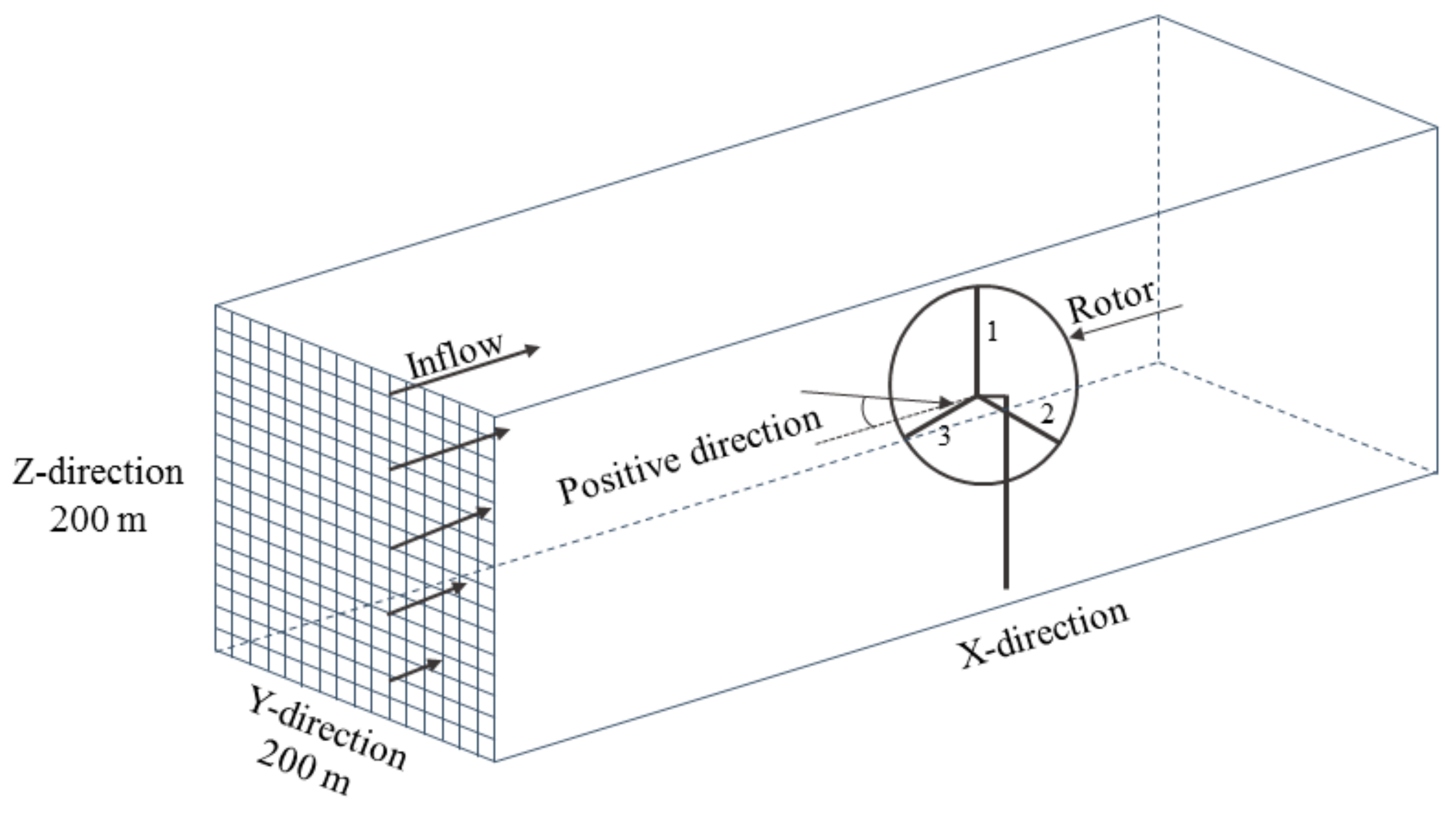
3.2. Analysis of Wind Characteristics

Figure 5 and Figure 6 show comparisons of wind speed and direction, respectively, with measured data within 24 h of the typhoon simulation using the WRF model. The location is (111.4° E, 21.45° N), and the height is 70 m. The simulated average wind speed and direction variation agree well with the measured trends. Within 24 h, the wind speed exhibited an “M” type distribution, while the wind direction changed by nearly 200°. Both simulated and measured maximum wind speed values occur at 8 h, and their difference (error) is 3.9%. Considering the complex dynamic and thermal characteristics of a typhoon, this is an acceptable simulation result. According to the nonlinear least squares’ method, the curve of the typhoon’s near-surface wind profile at this time was fitted, as shown in Figure 7. Since the position of the measuring point is at sea, the index rate parameter is small, namely 0.06257.

Figure 8 shows a comparison of the results of the pulsating power spectra in three directions. The generated spectrum fluctuates around the target spectrum without a large deviation. The X- and Z-directions contain the highest and lowest pulsating energies, respectively. In order to compare the differences between typhoon and normal wind, the pulsating wind in a normal atmospheric environment was also calculated in combination with the Kaimal spectrum, whose parameters were fitted by many cases under normal wind conditions. Figure 9 shows the comparison between the simulated and measured turbulence intensity at the hub height. The results simulated by the proposed spectrum are in good agreement with the measured ones. The X-direction error that has the greatest impact on WT dynamics simulation is only 1.7%, which is significantly better than the simulation results based on the Kaimal spectrum.

The pulsating wind is a non-stationary process with high randomness; thus, the simulations of pulsating wind were carried out 10 times to compare the vortex scale differences between the typhoon and normal wind. The turbulent integral scale is the vortex scale in the pulsating wind, which can be calculated by the following formula:

$$L_{ux}=\frac{U}{{\sigma }_u^2}{{\displaystyle \int }}_0^{\infty }{R}_u\left(\tau \right)d\tau ,$$

(9)

where L_ux is the turbulent integral scale in the x-direction, σ_u is the variance of the pulsating velocity in this direction, and R_u(τ) is the autocorrelation function. Figure 10 shows the turbulent integral scale in three directions at the hub height, in which the x-coordinate represents the number of simulations, and L_ux, L_uy, and L_uz represent the turbulent integral scale in the x, y, and z directions, respectively. The vortex scale in the typhoon is generally larger than in normal wind. The vortex change in the X-direction is the most significant, and those in the two other directions change more gently.

3.3. Analysis of Aeroelastic Response

Three scenarios were set up to study the aeroelastic response characteristics of WTs under a typhoon. The average wind speed of scenario 1 was specified according to the Hagupit typhoon simulation results, which was 24.4 m/s (9 h in Figure 5). At this time, the WT was running normally, and the average speed was 9.5 rpm. The average wind speed of the incoming flow of scenario 2 was 25.3 m/s (8 h in Figure 5), at which time the WT was in the state of shutdown and feathering. The average wind speed of scenario 3 was set to 40 m/s, which represents the severe typhoon conditions. At this time, the WT was also in the state of shutdown and feathering.

Figure 11 shows the time-history comparison of the tip vibration response of blade 1 in the main force directions of the three scenarios. Under normal operating conditions, the flapping direction (X-direction) of the blade is the main force direction. After the shutdown, the blade was feathering to 90°, so the main force direction changed to the direction of the shimmy (Y-direction). It can be seen that when the WT was in normal operation, whether it was under a typhoon or a normal wind, the blade tip vibration scope exceeded 30 m under the excitation of an average wind speed of 24.4 m/s. The tip response in a typhoon was 14.4% higher than that of in normal wind, which also proves the special wind characteristics of the typhoon. In the two shutdown scenarios, the vibration scopes of the blade were significantly reduced. In the typhoon, the blade tip vibration scopes were 7.92 and 13.09 m at the average wind speeds of 25.3 and 40 m/s, respectively, which is significantly higher than 3.16 and 9.39 m under the normal wind conditions. This implies that the typhoon will induce large-scale vibrations, in contrast with the normal wind.

In order to study the influence of the sudden change of typhoon wind direction on the vibration characteristics of the wind turbine, four cases were considered under each scenario, which represented the WT inflow without wind direction change, and the sudden changes in wind direction in 6 s of 30, 60, and 90 degrees, respectively. Figure 12 shows the response time history of the tip of blade 1 for different wind direction fluctuations in three scenarios, and the durations of sudden wind direction changes are shown in the dotted rectangle. In the absence of wind direction fluctuation in scenario 1, the response of the blade is approximately periodic. As the fluctuation angle of the wind direction increases, the scope increases. The scope is increased by 27.9% when the wind direction fluctuation is 90°, as compared to that with no wind direction fluctuation. It should be noted that at the 90° wind direction fluctuation, the maximum deformation of the tip in the positive direction of the X-axis reaches 28.4 m. This seriously exceeds the safety threshold for the headroom in the design standard and poses a serious threat to the safety of the WT.

Under the two shutdown scenarios, the vibration scope of the blade also gradually increases as the direction change angle is increased. At an average wind speed of 25.3 m/s and 40 m/s, the vibration scopes of the blades are 12.7 m and 19.4 m, respectively; when the wind direction is abruptly changed by 90°, which are 2.5 and 3.5 times, respectively, of the case without wind direction fluctuation. It can be concluded from the above analysis that a sudden change in wind direction in the typhoon will greatly increase the vibration scope of the WT blade. The vibration amplitudes of the blades are up to 28.4, 8.2, and 15.5 m in average wind speeds of 24.4, 25.3, and 40 m/s, respectively, when the wind direction is abruptly changed by 90°. The WT has the largest increase in vibration amplitude when the wind speed is close to 25 m/s, so early protection measures, such as early shutdown, should be applied to the WT under typhoon conditions.

Figure 13 and Figure 14 show the frequency domain response of the WT blade in normal operation (scenario 1) and shutdown (scenario 2) conditions. The first vibration peak under the two conditions corresponds to the first-order natural frequency of the tower, indicating that the vibration characteristics of the WT blade are closely related to its components. From the perspective of energy change, the peak energy of the blade vibration during normal operation of the WT is significantly higher than that in the shutdown state. However, a sudden change in the wind direction has little effect on its amplitude and the corresponding frequency, while the peak amplitude of the shutdown state obviously increases, and the high-frequency energy begins to increase. This indicates that the wind direction fluctuation has a significant impact on the energy distribution.

4. Conclusions

In this paper, the mesoscale WRF model was used to simulate the typhoon average wind speed field evolution. The pulsating wind speed field with the characteristics of typhoon Hagupit (2008) was simulated by the measured power spectrum and inverse Fourier transform. The WT structural model was constructed based on the modal method and beam theory. The GH-BLADED software was used to calculate the aerodynamic load and aeroelastic response via the proposed method for calculating the dynamic response of WTs during the typhoon’s evolution period. Based on this method, the aeroelastic response characteristics of a 6 MW offshore WT under different wind speeds and directional fluctuation in a typhoon were analyzed. The main conclusions are as follows:

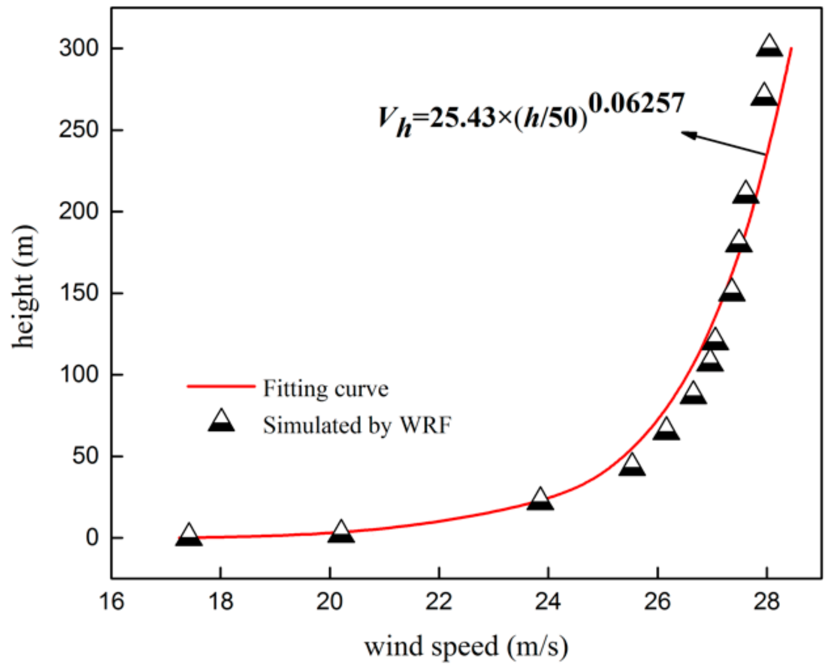
• An entire process simulation of the typhoon Hagupit (Nina) was carried out, and the wind speeds and wind direction changes within 24 h were compared with the measured values. It was found that the simulated average wind speeds and directional fluctuations agreed well with the measured trend; the wind speed exhibited an “M” type distribution within the specified 24 h, and the wind direction changed by nearly 200°. The maximum error between simulated and measured wind speeds was 3.9%. The wind profile index was as small as 0.06257 and complied with the observations. This indicates that the results of the typhoon’s average wind speed field obtained based on the WRF model are reliable.
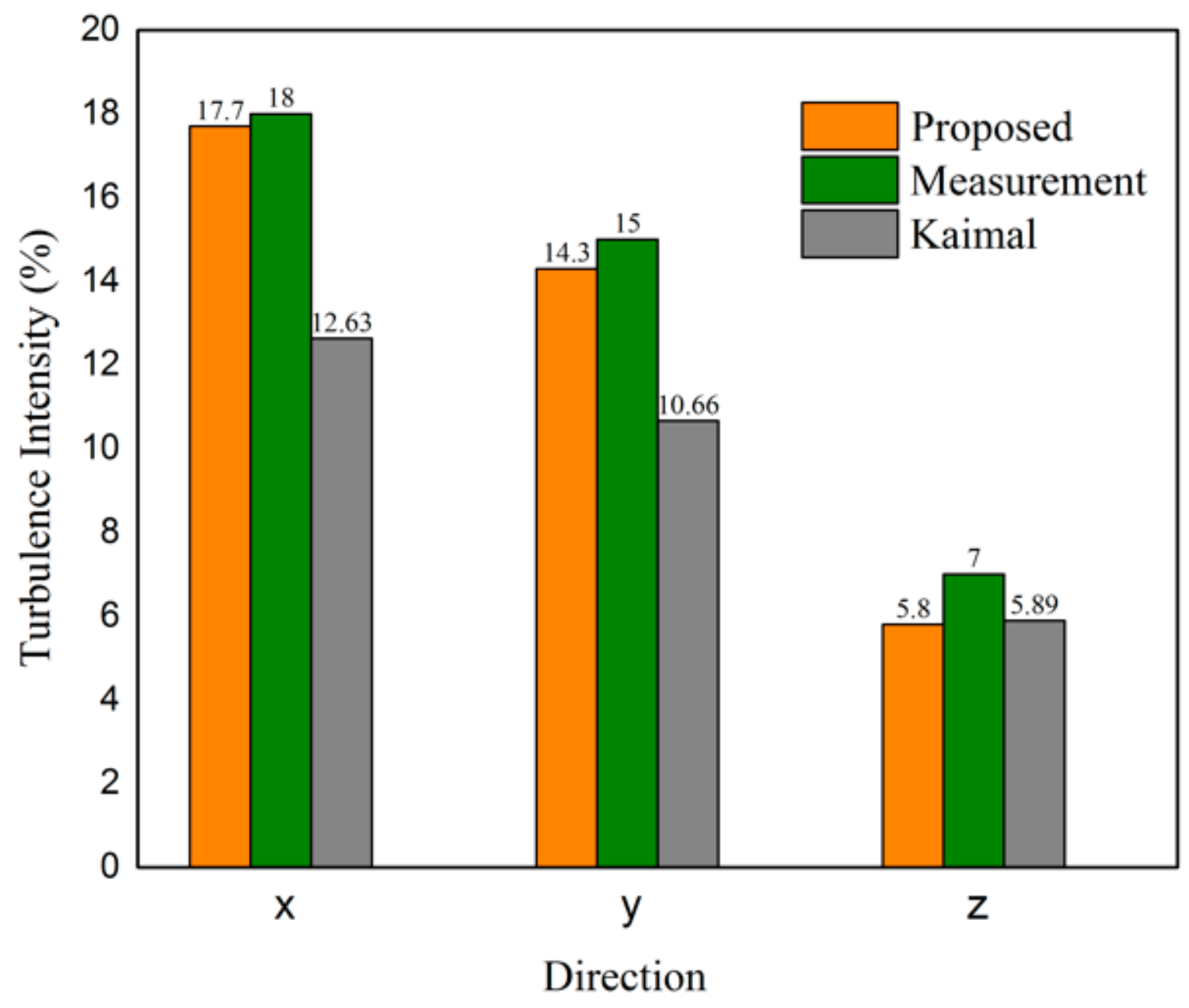
• The coupled wind power spectrum method and the inverse Fourier transform method were jointly applied to generate the typhoon’s pulsating wind speed, which had turbulence characteristics which were close to the measured values. The turbulence intensity error in the X-direction, which had the greatest influence on the vibration of the WT blade, was only 1.7%, which outperformed that derived via the Kaimal spectrum. The simulation results show that the turbulent vortex scale in a typhoon is generally higher than that of a normal wind.
• Under typhoon and normal wind conditions, the aeroelastic responses of the WT at the average wind speeds of 24.4, 25.3, and 40 m/s were analyzed. The tip vibration scope responses in the typhoon exceeded those of the normal wind by 14.4%, 150.1%, and 39.4%, respectively. In addition, the vibration amplitude of the WT under normal operation was significantly higher than that under shutdown conditions.
• The vibration scope of the WT blade increases with wind direction fluctuation. When the latter reached 90° under normal operating conditions, the vibration scope increased by 27.9%, as compared to zero fluctuation. In particular, the maximum blade tip deflection in the X-axis direction reached 28.4 m, which seriously exceeded the safety threshold of the design standard. Therefore, early protection measures, such as early shutdown, should be applied to the WT under the typhoon conditions.

References

- Li, Q.S.; Li, X.; He, Y.C.; Yi, J. Observation of wind fields over different terrains and wind effects on a super-tall building during a severe typhoon and verification of wind tunnel predictions. J. Wind Eng. Ind. Aerodyn. 2017, 162, 73–84. [Google Scholar] [CrossRef]
- Hazelton, A.T.; Rogers, R.F.; Hart, R.E. Analyzing simulated convective bursts in two Atlantic hurricanes. Mon. Weather Rev. 2017, 145, 3073–3094. [Google Scholar] [CrossRef]
- Kepert, J.D. Time and space scales in the tropical cyclone boundary layer and the location of the eyewall updraft. J. Atmos. Sci. 2017, 74, 1–53. [Google Scholar] [CrossRef]
- Williams, G.J. The thermodynamic evolution of the hurricane boundary layer during eyewall replacement cycles. Meteorol. Atmos. Phys. 2017, 129, 611–627. [Google Scholar] [CrossRef]
- Li, L.; Kareem, A.; Xiao, Y.; Song, L.; Zhou, C. A comparative study of field measurements of the turbulence characteristics of typhoon and hurricane winds. J. Wind Eng. Ind. Aerodyn. 2015, 140, 49–66. [Google Scholar] [CrossRef]
- Cao, S.; Tamura, Y.; Kikuchi, N.; Saito, M.; Nakayama, I.; Matsuzaki, Y. Wind characteristics of a strong typhoon. J. Wind Eng. Ind. Aerodyn. 2009, 97, 11–21. [Google Scholar] [CrossRef]
- Dai, K.S.; Sheng, C.; Zhao, Z. Nonlinear response history analysis and collapse mode study of a WT tower subjected to tropical cyclonic winds. Wind Struct. 2017, 25, 79–100. [Google Scholar]
- Han, T.; McCann, G.; Freudenreich, K. How can a WT survive in a tropical cyclone? Renew. Energy 2014, 70, 3–10. [Google Scholar] [CrossRef]
- Chen, X.; Li, C.F. Failure investigation on a coastal wind farm damaged by super typhoon: A forensic engineering study. J. Wind Eng. Ind. Aerodyn. 2015, 147, 132–142. [Google Scholar] [CrossRef]
- Chen, X.; Xu, J.Z. Structural failure analysis of WTs impacted by super typhoon Usagi. Eng. Fail. Anal. 2016, 36, 391–404. [Google Scholar] [CrossRef]
- Chen, X.; Li, C.F.; Tang, J. Structural integrity of WTs impacted by tropical cyclones: A case study from China. J. Phys. Conf. Ser. 2016, 753, 1–12. [Google Scholar] [CrossRef]
- Zhang, Z.H.; Li, J.H.; Zhuge, P. Failure analysis of large-scale wind power structure under simulated typhoon. Math. Probl. Eng. 2003, 4, 30–32. [Google Scholar] [CrossRef] [Green Version]
- Liu, X.X.; Deng, Z.W.; Gao, Q.F. Typhoon-resistance analysis of WTs with different towers based on the time-domain method. J. Hunan Univ. 2017, 44, 82–88. [Google Scholar]
- Bangga, G.; Guma, G.; Lutz, T. Numerical simulations of a large offshore WT exposed to turbulent inflow conditions. Wind Eng. 2018, 42, 88–96. [Google Scholar] [CrossRef]
- Vickery, P.J.; Masters, F.J.; Powell, M.D.; Wadhera, D. Hurricane hazard modeling: The past, present, and future. J. Wind Eng. Ind. Aerodyn. 2009, 97, 392–405. [Google Scholar] [CrossRef]
- Wyszogrodzki, A.A.; Miao, S.; Chen, F. Evaluation of the coupling between mesoscale WRF and LES-EULAG models for simulating fine-scale urban dispersion. Atmos. Res. 2012, 118, 324–345. [Google Scholar] [CrossRef]
- Bauer, P.; Thorpe, A.; Brunet, G. The quiet revolution of numerical weather prediction. Nature 2015, 525, 47–55. [Google Scholar] [CrossRef] [PubMed]
- Reeves, H.; Snyder, C.; Rotenone, R. Prediction of landfalling hurricanes with the advanced hurricane WRF model. Mon. Weather Rev. 2008, 136, 1990–2005. [Google Scholar]
- Xiao, Q.N.; Zhang, X.Y.; Davis, C.; Tuttle, J.; Holland, G. Experiments of hurricane initialization with airborne Doppler radar data for the advanced research hurricane WRF (AHW) model. Mon. Weather Rev. 2009, 137, 2758–2777. [Google Scholar] [CrossRef]
- Huang, M.F.; Wang, Y.F.; Lou, W.J.; Cao, S.Y. Multi-scale simulation of time-varying wind fields for Hangzhou Jiubao Bridge during Typhoon Chan-Hom. J. Wind Eng. Ind. Aerodyn. 2018, 179, 419–437. [Google Scholar] [CrossRef]
- Liu, D.H.; Song, L.; Li, G.P. Study on wind profile of typhoon Hagupit using wind observed tower and wind profile radar measurements. J. Trop. Meteorol. 2011, 27, 317–326. [Google Scholar]
- Germanischer, L. Guideline for the Certification of WTs 2010 Edition; Brooktorkai 18, 20457; Brooktorkai: Hamburg, Germany, 2010; pp. 131–174. [Google Scholar]
- Dai, L.P.; Zhou, Q.A.; Zhang, Y.W. Analysis of WT blades aeroelastic performance under yaw conditions. J. Wind Eng. Ind. Aerodyn. 2017, 171, 273–287. [Google Scholar] [CrossRef]
- Dong, X.F.; Lian, J.J.; Wang, H.J. Structural vibration monitoring and operational modal analysis of offshore WT structure. Ocean Eng. 2018, 150, 280–297. [Google Scholar] [CrossRef]
- Han, R.; Wang, L.; Wang, T.G.; Gao, Z.T.; Wu, J.H. Study of dynamic response characteristics of the WT based on measured power spectrum in the eyewall region of typhoons. Appl. Sci. 2019, 9, 1–14. [Google Scholar]
- Kaimal, J.C.; Wyngaard, J.C.; Izumi, Y.; Coté, O.R. Spectral characteristics of surface-layer turbulence. Q. J. R. Meteorol. Soc. 1972, 98, 563–589. [Google Scholar] [CrossRef]
- Tony, B.; David, S.; Nick, J.; Ervin, B. Wind Energy; John Wiley & Sons, Ltd.: Hoboken, NJ, USA, 2001. [Google Scholar]
- Li, L.X.; Xiao, Y.Q.; Kareem, A.; Song, L.; Qin, P. Modeling typhoon wind power spectra near sea surface based on measurements in the South China sea. J. Wind Eng. Ind. Aerodyn. 2012, 104, 565–576. [Google Scholar] [CrossRef]
- Xu, Y.L.; Zhu, L.D. Buffeting response of long-span cable-supported bridges under skew winds. Part 2, Study. J. Sound Vib. 2005, 281, 675–697. [Google Scholar] [CrossRef]
- Rossi, R.; Lazzari, M.; Vitaliani, R. Wind field simulation for structural engineering purposes. Int. J. Numer. Methods Eng. 2004, 61, 738–763. [Google Scholar] [CrossRef]
- Shiotani, M.; Avai, H. Honorary Advisory Council for Scientific and Industrial Research. In Proceedings of the International Research Seminar on Wind Effects on Buildings and Structures, Ottawa, ON, Canada, 11–15 September 1967; pp. 535–555. [Google Scholar]
- Glauert, H. Airplane Propellers; Dover Publications: New York, NY, USA, 1963. [Google Scholar]
- Prandtl, L.; Betz, A. Vier Abhandlungen zur Hydrodynamik und Aerodynamik; Göttinger Nachr: Göttingen, Germany, 1927; pp. 88–92. [Google Scholar]
- Leishman, J.G.; Beddoes, T.S. A semi-empirical model for dynamic stall. J. Am. Helicopter Soc. 1989, 34, 3–17. [Google Scholar]
- Gao, Y.W.; Li, C.; Cheng, X. Research on foundation response of a tri-floater offshore WT. Conf. Ser. Mater. Sci. Eng. 2013, 52, 66–71. [Google Scholar]
- Rezaei, M.M.; Behzad, M.; Haddadpour, H. Aeroelastic analysis of a rotating WT blade using a geometrically exact formulation. Nonlinear Dyn. 2017, 84, 2367–2392. [Google Scholar] [CrossRef]
- Ho, J.Y.L. Direct path method for flexible multibody spacecraft dynamics. J. Spacecr. Rocket. 2012, 14, 102–110. [Google Scholar] [CrossRef]
- Bossanyi, E.A. GH Bladed Theory Manual; Garrad Hassan and Partners: Bristol, UK, 2009; pp. 13–19. [Google Scholar]