Assessment of Formal Credit and Climate Change Impact on Agricultural Production in Pakistan: A Time Series ARDL Modeling Approach

Abstract

This study attempts to investigate the short-run and long-run impact of formal credit (CR) and climate change (CC, via CO₂ emissions) on agricultural production (AP) in Pakistan. In addition, other imperative control variables included in this study comprise technology factors (tractors (TRs) and tube wells (TWs), energy consumption (EC), and labor force (LF). This study used annual data covering the period 1983–2016. The autoregressive distributed lag (ARDL) approach is applied to explore the cointegration between the underlying variables and used the granger causality test under the vector error correction model (VECM) context to determine the direction of causality among the variables. The findings of the ARDL bounds-testing approach suggest that there is a long-term relationship among formal credit, climate change (CO₂ emissions), technology factors (tractors and tube wells), energy consumption, labor force, and agricultural production. The empirical results reveal that formal credit, technology use (tractors), and labor force have a positive and significant impact on agricultural production in both the short-run and long-run. CO₂ emissions have a positive impact on agricultural production but are not significant in either case. Finally, a unidirectional relationship is established from formal credit to agricultural production; labor force to agricultural production; and electricity consumption and technology factors (tractors and tube wells) to CO₂ emissions. The recent study claims that formal institutions should guarantee the redeployment of their services/amenities to those who call for them acutely, with the purpose of boosting their approach to monetary credit facilities and empower farmers to further the resilience that will capitalize on post-fruitage enrichments. Finally, considering that climatic change is a widespread fact with regional community trajectories, perhaps the global community may provide reassurance for loaning to smallholder agriculturalists through central and commercial banks by protecting the moneys that banks lend to the agriculturalists towards supporting climatic change espousal strategies.

1. Introduction

The agriculture sector of Pakistan possess a dominant role in its economy, with a contribution to economic growth between 1949 and 1950 of about 60%, a decline of around 30% between 1978 and 1979, and ratio of about 18.5% during 2018–2019. However, its agriculture still plays a vigorous role in the economic sector as well as in rural development. The agriculture sector comprises five sub-sectors (e.g., major and minor crops, livestock, forestry, and fisheries, respectively). In 2018–2019, the growth rate of the agriculture sector was recorded as 0.85%, compared with 3.94% during 2017–2018. The growth of major crops in 2018–2019 was −6.55% and 1.95% for minor crops against growths in 2017–2018 of 3.56% and 6.15%, respectively. Moreover, other sub-sectors such as livestock, fishery, and forestry achieved growth rates of 4.00%, 0.79%, and 6.47%, respectively [1].

In Pakistan, the total cropped area is about 22 million hectares. Out of the total cropped area 9.18 million hectares (41.73%) are under wheat cultivation, 2.96 million hectares (13.45%) are for cotton cultivation, 2.89 million hectares (13.14%) are for rice cultivation, 1.13 million hectares (5.14%) are for maize cultivation, and 1.14 million hectares (5.18%) are for sugarcane cultivation. About 17.30 million hectares (78.64%) are covered by these five major crops. Further, 4.70 million hectares (21.36%) are covered by other crops [2]. Agricultural production and its growth in Pakistan is very low as compared with other emerging economies. To boost agricultural production, Pakistan needs to appropriately utilize fertilizers, pesticides, the adoption of improved varieties, modern technology, and irrigation, which required formal credit to support rural households for better production [3].

The utilization and role of formal credit are necessary in the farming sector. In recent decades, traditional farming transformations to modern commercialization farming have demanded adequate formal credit [4]. In Pakistan, during the period of 2018–2019, five major banks, 15 domestic private banks, and 10 microfinance banks jointly disbursed agricultural credit of PKR 804.9 billion, which represented 64.4% of the annual benchmark of PKR 1250.0 billion [1]. Khan and Hussain [5] stated that different sources of formal credit in Pakistan support farmers. The formal credit sources are still unable to extend ample agricultural credit to farmers, particularly to small-scale farmers.

Furthermore, the study concluded that formal education and landholding size positively and statistically affected the formal credit demand while credit sources, distance of credit sources from the farmhouse, and bribe and transaction costs negatively influenced the demand for formal credit. The major issue to obtaining credit from formal sources is that small-scale farmers face strict conditions and lending procedures. The cost of agricultural credit is very high, particularly for smallholder farmers who need certain amounts of agricultural loans from formal sources. The smallholder farmers have la ack of social capital and also have no material collateral [6]. As a result, small-scale farmers who are facing problems regarding accessibility of formal agricultural loans from formal sources resort to demanding agricultural credit from informal sources to fulfill their credit needs.

In the agriculture sector, formal agricultural credit is not a direct instrument to enhance crop productivity but it can assist smallholders to reduce their financial constraints in applying improved farming practices. Park et al. [7] stated that formal agricultural credit access is an antipode to poverty reduction among smallholders. Similarly, Adejobi and Atobatele [8] concluded that crop productivity and rural development can be derived on a sustained basis if the formal agricultural credit is sufficiently supplied to rural households in contravening the vicious cycle of poverty. In Pakistan, based on the survey data, many studies have been prepared to evaluate the influence of formal agricultural credit on crop efficiency [3,9,10,11,12], while annual time series data have resulted in a few studies that explored the influence of institutional credit on agricultural output [13,14,15].

Climate change (CC) is essentially attributed to the unabated rise in greenhouse gasses (GHGs), which bring fluctuations in temperature and rain patterns, and which negatively affect natural resources. Although this is a global phenomenon, the effects of CC on the agricultural production of developing countries is especially devastating [16,17,18,19,20]. In Pakistan, agricultural production is adversely affected because of CC and its low adaptive capacity [21,22]. The global climate risk index (GCRI) ranked Pakistan among the list of nations most affected due to CC and dangerous weather actions. The impact of CC is very important, as a significant portion of Pakistan’s inhabitants are directly or secondarily linked with the agriculture sector [23,24,25]. Similarly, poverty rates are still high in many developing countries, and climate change might result in poor crop yields and quality, losses of crops and revenue, intensifications in pest attacks, and interruptions in planting periods [16,26].

All these factors add fuel to the fire, causing severe financial and food security issues in the developing world. Therefore, a detailed investigation of climate change and the role of credit in coping with productivity issues in Pakistan can help policymakers support local farmers and permit them to deal with agriculture productivity problems. This study used the ARDL approach to assess the short- and long-term impacts of formal credit and carbon dioxide (CO₂) emissions on agricultural production in Pakistan from 1983 to 2016. To verify the robustness of the long-term relationships among the variables, we also employed a multivariate Johansen and Juselius [27] cointegration method. A granger causality test under a VECM context was applied to evaluate short-term connectedness. The current study is different from previous studies as it comprehends climatic issues, formal credit, and agricultural production in Pakistan for the first time in a broad way.

The paper is divided into five sections. Following the introduction, a theoretical and empirical literature review is conducted in Section 2, a data and methodological road map is presented in Section 3, and Section 4 outlines the results along with a discussion. Lastly, the final concluding outlines, recommendations, and study implications are constructed in Section 5.

2. Review of Literature

Crop productivity is low in Pakistan when compared with developed economies. This is due to small landholding sizes, the application of outdated approaches to farming, poor irrigation systems, and a poor adoption of up-to-date agricultural technologies [3,4], all of which result in the small savings or low-income levels of rural households. Consequently, formal financial intuitions need to offer financial support so that farmers can adopt and use more-advanced farm practices. Formal agricultural credit plays a central role in boosting crop production. Easy accessibility and the timely availability of agricultural credit enables rural households to purchase farming inputs including seeds, chemical fertilizers, pesticides, and other implements. Rural households are dependent on formal as well informal credit channels to meet credit demands [28,29].

Presently, the demand for formal agricultural credit is rapidly increasing in farming sectors due to the expansion of farm inputs. Formal agricultural credit is known to be an imperative instrument for boosting agricultural production and improving smallholder farmers’ living standards. Short- and long-term loans take a major toll on crop outputs. Both types of loans increase agricultural productivity and also improve rural household incomes. Short-term and long-term loans, therefore, are an essential part of the modern agriculture sector. Several empirical studies have been documented regarding the effects of credit on crop productivity; for instance, [14,15,30,31,32,33,34,35,36,37,38] reported that formal agricultural loans have a significant effect on crop productivity. In developing economies, farm credit is an essential tool for enhancing agricultural productivity [4,33,39,40].

The role of rural financial credit markets in food production has been documented internationally. In Pakistan, the significance of rural financial credit markets has been noted for boosting up the yields of major crops including rice, wheat, sugarcane, maize, and cotton, as well as for improving the socio-economic situations of the framers [37,41]. Dong et al. [42] examined the impact of credit constraints on rural household productivity by using the field survey data of 511 rural farm households in China. An econometric ordinary least squares (OLS) method was applied in order to analyze the data. The empirical results showed that an average agricultural output was enhanced by 75%. Thus, farmer characteristics, labor participation, and formal education cannot be fully functional without coordination and proper participation.

Obilor [43] reported that formal loans have a substantial effect on agricultural development. Bashir et al. [11] explored the heterogeneous impacts of formal credit on outputs of sugarcane crop in Faisalabad, Pakistan by means of field survey information of 114 farmers. Findings revealed that formal credit has a positive impact on sugarcane production. Rahman et al. [44] observed the impacts of agricultural loans on agricultural production in Pakistan by utilizing the field survey information of 300 agriculturalists. The empirical results showed that both short- and long-term loans, household income, household size, and education have positive and significant impacts on agricultural production. A study in Pakistan by Ahmad et al. [9] discovered the effect of formal agricultural credit on wheat crop yields using primary data collected from 160 farmers. The findings exhibited that credit has a positive effect on wheat productivity. The authors also reported that only 30% of farmers utilized credit for the purchase of farming inputs, while 70% of farmers utilized credit for other purposes.

Rehman et al. [45] assessed the heterogeneous effects of farming inputs along with formal credit on farming efficiency in Pakistan from 1978 to 2015. The Johansen co-integration testing and OLS method were applied for the estimations. The estimated outcomes revealed that seeds, formal credit and fertilizers used have a positive significant effect on agricultural productivity. Ayaz et al. [10] discovered the impacts of formal agrarian loans on productivity in Pakistan using the survey data of 300 agrarians. Results exhibited that formal agricultural loans have a substantial influence on farmers’ practical efficacy. Jan and Manig [46] found that formal agricultural loans disbursed by Zarai Taraqiati Bank Limited (ZTBL) showed a positive significant effect on field crop production in Pakistan.

By examining the effect of climate change (CC) on the credit needs of Nigerian farmers, Abraham and Fonta [26] confirm that high temperature, lengthy dry periods, floods, and deficiencies lead to truncated harvesting and less income. Climate change significantly affects credit needs, but the 96% of farmers have no access to the credit facilities needed to reduce this impact. Furthermore, timely credit availability can reduce low harvest crop loss and contribute to the wellbeing of farmers. Bangladesh is very susceptible to the effects of CC and adaptation is emerging as a key policy response. Formal institutions and linked communities play a key role in building place-based capacities for mitigation and adaptation strategies in the farming sector. Additionally, the increased incorporation of cultural mechanisms and partnerships with more community-based informal institutions can improve overall benefits [47].

Assessing the impact of CC on cereal production of China Zhou and Turvey [48] suggests that the effects of CC vary among regions and crops. Generally, the impact of warming on cereal production is always positive, and that most provinces in central, western and northern China are less sensitive to climate variables due to adaptation; however, eastern provinces (namely, Shandong and Hebei) are very vulnerable. Investigating the heterogeneous impacts of CC on the major crops of Pakistan, Ali et al. [21] determined that extreme temperature have a negative impact on the production of wheat, while minimum temperatures have an encouraging effect on all kinds of crops. Similarly, rainfall negatively affects the yield of certain crops, excluding wheat. To ensure food security and mitigate the adverse effects of CC, the study suggested that the improvement and expansion of heat- and drought-resistant varieties is necessary in the farming sector.

Exploring the adaptation of wheat farmers to CC and its effects on food production, Abid et al. [23] suggested that adapting wheat crops to CC has a positive effect on productivity. The main adaptation tactics included changing planting dates and adopting improved varieties and different types of fertilizer, but these strategies are not implemented at a large scale due to less awareness among rural farmers in Pakistan. On the contrary, exploring the impact of CC on wheat productivity in Pakistan, Janjua et al. [49] revealed that CC (CO₂ emissions) has not affected wheat productivity in the country. Nonetheless, appropriate measures are necessary to confront any adverse shock to wheat production in Pakistan. Considering the previous literature, an investigation on the nexus of formal credit, climate change, and agricultural productivity adds novel insight for policymakers looking to increase overall production.

3. Data and Methods

The time series data utilized in this study covers the 1983–2016 period, with agricultural production (AP) data represented in kg per hectare, labor force (LF) per one million, and CO₂ emissions (CO₂) in metric tons per capita; all the selected variables have been retrieved from the database of the World Bank [50]. Other factors include: formal credit (CR) proxied per capita for real formal agricultural loans disbursed to farmers by the financial sector per million Pakistani rupees; agricultural technology factors such as tractors (TRs) in numbers; tube wells (TWs) numbers per 1000; and consumption of electricity by the agricultural sector (EC) in Gwh. These have been collected from Economic Survey of Pakistan [1].

3.1. Model Specification

The present paper examines the impact of formal credit and climate change (CO₂ emissions) on agricultural production in Pakistan from 1983 to 2016. The empirical framework for this study is specified and the implicit form is as follows:

$$A{P}_t=f\left(C{R}_t,T{R}_t,T{W}_t,E{C}_t,L{F}_t,C{O}_{2t}\right)$$

(1)

The empirical study carries out the several estimation tests, thus Equation (1) can be articulated as follows:

$$\begin{array}{cc}\hfill LNA{P}_t={\alpha }_0 +& \hfill {\alpha }_{1}LNC{R}_t+{\alpha }_{2}LNT{R}_t+{\alpha }_{3}LNT{W}_t+{\alpha }_{4}LNE{C}_t+{\alpha }_{5}LNL{F}_t+{\alpha }_{6}LNC{O}_{2t}\\ \hfill & +{\epsilon }_t\hfill \end{array}$$

(2)

where $LNA{P}_t$ represents the logarithm function of the agricultural output; $LNC{R}_t$ represents the logarithm function of formal credit; $LNT{R}_t$ represents the logarithm function of the tractors; $LNT{W}_t$ represents the logarithm function of the tube wells; $LNE{C}_t$ represents the logarithm function of the consumption of electricity in agricultural sector; $LNL{F}_t$ represents the logarithm function of the laborr force; and $LNC{O}_{2t}$ represents the logarithm function of the CO₂ emissions, respectively.

3.2. Estimation Techniques

3.2.1. Autoregressive Distributed Lag (ARDL)

Our study used an autoregressive distributed lag (ARDL) method to evaluate the long- and short-run impacts of formal credit and climate change (CO₂ emissions) on agricultural production in Pakistan, which was originally presented by Pesaran et al. [51]. For empirical assessment, a number of studies from the literature were used, employing several cointegration approaches for different situations. The first cointegration approach was Engle and Granger [52], which is appropriate for any two study variables in I(1) order. The second cointegration approach was Johansen and Juselius [27], which can be applied for large sample sizes and any study variables consisting of an equal integration order. Both cointegration approaches have a few restrictions, limiting study variables to being stationary and having a similar integration order. The ARDL method is much more useful than other cointegration approaches, and offers trustworthy outcomes for small samples [53].

The ARDL bounds-testing models can be expressed as follows:

$$\begin{array}{ll}\Delta LNA{P}_t={\psi }_0+& {\displaystyle {\displaystyle \sum }_{i=1}^p}{\psi }_{1i}\Delta LNA{P}_{t-i}+{\displaystyle {\displaystyle \sum }_{i=1}^p}{\psi }_{2i}\Delta LNC{R}_{t-i}+{\displaystyle {\displaystyle \sum }_{i=1}^p}{\psi }_{3i}\Delta LNT{R}_{t-i}+{\displaystyle {\displaystyle \sum }_{i=1}^p}{\psi }_{4i}\Delta LNT{W}_{t-i}\\ & +{\displaystyle {\displaystyle \sum }_{i=1}^p}{\psi }_{5i}\Delta LNE{C}_{t-i}+{\displaystyle {\displaystyle \sum }_{i=1}^p}{\psi }_{6i}\Delta LNL{F}_{t-i}+{\displaystyle {\displaystyle \sum }_{i=1}^p}{\psi }_{7i}\Delta LNC{O}_{2t-i}+{\lambda }_{1}LNA{P}_{t-1}+{\lambda }_{2}LNC{R}_{t-1}\\ & +{\lambda }_{3}LNT{R}_{t-1}+{\lambda }_{4}LNT{W}_{t-1}+{\lambda }_{5}LNE{C}_{t-1}+{\lambda }_{6}LNL{F}_{t-1}+{\lambda }_{7}LNC{O}_{2t-1}\\ & +{\epsilon }_t\end{array}$$

(3)

$$\begin{array}{ll}\Delta LNC{R}_t={\psi }_0+& {\displaystyle {\displaystyle \sum }_{i=1}^p}{\psi }_{1i}\Delta LNC{R}_{t-i}+{\displaystyle {\displaystyle \sum }_{i=1}^p}{\psi }_{2i}\Delta LNA{P}_{t-i}+{\displaystyle {\displaystyle \sum }_{i=1}^p}{\psi }_{3i}\Delta LNT{R}_{t-i}+{\displaystyle {\displaystyle \sum }_{i=1}^p}{\psi }_{4i}\Delta LNT{W}_{t-i}\\ & +{\displaystyle {\displaystyle \sum }_{i=1}^p}{\psi }_{5i}\Delta LNE{C}_{t-i}+{\displaystyle {\displaystyle \sum }_{i=1}^p}{\psi }_{6i}\Delta LNL{F}_{t-i}+{\displaystyle {\displaystyle \sum }_{i=1}^p}{\psi }_{7i}\Delta LNC{O}_{2t-i}+{\lambda }_{1}LNC{R}_{t-1}+{\lambda }_{2}LNA{P}_{t-1}\\ & +{\lambda }_{3}LNT{R}_{t-1}+{\lambda }_{4}LNT{W}_{t-1}+{\lambda }_{5}LNE{C}_{t-1}+{\lambda }_{6}LNL{F}_{t-1}+{\lambda }_{7}LNC{O}_{2t-1}\\ & +{\epsilon }_t\end{array}$$

(4)

$$\begin{array}{ll}\Delta LNT{R}_t={\psi }_0+& {\displaystyle {\displaystyle \sum }_{i=1}^p}{\psi }_{1i}\Delta LNT{R}_{t-i}+{\displaystyle {\displaystyle \sum }_{i=1}^p}{\psi }_{2i}\Delta LNC{R}_{t-i}+{\displaystyle {\displaystyle \sum }_{i=1}^p}{\psi }_{3i}\Delta LNA{P}_{t-i}+{\displaystyle {\displaystyle \sum }_{i=1}^p}{\psi }_{4i}\Delta LNT{W}_{t-i}\\ & +{\displaystyle {\displaystyle \sum }_{i=1}^p}{\psi }_{5i}\Delta LNE{C}_{t-i}+{\psi }_6{\displaystyle {\displaystyle \sum }_{i=1}^p}{\psi }_{6i}\Delta LNL{F}_{t-i}+{\displaystyle {\displaystyle \sum }_{i=1}^p}{\psi }_{7i}\Delta LNC{O}_{2t-i}+{\lambda }_{1}LNT{R}_{t-1}\\ & +{\lambda }_{2}LNC{R}_{t-1}+{\lambda }_{3}LNA{P}_{t-1}+{\lambda }_{4}LNT{W}_{t-1}+{\lambda }_{5}LNE{C}_{t-1}+{\lambda }_{6}LNL{F}_{t-1}+{\lambda }_{7}LNC{O}_{2t-1}\\ & +{\epsilon }_t\end{array}$$

(5)

$$\begin{array}{ll}\Delta LNT{W}_t={\psi }_0+& {\displaystyle {\displaystyle \sum }_{i=1}^p}{\psi }_{1i}\Delta LNT{W}_{t-i}+{\displaystyle {\displaystyle \sum }_{i=1}^p}{\psi }_{2i}\Delta LNT{R}_{t-i}+{\displaystyle {\displaystyle \sum }_{i=1}^p}{\psi }_{3i}\Delta LNC{R}_{t-i}+{\displaystyle {\displaystyle \sum }_{i=1}^p}{\psi }_{4i}\Delta LNA{P}_{t-i} \\ & +{\displaystyle {\displaystyle \sum }_{i=1}^p}{\psi }_{5i}\Delta LNE{C}_{t-i}+{\displaystyle {\displaystyle \sum }_{i=1}^p}{\psi }_{6i}\Delta LNL{F}_{t-i}+{\displaystyle {\displaystyle \sum }_{i=1}^p}{\psi }_{7i}\Delta LNC{O}_{2t-i}+{\lambda }_{1}LNT{W}_{t-1}+{\lambda }_{2}LNT{R}_{t-1}\\ & +{\lambda }_{3}LNC{R}_{t-1}+{\lambda }_{4}LNA{P}_{t-1}+{\lambda }_{5}LNE{C}_{t-1}+{\lambda }_{6}LNL{F}_{t-1}+{\lambda }_{7}LNC{O}_{2t-1}\\ & +{\epsilon }_t\end{array}$$

(6)

$$\begin{array}{ll}\Delta LNE{C}_t={\psi }_0+& {\displaystyle {\displaystyle \sum }_{i=1}^p}{\psi }_{1i}\Delta LNE{C}_{t-i}+{\displaystyle {\displaystyle \sum }_{i=1}^p}{\psi }_{2i}\Delta LNT{W}_{t-i}+{\displaystyle {\displaystyle \sum }_{i=1}^p}{\psi }_{3i}\Delta LNT{R}_{t-i}+{\displaystyle {\displaystyle \sum }_{i=1}^p}{\psi }_{4i}\Delta LNC{R}_{t-i}\\ & +{\displaystyle {\displaystyle \sum }_{i=1}^p}{\psi }_{5i}\Delta LNA{P}_{t-i}+{\displaystyle {\displaystyle \sum }_{i=1}^p}{\psi }_{6i}\Delta LNL{F}_{t-i}+{\displaystyle {\displaystyle \sum }_{i=1}^p}{\psi }_{7i}\Delta LNC{O}_{2t-i}+{\lambda }_{1}LNE{C}_{t-1}+{\lambda }_{2}LNT{W}_{t-1}\\ & +{\lambda }_{3}LNT{R}_{t-1}+{\lambda }_{4}LNC{R}_{t-1}+{\lambda }_{5}LNE{C}_{t-1}+{\lambda }_{6}LNL{F}_{t-1}+{\lambda }_{7}LNC{O}_{2t-1}\\ & +{\epsilon }_t\end{array}$$

(7)

$$\begin{array}{ll}\Delta LNL{F}_t={\psi }_0+& {\displaystyle {\displaystyle \sum }_{i=1}^p}{\psi }_{1i}\Delta LNL{F}_{t-i}+{\displaystyle {\displaystyle \sum }_{i=1}^p}{\psi }_{2i}\Delta LNE{C}_{t-i}+{\displaystyle {\displaystyle \sum }_{i=1}^p}{\psi }_{3i}\Delta LNT{W}_{t-i}+{\displaystyle {\displaystyle \sum }_{i=1}^p}{\psi }_{4i}\Delta LNT{R}_{t-i}\\ & +{\displaystyle {\displaystyle \sum }_{i=1}^p}{\psi }_{5i}\Delta LNC{R}_{t-i}+{\displaystyle {\displaystyle \sum }_{i=1}^p}{\psi }_{6i}\Delta LNA{P}_{t-i}+{\displaystyle {\displaystyle \sum }_{i=1}^p}{\psi }_{7i}\Delta LNC{O}_{2t-i}+{\lambda }_{1}LNL{F}_{t-1}+{\lambda }_{2}LNE{C}_{t-1}\\ & +{\lambda }_{3}LNT{W}_{t-1}+{\lambda }_{4}LNT{R}_{t-1}+{\lambda }_{5}LNC{R}_{t-1}+{\lambda }_{6}LNA{P}_{t-1}+{\lambda }_{7}LNC{O}_{2t-1}\\ & +{\epsilon }_t\end{array}$$

(8)

$$\begin{array}{ll}\Delta LNC{O}_{2t}={\psi }_0+& {\displaystyle {\displaystyle \sum }_{i=1}^p}{\psi }_{1i}\Delta LNC{O}_{2t-i}+{\displaystyle {\displaystyle \sum }_{i=1}^p}{\psi }_{2i}\Delta LNL{F}_{t-i}+{\displaystyle {\displaystyle \sum }_{i=1}^p}{\psi }_{3i}\Delta LNE{C}_{t-i}+{\displaystyle {\displaystyle \sum }_{i=1}^p}{\psi }_{4i}\Delta LNT{W}_{t-i}\\ & +{\displaystyle {\displaystyle \sum }_{i=1}^p}{\psi }_{5i}\Delta LNT{R}_{t-i}+{\displaystyle {\displaystyle \sum }_{i=1}^p}{\psi }_6\Delta LNC{R}_{t-i}+{\displaystyle {\displaystyle \sum }_{i=1}^p}{\psi }_{7i}\Delta LNA{P}_{t-i}+{\lambda }_{1}LNC{O}_{2t-1}+{\lambda }_{2}LNL{F}_{t-1}\\ & +{\lambda }_{3}LNE{C}_{t-1}+{\lambda }_{4}LNT{W}_{t-1}+{\lambda }_{5}LNT{R}_{t-1}+{\lambda }_{6}LNC{R}_{t-1}+{\lambda }_{7}LNA{P}_{t-1}\\ & +{\epsilon }_t\end{array}$$

(9)

where $LN$ is the logarithm function, ${\psi }_0$ is the constant term, ${\epsilon }_t$ is the error term, $AP$ is the agricultural production, $CR$ is the formal credit, $TR$ is the tractors, $TW$ is the tube wells, $EC$ is electricity consumption, $LF$ is the labor force, and $C{O}_2$ is the carbon dioxide emissions. For the short-term estimation, the summation signs represent the error correction term, whereas the long-run linkages is represented by λ. The ARDL bounds-testing cointegration method uses Wald testing (F-stat) to conclude the presence of long-term cointegration among the selected variables. Pesaran et al. [51] proposed two kinds of bounds based on the F-test statistics (i.e., upper bound and lower bound). If the estimated value of the F-test is less than the lower bound, this means no significant long-term relationship exists between the variables. Moreover, if the projected F-test value is higher than upper bound, it provides evidence of long-term affiliation existence between the variables. However, if the calculated F-test statistics are within the bound limits, this means outcomes are indecisive. To estimate the short-term relationship between variables, an ARDL-based error correction model (ECM) was formulated as follows:

$$\begin{array}{ll}\Delta LNA{P}_t={\psi }_0+& {\displaystyle {\displaystyle \sum }_{i=1}^p}{\psi }_{1i}\Delta LNA{P}_{t-i}+{\displaystyle {\displaystyle \sum }_{i=1}^p}{\psi }_{2i}\Delta LNC{R}_{t-i}+{\displaystyle {\displaystyle \sum }_{i=1}^p}{\psi }_{3i}\Delta LNT{R}_{t-i}+{\displaystyle {\displaystyle \sum }_{i=1}^p}{\psi }_{4i}\Delta LNT{W}_{t-i}\\ & +{\displaystyle {\displaystyle \sum }_{i=1}^p}{\psi }_{5i}\Delta LNE{C}_{t-i}+{\displaystyle {\displaystyle \sum }_{i=1}^p}{\psi }_{6i}\Delta LNL{F}_{t-i}+{\displaystyle {\displaystyle \sum }_{i=1}^p}{\psi }_{7i}\Delta LNC{O}_{2t-i}+{\varphi }_{1}EC{T}_{t-1}\\ & +{\epsilon }_t\end{array}$$

(10)

$$\begin{array}{ll}\Delta LNC{R}_t={\psi }_0+& {\displaystyle \sum }_{i=1}^p{\psi }_{1i}\Delta LNC{R}_{t-i}+{\displaystyle \sum }_{i=1}^p{\psi }_{2i}\Delta LNA{P}_{t-i}+{\displaystyle \sum }_{i=1}^p{\psi }_{3i}\Delta LNT{R}_{t-i}+{\displaystyle \sum }_{i=1}^p{\psi }_{4i}\Delta LNT{W}_{t-i}\\ & +{\displaystyle \sum }_{i=1}^p{\psi }_{5i}\Delta LNE{C}_{t-i}+{\displaystyle \sum }_{i=1}^p{\psi }_{6i}\Delta LNL{F}_{t-i}+{\displaystyle \sum }_{i=1}^p{\psi }_{7i}\Delta LNC{O}_{2t-i}+{\varphi }_{2}EC{T}_{t-1}\\ & +{\epsilon }_t\end{array}$$

(11)

$$\begin{array}{ll}\Delta LNT{R}_t={\psi }_0+& {\displaystyle \sum }_{i=1}^p{\psi }_{1i}\Delta LNT{R}_{t-i}+{\displaystyle \sum }_{i=1}^p{\psi }_{2i}\Delta LNC{R}_{t-i}+{\displaystyle \sum }_{i=1}^p{\psi }_{3i}\Delta LNA{P}_{t-i}+{\displaystyle \sum }_{i=1}^p{\psi }_{4i}\Delta LNT{W}_{t-i}\\ & +{\displaystyle \sum }_{i=1}^p{\psi }_{5i}\Delta LNE{C}_{t-i}+{\psi }_6{\displaystyle \sum }_{i=1}^p{\psi }_{6i}\Delta LNL{F}_{t-i}+{\displaystyle \sum }_{i=1}^p{\psi }_{7i}\Delta LNC{O}_{2t-i}+{\varphi }_{3}EC{T}_{t-1}\\ & +{\epsilon }_t\end{array}$$

(12)

$$\begin{array}{ll}\Delta LNT{W}_t={\psi }_0+& {\displaystyle \sum }_{i=1}^p{\psi }_{1i}\Delta LNT{W}_{t-i}+{\displaystyle \sum }_{i=1}^p{\psi }_{2i}\Delta LNT{R}_{t-i}+{\displaystyle \sum }_{i=1}^p{\psi }_{3i}\Delta LNC{R}_{t-i}+{\displaystyle \sum }_{i=1}^p{\psi }_{4i}\Delta LNA{P}_{t-i}\\ & +{\displaystyle \sum }_{i=1}^p{\psi }_{5i}\Delta LNE{C}_{t-i}+{\displaystyle \sum }_{i=1}^p{\psi }_{6i}\Delta LNL{F}_{t-i}+{\displaystyle \sum }_{i=1}^p{\psi }_{7i}\Delta LNC{O}_{2t-i}+{\varphi }_{4}EC{T}_{t-1}\\ & +{\epsilon }_t\end{array}$$

(13)

$$\begin{array}{ll}\Delta LNE{C}_t={\psi }_0+& {\displaystyle \sum }_{i=1}^p{\psi }_{1i}\Delta LNE{C}_{t-i}+{\displaystyle \sum }_{i=1}^p{\psi }_{2i}\Delta LNT{W}_{t-i}+{\displaystyle \sum }_{i=1}^p{\psi }_{3i}\Delta LNT{R}_{t-i}+{\displaystyle \sum }_{i=1}^p{\psi }_{4i}\Delta LNC{R}_{t-i}\\ & +{\displaystyle \sum }_{i=1}^p{\psi }_{5i}\Delta LNA{P}_{t-i}+{\displaystyle \sum }_{i=1}^p{\psi }_{6i}\Delta LNL{F}_{t-i}+{\displaystyle \sum }_{i=1}^p{\psi }_{7i}\Delta LNC{O}_{2t-i}+{\varphi }_{5}EC{T}_{t-1}\\ & +{\epsilon }_t\end{array}$$

(14)

$$\begin{array}{ll}\Delta LNL{F}_t={\psi }_0+& {\displaystyle \sum }_{i=1}^p{\psi }_{1i}\Delta LNL{F}_{t-i}+{\displaystyle \sum }_{i=1}^p{\psi }_{2i}\Delta LNE{C}_{t-i}+{\displaystyle \sum }_{i=1}^p{\psi }_{3i}\Delta LNT{W}_{t-i}+{\displaystyle \sum }_{i=1}^p{\psi }_{4i}\Delta LNT{R}_{t-i}\\ & +{\displaystyle \sum }_{i=1}^p{\psi }_{5i}\Delta LNC{R}_{t-i}+{\displaystyle \sum }_{i=1}^p{\psi }_{6i}\Delta LNA{P}_{t-i}+{\displaystyle \sum }_{i=1}^p{\psi }_{7i}\Delta LNC{O}_{2t-i}+{\varphi }_{6}EC{T}_{t-1}\\ & +{\epsilon }_t\end{array}$$

(15)

$$\begin{array}{ll}\Delta LNC{O}_{2t}={\psi }_0+& {\displaystyle \sum }_{i=1}^p{\psi }_{1i}\Delta LNC{O}_{2t-i}+{\displaystyle \sum }_{i=1}^p{\psi }_{2i}\Delta LNL{F}_{t-i}+{\displaystyle \sum }_{i=1}^p{\psi }_{3i}\Delta LNE{C}_{t-i}+{\displaystyle \sum }_{i=1}^p{\psi }_{4i}\Delta LNT{W}_{t-i}\\ & +{\displaystyle \sum }_{i=1}^p{\psi }_{5i}\Delta LNT{R}_{t-i}+{\displaystyle \sum }_{i=1}^p{\psi }_6\Delta LNC{R}_{t-i}+{\displaystyle \sum }_{i=1}^p{\psi }_{7i}\Delta LNA{P}_{t-i}+{\varphi }_{7}EC{T}_{t-1}\\ & +{\epsilon }_t\end{array}$$

(16)

This study checks the constancy of the ARDL model through a serial correlation test and a heteroskedasticity test, while CUSUM and CUSUMSQ tests are also utilized for investigating the constancy of the ARDL model.

3.2.2. Vector Error Correction Model (VECM) Grounded Ganger Causality Test

An ARDL method carries long- and short-term estimates supplemented with the cointegrating position of the considered variables. However, such a methodology does not extend a conclusive spirit of causative associations among the forecasted and forecasting variables. Henceforth, the vector error correction model (VECM) technique has two phases for acclimating granger causality estimates under the VECM. Thus, as a cointegrating proximity remains among the variables, the succeeding stage is then to scrutinize the granger causality test to discover a directional linkage among those variables. Accordingly, this contributory examination verifies the causal impact from one variable to another by ascertaining their likelihood (* p < 5% or 10%). Shaping a direction of causal closeness and assessing a directional interrelationship in a short run under the VECM approach is advocated by Engle and Granger [52]. Under this structure, if variables are mutually cointegrated in a long-term format in the VECM, a short-run causative scrutiny should be provisioned an error-correction term (ECT-1). Whenever an ECT contains a negative coefficient value with a 0–5% significance level under this approach, it indicates a speed of adjustment that is fueled to retreat back to its earliest symmetric scratch. However, if there is no cointegration conquered, a short-run granger causality assessment will consequently be performed under a VAR approach to determine causal relationships among the variables. Hence, the VECM scheme is operated in order to explore the causal interrelationships among the subjected variables, as illustrated in an equation such as this:

$$\begin{gathered} \left[\begin{array}{c}\Delta \mathrm{LN}A{P}_t\\ \Delta LNC{R}_t\\ \Delta \mathrm{LN}T{R}_t\\ \Delta LNT{W}_t\\ \Delta LNE{C}_t\\ \Delta \mathrm{LN}L{F}_t\\ \Delta \mathrm{LN}C{O}_{2t}\end{array}\right]=\left[\begin{array}{c}{\pi }_1\\ {\pi }_2\\ {\pi }_3\\ {\pi }_4\\ {\pi }_5\\ {\pi }_6\\ {\pi }_7\end{array}\right]+\left[\begin{array}{c} {\alpha }_{11, 1} {\alpha }_{12,1} {\alpha }_{13, 1} {\alpha }_{14, 1} {\alpha }_{15, 1} {\alpha }_{16, 1} {\alpha }_{17, 1} \\ {\alpha }_{21,2} {\alpha }_{22,2} {\alpha }_{23,2} {\alpha }_{24,2} {\alpha }_{25,2} {\alpha }_{26,2} {\alpha }_{27,2} \\ {\alpha }_{31,3} {\alpha }_{32,3} {\alpha }_{33,3} {\alpha }_{34,3} {\alpha }_{35,3} {\alpha }_{36,3} {\alpha }_{37,3} \\ {\alpha }_{41,4} {\alpha }_{42,4} {\alpha }_{43,4} {\alpha }_{44,4} {\alpha }_{45,4} {\alpha }_{46,4} {\alpha }_{47,4} \\ {\alpha }_{51,5} {\alpha }_{52,5} {\alpha }_{53,5} {\alpha }_{54,5} {\alpha }_{55,5} {\alpha }_{56,5} {\alpha }_{57,5} \\ {\alpha }_{61,6} {\alpha }_{62,6} {\alpha }_{63,6} {\alpha }_{64,6} {\alpha }_{65,6} {\alpha }_{66,6} {\alpha }_{67,6} \\ {\alpha }_{71,7} {\alpha }_{72,7} {\alpha }_{73,1} {\alpha }_{74,1} {\alpha }_{75,7} {\alpha }_{76,2} {\alpha }_{77,7} \end{array}\right] \\ \left[\begin{array}{c}\Delta \mathrm{LN}A{P}_{t-1}\\ \Delta LNC{R}_{t-1}\\ \Delta \mathrm{LN}T{R}_{t-1}\\ \Delta LNT{W}_{t-1}\\ \Delta \mathrm{LN}E{C}_{t-1}\\ \Delta \mathrm{LN}L{F}_{t-1}\\ \Delta \mathrm{LN}C{O}_{2t-1}\end{array}\right]+\dots +\left[\begin{array}{c}{\alpha }_{11, k} {\alpha }_{12, k} {\alpha }_{13, k} {\alpha }_{14, k} {\alpha }_{15, k} \\ {\alpha }_{21,k} {\alpha }_{22, k} {\alpha }_{23, k} {\alpha }_{24, k} {\alpha }_{25, k} \\ {\alpha }_{31,k} {\alpha }_{32, k} {\alpha }_{33, k} {\alpha }_{34, k} {\alpha }_{35, k} \\ {\alpha }_{41,k} {\alpha }_{42, k} {\alpha }_{43, k} {\alpha }_{44, k} {\alpha }_{45, k} \\ {\alpha }_{51,k} {\alpha }_{52, k} {\alpha }_{53, k} {\alpha }_{54, k} {\alpha }_{55, k} \\ {\alpha }_{51,k} {\alpha }_{52, k} {\alpha }_{53, k} {\alpha }_{54, k} {\alpha }_{55, k} \\ {\alpha }_{51,k} {\alpha }_{52, k} {\alpha }_{53, k} {\alpha }_{54, k} {\alpha }_{55, k} \end{array}\right] \\ \left[\begin{array}{c}\Delta \mathrm{LN}A{P}_{t-k}\\ \Delta LNC{R}_{t-k}\\ \Delta \mathrm{LN}T{R}_{t-k}\\ \Delta LNT{W}_{t-k}\\ \Delta \mathrm{LN}E{C}_{t-k}\\ \Delta \mathrm{LN}L{F}_{t-k}\\ \Delta \mathrm{LN}C{O}_{2t-k}\end{array}\right]+\left[\begin{array}{c}\begin{array}{c}{\theta }_1\\ {\theta }_2\\ {\theta }_3\\ {\theta }_4\\ {\theta }_5\\ {\theta }_6\end{array}\\ {\theta }_7\end{array}\right] EC{T}_{t-1}+ \left[\begin{array}{c}{\lambda }_1\\ {\lambda }_2\\ {\lambda }_3\\ {\lambda }_4\\ {\lambda }_5\\ {\lambda }_6\\ {\lambda }_7\end{array}\right] \end{gathered}$$

(17)

The VECM technique is presented in the context of studied variables in Equation (17), where Δ is used as a symbol of the variance operator, residual expression is stamped with λ, ECT-1 represents the long-run concerning assessment and $\theta$ is the parameter of ECT. If the value of $\theta$ is statistically negative and its probability level also >0.05, it enables and acknowledges a long-term association scheme among the subjected variables. To explore a short-term granger causal relation, we also determine the F statistics under Wald statistics. For instance, α12, k ≠ 0∀k recommends that LNAP is a granger cause of LNCR, so granger interconnection will correspondingly be followed from LNCR to LNAP if α21, k ≠ 0∀k.

4. Results and Discussion

4.1. Descriptive Statistics and Correlation Analysis

Before going to empirical assessment, a descriptive statistics and correlation examination is carried out. The results of descriptive statistics are displayed in

Table 1. Descriptive statistics.

	LNAP	LNCR	LNTR	LNTW	LNEC	LNLF	LNCO2
Mean	7.7036	10.8255	10.3344	7.9921	8.6757	18.3058	−0.3025
Median	7.7071	10.6271	10.2033	6.9155	8.7213	18.3344	−0.2780
Maximum	8.0275	13.3018	12.7815	12.6921	9.1787	18.5812	−0.0090
Minimum	7.3427	8.7119	8.2180	5.8284	7.8473	17.9328	−0.7613
Std. Dev.	0.2125	1.3734	0.8781	2.5593	0.3717	0.1926	0.2220
Skewness	−0.0289	0.3375	0.4105	1.1730	−0.8448	−0.3486	−0.5315
Kurtosis	1.7081	1.7121	3.7912	2.5004	2.8205	1.9556	2.1487
Jarque-Bera	2.3688	2.9953	1.8419	8.1509	4.0906	2.2338	2.6275
Probability	0.3059	0.2236	0.3981	0.0169	0.1293	0.3272	0.2688
Sum	261.9258	368.0692	351.3712	271.7331	294.9768	622.3973	−10.2867
Sum Sq. Dev.	1.4912	62.2494	25.4462	216.1661	4.5604	1.2247	1.6270
Observations	34	34	34	34	34	34	34

and show that the average of agricultural production is 7.70 with a standard deviation of 0.21. The average for formal credit is 10.82 with standard deviation of 1.37, and the averages for technology factors such as tractors and tube wells are 10.33 and 7.99 (with standard deviations of 0.87 and 2.55), respectively. The mean for electricity consumption is 8.67 with a standard deviation of 0.37, the average labor force is 18.30 with a standard deviation of 0.19, and the mean CO₂ emissions is –0.30 with a standard deviation of 0.22. A Jarque–Bera test displays that the residuals of the series are normally distributed.

Table 2. Correlation analysis.

Correlation	LNAP	LNCR	LNTR	LNTW	LNEC	LNLF	LNCO2
LNAP	1.0000
	-----
	-----
LNCR	0.9644	1.0000
	(20.3330)	-----
	[0.0000]	-----
LNTR	0.6963	0.6925	1.0000
	(5.4015)	(5.3457)	-----
	[0.0000]	[0.0000]	-----
LNTW	−0.5866	−0.4338	−0.1773	1.0000
	(−4.0335)	(−2.6811)	(−1.0031)	-----
	[0.0003]	[0.0117]	[0.3236]	-----
LNEC	0.8418	0.7969	0.5374	−0.7181	1.0000
	(8.6834)	(7.3448)	(3.5480)	(−5.7451)	-----
	[0.0000]	[0.0000]	[0.0013]	[0.0000]	-----
LNLF	0.9793	0.9457	0.6358	−0.6648	0.8909	1.0000
	(26.9476)	(16.2104)	(4.5874)	(−4.9555)	(10.9251)	-----
	[0.0000]	[0.0000]	[0.0001]	[0.0000]	[0.0000]	-----
LNCO2	0.9385	0.8862	0.6444	−0.6879	0.9197	0.9657	1.0000
	(15.1406)	(10.6520)	(4.6923)	(−5.2778)	(13.0497)	(20.7362)	-----
	[0.0000]	[0.0000]	[0.0000]	[0.0001]	[0.0000]	[0.0000]	-----

Note: t-Statistic in () and Probability in [].

displays the results of the correlation matrix and exhibits how domestic formal credit and technology factors like as tractors, agricultural electricity consumption, labor force, and CO₂ emissions have a positive connection with agricultural production, while other technology factors like tube wells have a negative correlation with agricultural production.

4.2. Unit Root Tests Results

Before using the cointegration testing, the unit root test should be performed. The outcomes of the augmented Dickey–Fuller (ADF) and Phillips–Perron (PP) test were distorted in the finite sample size [54,55]. The present study used the Ng-Perron (NP) unit root test [56]. The estimated outcomes of the stationarity test are shown in

Table 3. Result of Ng-Perron unit root test.

Variables	MZa	MZt	MSB	MPT
Ng-Perron Test at Levels
LNAP	−15.6800 ***	−2.7968	0.1783	5.8299
LNCR	2.0549	2.5628	1.2471	126.444
LNTR	−5.2084	−1.6105	0.3092	4.7121
LNTW	−2.3893	−1.0224	0.4279	9.8214
LNEC	−1.3914	−0.6331	0.4550	13.0253
LNLF	−19.2617 ***	−2.9937	0.1554	5.3794
LNCO2	0.5295	0.5586	1.0549	69.3321
Ng-Perron Test at 1st Difference
$\Delta$LNAP	-	-	-	-
$\Delta$LNCR	−14.2491 ***	−2.6646	0.1870	1.7368
$\Delta$LNTR	−13.7443 ***	−2.4964	0.1816	2.2488
$\Delta$LNTW	−15.9774 ***	−2.8258	0.1768	1.5356
$\Delta$LNEC	−13.8933 ***	−2.6337	0.1895	1.7707
$\Delta$LNLF	-	-	-	-
$\Delta$LNCO2	−15.8300 ***	−2.7595	0.1743	1.7460

Note: *** signifies rejection of the null hypothesis at the 1% significance level.

, revealing that agricultural production and labor force were stationary at level I(0), while domestic formal credit, technology factors (tractors and tube wells), energy consumption, and CO₂ emissions were stationary at first difference I(1). The estimated outcomes of the Ng-Perron (NP) unit root test suggest that the ARDL method can be employed for assessing short- and long-term associations between variables.

In addition, this study further applied the Zivot–Andrews breakpoint unit root test to ascertain the stationary level of the study variables. The estimated results are stated in

Table 4. Results of the Zivot–Andrews breakpoint unit root test.

Variables	Level		1st Difference
	T-Statistic	Break	T-Statistic	Break
LNAP	−7.87	1998	-	-
LNCR	−3.71	1989	−5.36	1998
LNTR	−5.61	2004	-	-
LNTW	−6.65	1991	-	-
LNEC	−3.34	1990	−5.42	1999
LNLF	−1.81	1999	−6.31	2001
LNCO2	−2.90	2011	−9.08	2007

Note: The system produced critical values of −4.93, −4.58, and −5.34 at 5%, 10%, and 1%, respectively.

, indicating that the series are stationary at the required levels, even in the presence of structural breaks, and that the ARDL bounds-testing approach can be used.

4.3. Cointegration Testing Results

The outcomes of the ARDL bounds test are shown in

Table 5. Results of cointegration bound test.

Model for Estimation		F-Statistics
FLNAP (LNAP/LNCR, LNTR, LNTW, LNEC, LNLF, LNCO2)	ARDL(1, 0, 0, 0, 1, 0, 0)	6.2039 ***
FLNCR (LNCR/LNAP, LNTR, LNTW, LNEC, LNLF, LNCO2)	ARDL(1, 1, 0, 0, 0, 0, 0)	1.1285
FLNTR (LNTR/LNCR, LNAP, LNTW, LNEC, LNLF, LNCO2)	ARDL(1, 0, 0, 1, 0, 1, 0)	3.9080 **
FLNTW (LNTW/LNTR, LNCR, LNAP, LNEC, LNLF, LNCO2)	ARDL(1, 0, 0, 0, 0, 1, 1)	4.4103 **
FLNEC (LNEC/LNTW, LNTR, LNCR, LNAP, LNLF, LNCO2)	ARDL(1, 1, 1, 0, 0, 0, 0)	2.5071
FLNLF (LNLF/LNEC, LNTW, LNTR, LNCR, LNAP, LNCO2)	ARDL(1, 1, 0, 0, 0, 0, 0)	5.6844 ***
FLNCO2 (LNCO2/LNLF, LNEC, LNTW, LNTR, LNCR, LNAP)	ARDL(1, 1, 0, 0, 0, 0, 0)	1.8823
Critical Value Bounds	I(0) Bound	I(1) Bound
1%	3.15	4.43
5%	2.45	3.61
10%	2.12	3.23

Note: *** and ** signify rejection of the null hypothesis at the 1% and 5% significance levels, respectively.

. The estimated outcomes of the F-test displayed that cointegration existed amongst the selected study variables if the value of the computed F-test was less than the value of the upper bound at significance levels of 1% and 5%. The findings of first equation for ARDL-bound test F_LNAP (LNAP/LNCR, LNTR, LNTW, LNEC, LNLF, LNCO₂) revealed that cointegration existed between the variables when agricultural production was used as the dependent variable. In the second equation, we used formal credit as the dependent variable F_LNCR (LNCR/LNAP, LNTR, LNTW, LNEC, LNLF, LNCO₂), and results showed that cointegration did not exist between variables. Likewise, the third and fourth equations showed the long-term interrelationship between variables when technology factors (tractors and tube wells) were used as the dependent variables F_LNTR (LNTR/LNCR, LNAP, LNTW, LNEC, LNLF, LNCO₂) and F_LNTW (LNTW/LNTR, LNCR, LNAP, LNEC, LNLF, LNCO₂). The fifth equation showed no cointegration between variables when agricultural electricity consumption was used as the dependent variable F_LNEC (LNEC/LNTW, LNTR, LNCR, LNAP, LNLF, LNCO₂). Additionally, labor force was used as the dependent variable in sixth equation, and the estimated results exhibited a long-term association between variables F_LNLF (LNLF/LNEC, LNTW, LNTR, LNCR, LNAP, LNCO₂). The last equation F_LNCO2 (LNCO₂/LNLF, LNEC, LNTW, LNTR, LNCR, LNAP) demonstrated that no long-term cointegration.

To test the robustness of a long-term association among variables, we also employed multivariate J-J cointegration testing. The outcomes of the J-J cointegration testing are described in

Table 6. Results of the multivariate Johansen and Juselius cointegration approach.

Hypothesized No. of CE(s)	λtrace Test Statistic	Critical Value	Prob.
None	181.3517 ***	125.6154	0.0000
At most 1	122.7452 ***	95.7536	0.0002
At most 2	71.3572 **	69.8188	0.0375
At most 3	41.6250	47.8561	0.1695
At most 4	20.8441	29.7970	0.3674
At most 5	7.40815	15.4947	0.5307
At most 6	0.03405	3.8414	0.8535
Hypothesized No. of CE(s)	λmax test statistic	Critical value	Prob.
None	58.6065 ***	46.2314	0.0016
At most 1	51.3878 ***	40.0775	0.0018
At most 2	29.7322	33.8768	0.1444
At most 3	20.7809	27.5843	0.2897
At most 4	13.4360	21.1316	0.4129
At most 5	7.3740	14.2646	0.4459
At most 6	0.0340	3.8414	0.8535

Note: *** and ** signify rejection of the null hypothesis at the 1% and 5% significance levels, respectively.

and confirm a long-term association between variables.

4.4. Long-Run and Short-Run Estimates

Table 7. Results of long-run and short-run under ARDL approach.

Variables	Coefficient	Std. Error	T-Statistic	Prob.
Long term estimation
LNCR	0.0753 ***	0.0198	3.8053	0.0008
LNTR	0.0177 **	0.0086	2.0526	0.0507
LNTW	−0.0065	0.0049	−1.3327	0.1946
LNEC	−0.0654	0.0401	−1.6302	0.1156
LNLF	0.4538 **	0.2227	2.0370	0.0524
LNCO2	0.0885	0.1162	0.7616	0.4534
C	−0.9556	3.9680	−0.2408	0.8116
Statistical tests
R2	0.9809
Adj-2	0.9748
Durbin–Watson stat	2.2565
F-statistic	160.86
Prob(F-statistic)	0.0000
Short term dynamics
$\Delta$LNAP(-1)	−0.1965	0.1523	−1.2900	0.2088
$\Delta$LNCR	0.0901 ***	0.0265	3.3995	0.0023
$\Delta$LNTR	0.0212 **	0.0102	2.0803	0.0479
$\Delta$LNTW	−0.0078	0.0059	−1.3186	0.1992
$\Delta$LNEC	−0.2162 **	0.0778	−2.7784	0.0102
$\Delta$LNEC(-1)	0.1379 *	0.0760	1.8136	0.0817
$\Delta$LNLF	0.5430 *	0.2790	1.9459	0.0630
$\Delta$LNCO2	0.1059	0.1396	0.7581	0.4554
ECT (−1)	−1.1965 ***	0.1523	−7.8550	0.0000

Note: ***, **, and * indicate significant at the 1%, 5%, and 10% significance levels, respectively.

presents the results of the long- and short-term ARDL approach. Agricultural production was utilized as the dependent factor while formal credit and technology factors (including tractors and tube wells), agricultural electricity consumption, labor force, and CO₂ emissions) were used as independent variables.

The estimated fallouts of the ARDL model revealed that formal credit has a positive and significant impact on agricultural production in both long and short runs. Theoretically, formal credit distribution plays a remarkable role in the farming sector. The coefficient of formal credit exhibited that a 1% increase in real per capita formal agricultural loans distributed to farmers by the financial sector increases agricultural production by 0.075% and 0.090%. Similar findings have been reported in previous studies of [15,39,40,57,58,59,60]. Chandio et al. [3] investigated the impacts of long- and short-term loans on wheat production in the Sindh province of Pakistan and reported a more significantly positive effect of a short-term loan on wheat production. Zakaria et al. [61] studied the impacts of financial development (FD) on agricultural productivity in South Asian countries (including Bangladesh, India, Nepal, Pakistan, and Sri Lanka), and their findings revealed that FD has a significantly positive impact on agricultural productivity. Raifu and Aminu [62] examined the impact of financial development (FD) on agricultural output in Nigeria, and their findings exhibited that the FD has a significantly positive impact on agricultural output.

In this study we used technology factors (tractors and tube wells), and the coefficient of tractors demonstrated a positive and substantial impression on agricultural production in the long as well the short run, implying that a 1% increase in uses of tractors will boost agricultural production by 0.017% and 0.021%; on the other hand, the long- and short-term parameters of tube wells exhibited a negative impact on agricultural production. Agricultural electricity consumption also has a negative impact on agricultural production in both the long and short run. The coefficient of labor force in the long- and short-term analyses showed positive significance when determining agricultural production. Longe [63] reported that in most emerging economies the agriculture sector provides employment to more than 70% of the entire population. Labor force results revealed that a 1% increase will enhance agricultural production by 0.453% and 0.543%. This result correlates with the findings of [13,14,15,57].

Further estimated results showed that CO₂ emissions exhibited a positive impact on agricultural production in both the long and short term. Pakistan is an agriculture-based country in Asia, and the share of agriculture to the total GDP is about 18.5%. Pakistan as a country is vulnerable to many environmental hazards such as floods, droughts, and storm surges that damage life and property, as well as agricultural production. From the empirical obtained results of the present study we can deduce that the impact of CO₂ emissions on agricultural production in the long run is insignificant. We do not see any major shift in agricultural output due to climate change in the long run. The most scientific previous studies have exhibited that the impact of CO₂ emissions on agricultural output are positive, but the extent of this positive effect is still a question mark. The outcome is similar with the conclusion of [22,24,25,49,64]. Chandio et al. [65] studied the impacts of climate change on Chinese agriculture by using the ARDL model, and findings revealed that CO₂ emissions have a significantly positive impact on agriculture in both the long and short term.

Furthermore, the value of R² was 0.98; this indicates that about 98% of the total change in agricultural production in this study is explained by the selected independent factors. The value of the Durbin–Watson test was 2.256; this means that there was no issue of autocorrelation in the data, while the value of the F test indicates that our model had a good fit.

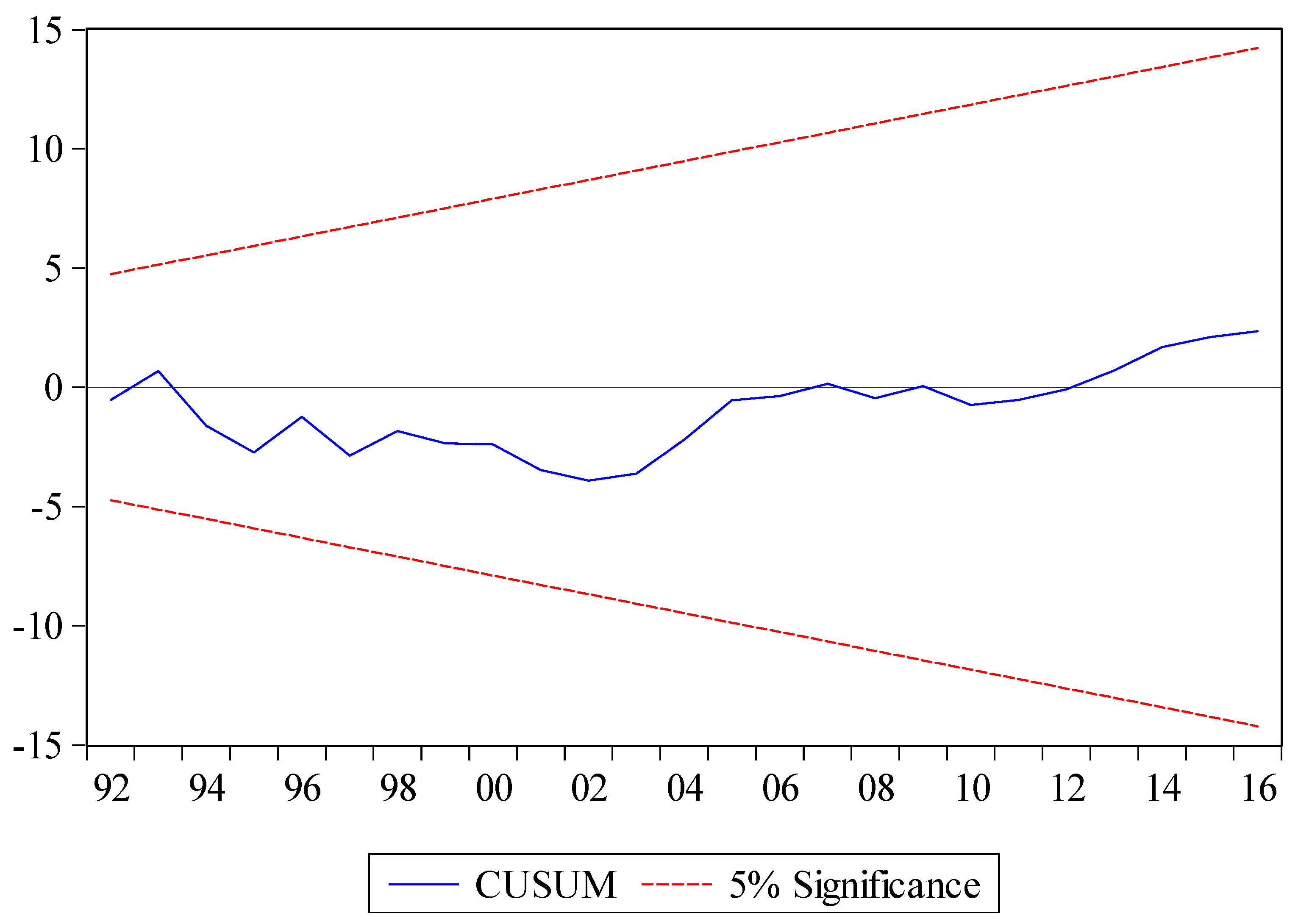
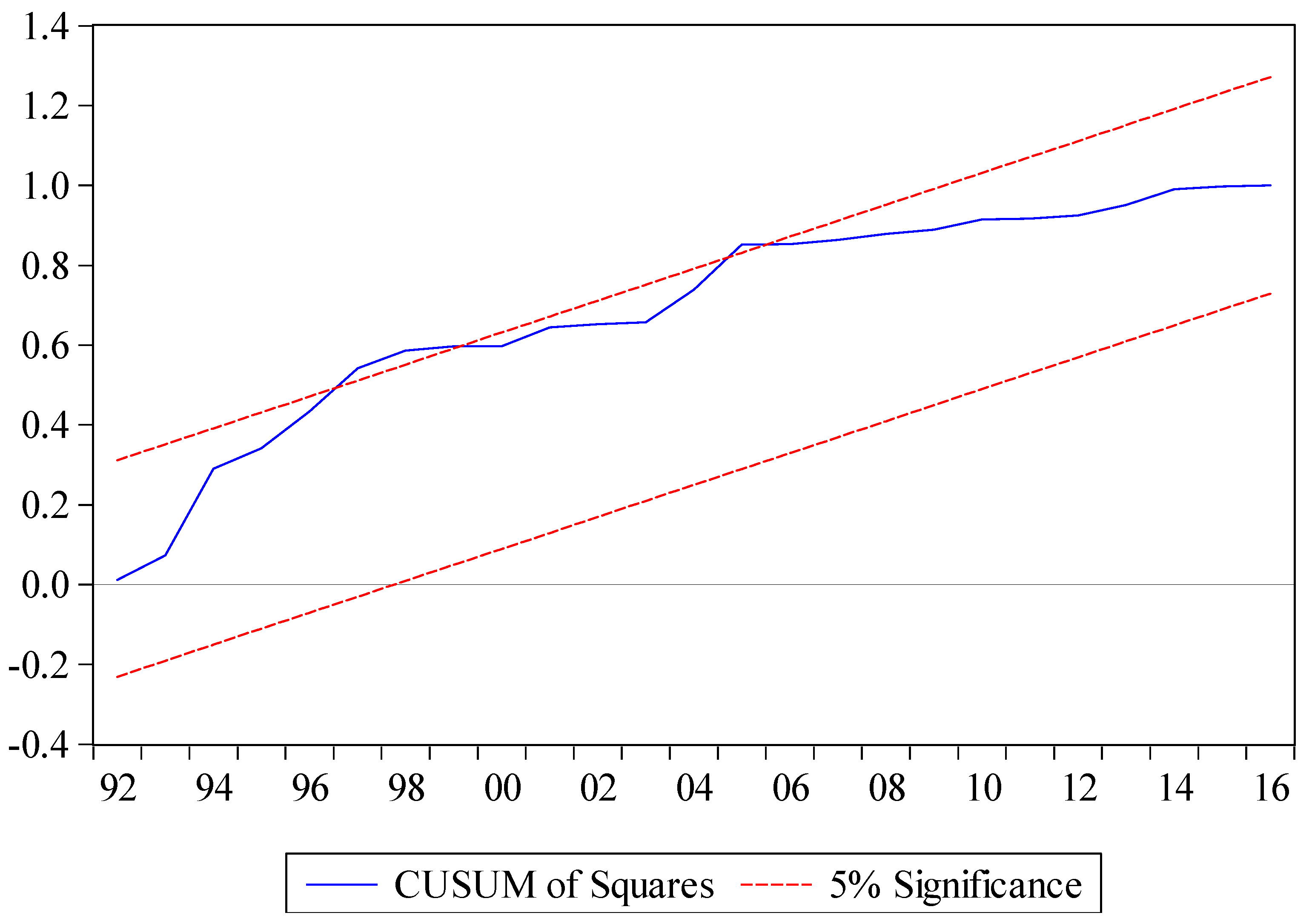
4.5. Diagnostic Tests

Table 8. Diagnostic checking of the ARDL model.

Test	F-Statistic	Prob.
Serial correlation	2.3505	0.1178
Heteroskedasticity	0.4290	0.5173

reports the consequences of diagnostic tests of the ARDL model. The estimated outcomes of the Breusch–Godfrey (BG) method verified that our ARDL model had no problem with serial correlation, while the results of the Breusch–Pagan–Godfrey (BFG) method verified that there was no problem of heteroskedasticity. Figure 1 and Figure 2 display the plots of the cumulative sum of recursive residuals (CUSUM) and the plot of cumulative sum of squares of recursive residuals (CUSUMS), which show that the ARDL model was stable over the sampled period.

4.6. VECM Results

The existence of co-integration offers an opportunity to evaluate a directional casual interconnection between study variables.

Table 9. VECM-based Ganger causality estimations.

Dependent	Independent Variables
Variable	ΔLNAP	ΔLNCR	ΔLNTR	ΔLNTW	ΔLNLF	ΔLNEC	ΔLNCO2
ΔLNAP	-----	6.9964 **	2.8847	4.4475	10.2873 ***	1.0093	1.7282
ΔLNCR	0.5306	-----	0.8025	1.6761	1.2048	0.1290	11.8917 ***
ΔLNTR	0.4467	2.0992	-----	0.2637	43.2285 ***	5.3851 *	6.0821 **
ΔLNTW	9.9108 ***	0.9168	1.2251	-----	5.6029 *	52.0655 ***	1.7066
ΔLNLF	0.2209	53.3740 ***	6.0783 **	4.8609 *	-----	1.6841	0.3188
ΔLNEC	0.6569	8.2059 **	2.9274	1.0222	2.1504	-----	0.5213
ΔLNCO2	2.5161	3.4813	5.2998 *	7.6488 **	2.8207	7.3640 **	-----

Note: ***, **, and * denote rejection of the null hypothesis at the 1%, 5%, and 10% levels, respectively.

demonstrates short-run causal links under the VECM, with essential implications for vigorous policy suggestions. Furthermore, the VECM approach established bi-directional and unidirectional associations between variables in the context of Pakistan. Considering the results of the two main variables, a unidirectional link was established from formal credit to agricultural production; from labor force to agricultural production; and from electricity consumption in the agriculture sector and tractors and tube wells to climate change (CO₂ emissions). In addition, there was a one-way causal link from CO₂ emissions to formal credit. The outcomes of additional variables show that labor force energy consumption and CO₂ emissions influence the quantity of tractors. Energy consumption, labor force, and agricultural production have a one-way link with tube wells. In return, credit, tractors, and tube wells have a significant link with labor. Finally, credit increases energy consumption in the short term in Pakistan.

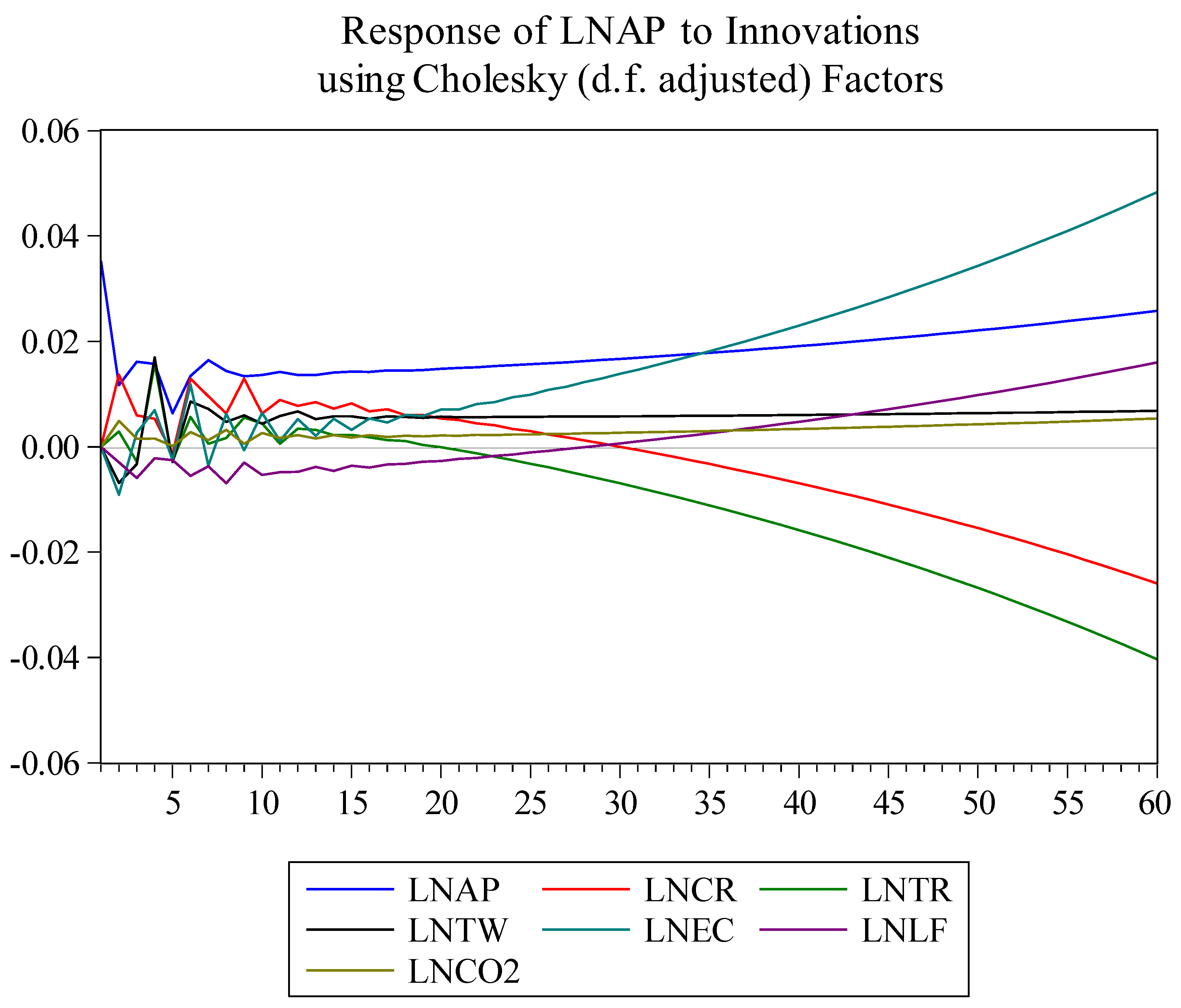
4.7. Impulse Response Function Results

The basic purpose of this approach is to check the evolution of variables in response to a shock to one or more variables in the model. This practice checks the behavior of variables at various periods and makes policy suggestions based on the responses of variables at different points of time. Using the data of 1983–2016, the impulse response function (IRF) under the VECM approach (shown in Figure 3), was twisted in nature from the first reply of the LNAP until the 23rd period. The first 26 periods had a smooth tendency for forecasting and regressing (except LNTW and LNEC), while trends varied for all variables from the 27th to the 60th period. Overall, the variations in response to shocks indicate that the connection of all variables was more significant in the long term than the short term. In the same line, the pattern of this relationship varied after 27 periods for most variables. Thus, the IRF validates the association of all variables with agricultural production, and indicates variations in this relationship that confirm the previous outcomes from the main models.

5. Conclusions and Policy Implications

The present study used the ARDL approach to assess the short- and long-run impacts of formal credit and climate change (CO₂ emissions) on agricultural production in Pakistan by means of additional variables such as technology factors (tractors and tube wells), labor force, and energy consumption within a multivariate framework from 1983 to 2016. In addition, this study also employed the VECM to determine the direction of causality among variables. The results of the ARDL bounds-testing approach confirm the presence of long-term cointegration relationships among formal credit, technology factors such as tractors and tube wells, energy consumption, labor force, CO₂ emissions and agricultural production over the study period. The consequences of long and short runs of the ARDL model revealed that formal credit, technology factors (tractors) and labor force positively and significantly affect agricultural production. This means that formal credit, technology use, and labor force are critical inputs in stimulating agricultural production. When we augmented the basic model by including CO₂ emissions as a climate change variable, results revealed that CO₂ emissions also positively affected agricultural production, while usage of tube wells and energy consumption had a negative impact on it in both the long and short term. Furthermore, the results of the VECM showed that a unidirectional relationship was established between formal credit to agricultural production; labor force to agricultural production; and electricity consumption and technology factors (tractors and tube wells) to climate change (CO2 emissions).

The role of formal credit is very much imperative as it is the key means of delivering several modern farming inputs with durable effects on agricultural production. As this empirical examination found that the use of agricultural technology like tractors play a dynamic role in increasing agricultural yield in a nation, our study therefore recommends that institutional sources of formal credit should be given to farmers in the form of special agricultural loans to buy modern agricultural technologies, with easy installments. Furthermore, the State Bank of Pakistan (SBP) must certify that formal organizations redeploy their lending instruments/services to those who claim them as prerequisite to achieving sustainable agricultural productivity, and they must develop an easy access to financial resources. Farmers will also need to become more pliable in order to capitalize on post-harvest advantages. Accordingly, the government should construct solid policies to overcome climatic change issues in the country.

Future studies should investigate the impacts of financial development and climate change (maximum and minimum temperatures, and precipitation) on major crop productivity by using country-level annual data, since the present study examined the impacts of formal credit and global climate change (CO₂ emissions) on agricultural production in Pakistan by using the ARDL model.

References

1. GOP. Pakistan Economic Survey 2018–2019; Economic Advisor’s Wing; Ministry of Finance, Government of Pakistan: Islamabad, Pakistan, 2019.
2. GOP. Pakistan Economic Survey 2017–2018; Economic Advisor’s Wing; Ministry of Finance, Government of Pakistan: Islamabad, Pakistan, 2018.
3. Chandio, A.A.; Jiang, Y.; Wei, F.; Guangshun, X. Effects of agricultural credit on wheat productivity of small farms in Sindh, Pakistan: Are short-term loans better? Agric. Financ. Rev. 2018, 78, 592–610. [Google Scholar] [CrossRef] [Green Version]
4. Hussain, A.; Thapa, G.B. Smallholders’ access to agricultural credit in Pakistan. Food Secur. 2012, 4, 73–85. [Google Scholar] [CrossRef]
5. Khan, R.E.A. Demand for Formal and Informal Credit in Agriculture: A Case Study of Cotton Growers in Bahawalpur. Interdiscip. J. Contemp. Res. Bus. 2011, 2, 10. [Google Scholar]
6. Akram, W.; Hussain, Z. Agricultural credit constraints and borrowing behavior of farmers in rural Punjab. Eur. J. Sci. Res. 2008, 23, 294–304. [Google Scholar]
7. Park, A.; Ren, C.; Wang, S. Microfinance, Poverty Alleviation, and Financial Reform in China. 2011. Available online: https://ora.ox.ac.uk/objects/uuid:e2e1e676-76d4-4dd1-96ab-c660a0c80eef (accessed on 17 June 2020).
8. Adejobi, O.; Atobatele, J. An analysis of loan delinquency among small scale farmers in Southwestern Nigeria: Application of logit and loan performance indices. East Afr. Agric. For. J. 2008, 74, 149–157. [Google Scholar]
9. Ahmad, A.; Jan, I.; Ullah, S.; Pervez, S. Impact of agricultural credit on wheat productivity in District Jhang, Pakistan. Sarhad J. Agric. 2015, 31, 65–69. [Google Scholar]
10. Ayaz, S.; Anwar, S.; Sial, M.H.; Hussain, Z. Role of agricultural credit on production efficiency of farming sector in Pakistan–a data envelopment analysis. Pak. J. Life Soc. Sci. 2011, 9, 38–44. [Google Scholar]
11. Bashir, M.K.; Gill, Z.A.; Hassan, S.; Adil, S.A.; Bakhsh, K. Impact of credit disbursed by commercial banks on the productivity of sugarcane in Faisalabad district. Pak. J. Agric. Sci. 2007, 44, 361–363. [Google Scholar]
12. Bashir, M.K.; Mehmood, Y. Institutional credit and rice productivity: A case study of District Lahore, Pakistan. China Agric. Econ. Rev. 2010, 2, 412–419. [Google Scholar] [CrossRef]
13. Akmal, N.; Rehman, B.; Ali, A.; Shah, H. The Impact of Agriculture Credit on Growth in Pakistan. Asian J. Agric. Rural Dev. 2012, 2, 579. [Google Scholar]
14. Iqbal, M.; Ahmad, M.; Abbas, K. The impact of institutional credit on agricultural production in Pakistan. Pak. Dev. Rev. 2003, 469–485. [Google Scholar] [CrossRef] [Green Version]
15. Sial, M.H.; Awan, M.S.; Waqas, M. Role of Institutional Credit on Agricultural Production: A Time Series Analysis of Pakistan. Int. J. Econ. Financ. 2011. [Google Scholar] [CrossRef] [Green Version]
16. Attiaoui, I.; Boufateh, T. Impacts of climate change on cereal farming in Tunisia: A panel ARDL–PMG approach. Environ. Sci. Pollut. Res. 2019, 26, 13334–13345. [Google Scholar] [CrossRef]
17. Chandio, A.A.; Ozturk, I.; Akram, W.; Ahmad, F.; Mirani, A.A. Empirical analysis of climate change factors affecting cereal yield: Evidence from Turkey. Environ. Sci. Pollut. Res. 2020, 27, 11944–11957. [Google Scholar] [CrossRef] [PubMed]
18. Guntukula, R. Assessing the impact of climate change on Indian agriculture: Evidence from major crop yields. J. Public Aff. 2019, 20, e2040. [Google Scholar] [CrossRef]
19. Dubey, S.K.; Sharma, D. Assessment of climate change impact on yield of major crops in the Banas River Basin, India. Sci. Total Environ. 2018, 635, 10–19. [Google Scholar] [CrossRef]
20. Praveen, B.; Sharma, P. A review of literature on climate change and its impacts on agriculture productivity. J. Public Aff. 2019, 19, e1960. [Google Scholar] [CrossRef]
21. Ali, S.; Liu, Y.; Ishaq, M.; Shah, T.; Ilyas, A.; Din, I.U. Climate change and its impact on the yield of major food crops: Evidence from Pakistan. Foods 2017, 6, 39. [Google Scholar] [CrossRef]
22. Ahsan, F.; Chandio, A.A.; Fang, W. Climate change impacts on cereal crops production in Pakistan. Int. J. Clim. Chang. Strateg. Manag. 2020. [Google Scholar] [CrossRef]
23. Abid, M.; Schneider, U.A.; Scheffran, J. Adaptation to climate change and its impacts on food productivity and crop income: Perspectives of farmers in rural Pakistan. J. Rural Stud. 2016, 47, 254–266. [Google Scholar] [CrossRef]
24. Chandio, A.A.; Magsi, H.; Ozturk, I. Examining the effects of climate change on rice production: Case study of Pakistan. Environ. Sci. Pollut. Res. 2020, 27, 7812–7822. [Google Scholar] [CrossRef]
25. Qureshi, M.I.; Awan, U.; Arshad, Z.; Rasli, A.M.; Zaman, K.; Khan, F. Dynamic linkages among energy consumption, air pollution, greenhouse gas emissions and agricultural production in Pakistan: Sustainable agriculture key to policy success. Nat. Hazards 2016, 84, 367–381. [Google Scholar] [CrossRef]
26. Abraham, T.W.; Fonta, W.M. Climate change and financing adaptation by farmers in northern Nigeria. Financ. Innov. 2018, 4, 11. [Google Scholar] [CrossRef]
27. Johansen, S.; Juselius, K. Maximum likelihood estimation and inference on cointegration—with applications to the demand for money. Oxf. Bull. Econ. Stat. 1990, 52, 169–210. [Google Scholar] [CrossRef]
28. Saqib, S.E.; Ahmad, M.M.; Panezai, S. Landholding size and farmers’ access to credit and its utilisation in Pakistan. Dev. Pract. 2016, 26, 1060–1071. [Google Scholar] [CrossRef]
29. Saqib, S.E.; Kuwornu, J.K.M.; Panezia, S.; Ali, U. Factors determining subsistence farmers’ access to agricultural credit in flood-prone areas of Pakistan. Kasetsart J. Soc. Sci. 2018, 39, 262–268. [Google Scholar] [CrossRef]
30. Carter, M.R. The impact of credit on peasant productivity and differentiation in Nicaragua. J. Dev. Econ. 1989, 31, 13–36. [Google Scholar] [CrossRef]
31. Chaudhry, M.G.; Hussain, Z. Mechanization and agricultural development in pakistan [with comments]. Pak. Dev. Rev. 1986, 25, 431–449. [Google Scholar] [CrossRef]
32. Feder, G.; Lau, L.J.; Lin, J.Y.; Luo, X. The relationship between credit and productivity in Chinese agriculture: A microeconomic model of disequilibrium. Am. J. Agric. Econ. 1990, 72, 1151–1157. [Google Scholar] [CrossRef]
33. Khandker, S.R.; Faruqee, R.R. The Impact of Farm Credit in Pakistan. Agric. Econ. 2003, 28, 197–213. [Google Scholar] [CrossRef]
34. Malik, S.L.; Broca, S.S.; Gill, M.A. Access by Farm Households to Credit from Formal Sources: The Case of Pakistan. Z. Ausl. Landwirtsch. 1996, 35, 269–280. [Google Scholar]
35. Saleem, M.A.; Jan, F.A. The Impact of Agricultural Credit on Agricultural Productivity in Dera Ismail Khan (District) Khyber Pakhtonkhawa Pakistan. Eur. J. Bus. Manag. 2011, 3, 38–44. [Google Scholar]
36. Shrestha, C.M. Institutional credit as a catalyst for agricultural sector growth: Evidence from Nepal. J. Econ. Dev. 1992, 17, 137–144. [Google Scholar]
37. Zuberi, H.A. Production function, institutional credit and agricultural development in Pakistan. Pak. Dev. Rev. 1989, 28, 43–55. [Google Scholar] [CrossRef] [Green Version]
38. Meyer, R.L. Analyzing the farm-level impact of agricultural credit: Discussion. Am. J. Agric. Econ. 1990, 72, 1158–1160. [Google Scholar] [CrossRef] [Green Version]
39. Agbodji, A.E.; Johnson, A.A. Agricultural Credit and Its Impact on the Productivity of Certain Cereals in Togo. Emerg. Mark. Financ. Trade 2019, 1–17. [Google Scholar] [CrossRef]
40. Afrin, S.; Haider, M.Z.; Islam, M. Impact of financial inclusion on technical efficiency of paddy farmers in Bangladesh. Agric. Financ. Rev. 2017, 77, 484–505. [Google Scholar] [CrossRef]
41. Malik, S.J.; Mushtaq, M.; Gill, M.A. The role of institutional credit in the agricultural development of Pakistan. Pak. Dev. Rev. 1991, 30, 1039–1048. [Google Scholar] [CrossRef] [Green Version]
42. Dong, F.; Lu, J.; Featherstone, A.M. Effects of credit constraints on household productivity in rural China. Agric. Financ. Rev. 2012, 72, 402–415. [Google Scholar] [CrossRef]
43. Obilor, S.I. The impact of commercial banks’ credit to agriculture on agricultural development in Nigeria: An econometric analysis. Int. J. Bus. Humanit. Technol. 2013, 3, 85–94. [Google Scholar]
44. Rahman, S.; Hussain, A.; Taqi, M. Impact of agricultural credit on agricultural productivity in Pakistan: An empirical analysis. Int. J. Adv. Res. Manag. Soc. Sci. 2014, 3, 125–139. [Google Scholar]
45. Rehman, A.; Chandio, A.A.; Hussain, I.; Jingdong, L. Fertilizer consumption, water availability and credit distribution: Major factors affecting agricultural productivity in Pakistan. J. Saudi Soc. Agric. Sci. 2019, 18, 269–274. [Google Scholar] [CrossRef]
46. Jan, I.; Manig, W. The Influence of Participation in Agricultural Support Services on Income from Agriculture: Results from the Multiple Regression Model (A Case from Rural Northwest Pakistan). Sarhad J. Agric. 2008, 24, 129. [Google Scholar]
47. Islam, M.T.; Nursey-Bray, M. Adaptation to climate change in agriculture in Bangladesh: The role of formal institutions. J. Environ. Manag. 2017, 200, 347–358. [Google Scholar] [CrossRef] [PubMed]
48. Zhou, L.; Turvey, C.G. Climate change, adaptation and China’s grain production. China Econ. Rev. 2014, 28, 72–89. [Google Scholar] [CrossRef]
49. Janjua, P.Z.; Samad, G.; Khan, N. Climate change and wheat production in Pakistan: An autoregressive distributed lag approach. NJAS-Wagening. J. Life Sci. 2014, 68, 13–19. [Google Scholar] [CrossRef] [Green Version]
50. Bank, W. World Bank (2016) World Development Indicators. 2016. Available online: http://data.worldbank.org/indicator (accessed on 30 December 2019).
51. Pesaran, M.H.; Shin, Y.; Smith, R.J. Bounds testing approaches to the analysis of level relationships. J. Appl. Econom. 2001, 16, 289–326. [Google Scholar] [CrossRef]
52. Engle, R.F.; Granger, C.W. Co-integration and error correction: Representation, estimation, and testing. Econom. J. Econom. Soc. 1987, 251–276. [Google Scholar] [CrossRef]
53. Ozturk, I.; Acaravci, A. Electricity consumption and real GDP causality nexus: Evidence from ARDL bounds testing approach for 11 MENA countries. Appl. Energy 2011, 88, 2885–2892. [Google Scholar] [CrossRef]
54. Dickey, D.A.; Fuller, W.A. Likelihood ratio statistics for autoregressive time series with a unit root. Econom. J. Econom. Soc. 1981, 49, 1057–1072. [Google Scholar] [CrossRef]
55. Phillips, P.C.; Perron, P. Testing for a unit root in time series regression. Biometrika 1988, 75, 335–346. [Google Scholar] [CrossRef]
56. Ng, S.; Perron, P. Lag length selection and the construction of unit root tests with good size and power. Econometrica 2001, 69, 1519–1554. [Google Scholar] [CrossRef] [Green Version]
57. Ahmad, N. Impact of Institutional Credit on Agricultural Output. Pak. Dev. Rev. 2011, 42, 469–485. [Google Scholar]
58. Hussain, A.H. Impact of Credit Disbursement, Area under Cultivation, Fertilizer Consumption and Water Availability on Rice Production in Pakistan (1988–2010). Sarhad J. Agric. 2012, 28, 95–101. [Google Scholar]
59. Javed, M.I.; Khurshid, W.; Hassan, I.; Ali, A.; Nadeem, N. Impact of institutional credit and extension services on productive efficiency of farms: Evidence from irrigated Punjab, Pakistan. J. Agric. Res. 2012, 50, 145–153. [Google Scholar]
60. Ahmad, D.; Chani, M.I.; Afzal, M. Impact of Formal Credit on Agricultural Output: Empirical Evidence from Pakistan. Sarhad J. Agric. 2018, 34. [Google Scholar] [CrossRef]
61. Zakaria, M.; Jun, W.; Khan, M.F. Impact of financial development on agricultural productivity in South Asia. Agric. Econ. Zemed. Ekon. 2019, 65, 232–239. [Google Scholar] [CrossRef] [Green Version]
62. Raifu, I.A.; Aminu, A. Financial development and agricultural performance in Nigeria: What role do institutions play? Agric. Financ. Rev. 2019, 80, 231–254. [Google Scholar] [CrossRef]
63. Longe, J. Economics of agricultural production in Nigeria. J. Policy Issues 2008, 1, 2–10. [Google Scholar]
64. Akbar, M.; Noor, F.; Ahmad, I.; Sattar, A. Impact of energy consumption and CO2 emissions on food production in Pakistan: An econometric analysis. Pak. J. Agric. Sci. 2018, 55, 455–461. [Google Scholar]
65. Chandio, A.A.; Jiang, Y.; Rehman, A.; Rauf, A. Short and long-run impacts of climate change on agriculture: An empirical evidence from China. Int. J. Clim. Chang. Strateg. Manag. 2020, 12, 201–221. [Google Scholar] [CrossRef]
Figure 1. CUSUM test.
Sustainability 12 05241 g001
Figure 2. CUSUM of squares test.
Sustainability 12 05241 g002
Figure 3. Impulse response function (IRF). Note: The obtained results from the impulse response function (IRF) for the VECM with regard to agricultural production (LNAP) in 60 future periods. LNCR = formal credit; LNLF = labor force; LNEC = consumption of electricity in agricultural sector; LNTR = tractors; LNTW = tube walls; and LNCO2 = carbon dioxide.
Sustainability 12 05241 g003