Neural Networks Applied to Microsimulation: A Prediction Model for Pedestrian Crossing Time

Abstract

Walking is the original form of transportation, and pedestrians have always made up a significant share of transportation system users. In contrast to motorized traffic, which has to move on precisely defined lanes and follow strict rules, pedestrian traffic is not heavily regulated. Moreover, pedestrians have specific characteristics—in terms of size and protection—which make them much more vulnerable than drivers. In addition, the difference in speed between pedestrians and motorized vehicles increases their vulnerability. All these characteristics, together with the large number of pedestrians on the road, lead to many safety problems that professionals have to deal with. One way to tackle them is to model pedestrian behavior using microsimulation tools. Of course, modeling also raises questions of reliability, and this is also the focus of this paper. The aim of the present research is to contribute to improving the reliability of microsimulation models for pedestrians by testing the possibility of applying neural networks in the model calibration process. Pedestrian behavior is culturally conditioned and the adaptation of the model to local specifics in the calibration process is a prerequisite for realistic modeling results. A neural network is formulated, trained and validated in order to link not-directly measurable model parameters to pedestrian crossing time, which is given as output by the microsimulation tool. The crossing time of pedestrians passing the road on a roundabout entry leg has been both simulated and calculated by the network, and the results were compared. A correlation of 94% was achieved after both training and validation steps. Finally, tests were performed to identify the main parameters that influence the estimated crossing time.

1. Introduction

In a world where urbanization is increasing—statistics predict a 58% growth in the world’s urban population by 2025 [1] and where all communities are tending towards more sustainable and environmentally friendly transport policies, it is understandable that pedestrians play a central role in the urban environment. Many transportation problems could be minimized and in some cases completely solved by proper planning of the urban environment: The development of walkable spaces could reduce the problems of congestion in city centers and pollution could decrease if people prefer to walk rather than using other means of transport. Of course, walking should be encouraged, and this is closely linked to the level of safety guaranteed by the available infrastructures.

A well-known and sophisticated tool for planning and design of transportation infrastructures is microsimulation. This technique is already widely used in transportation engineering and has many advantages; in particular it provides the possibility of studying various infrastructural options without actually realizing them, in order to better meet the needs of the considered road users, may they be Levels Of Service (LOS), emergency needs or safety-related issues. Certainly, to be useful, it is necessary to verify the accuracy and reliability of the developed models and the obtained results have to be checked: calibration and validation steps are necessary to be run, processes that request a long elaboration period and several efforts [2,3].

Many methods and techniques have been applied to calibrate traffic microsimulation models: trial-and-error procedures [4,5], statistical methods [6,7,8] and evolutionary algorithms [9,10,11]. One of the most commonly used methods for the calibration of traffic microsimulation models is the Genetic Algorithm (GA), a stochastic based search method, which is based on the concept of biological evolution [11,12,13].

This paper focuses on improving the reliability of a microsimulation tool for modeling pedestrian behavior by applying Neural Networks (NN).

Previous research developed by the research team on the investigation and modeling of motorized traffic [14,15,16] has shown that neural networks provide a good response, when applied to vehicular traffic issues. These studies [14,15,16] demonstrated that the formulated neural network, despite giving a good prediction of travel time, did not have similarly successful responses for vehicle queue parameters. Once calibrated via neural network applications, the microsimulation model provided vehicle queue parameter values that differed by less than 5% from the measured ones.

The aim of this paper is to investigate the possibility of applying neural networks in the calibration of a microsimulation model of pedestrian movements. Pedestrian behavior has its own specifics and is influenced by the cultural milieu perhaps more than vehicular movement [1,17,18,19]. Also, the pedestrian population includes all vulnerable groups, from children at the beginning of their independent movement, to elderly pedestrians with mobility difficulties as well as pedestrians with various disabilities (motor disabilities, low vision, etc.) [18]. Given the greater dispersion of reaction times and velocities of the pedestrian population in comparison to the driving population, the question of the possibility of predicting the crossing time in the conflict zone becomes critical for model calibration [19,20,21]. Also, although walking is part of the transport system, having its own particular behavioral rules and characteristics, it cannot be simulated by the behavioral model normally used for cars. The aim of the present work is to obtain a reliable model to predict one aspect of the simulated pedestrian behavior. The developed procedure is the first contribution to the development of a calibration methodology, whose final goal is to fine-tune non-directly measurable modeling parameters on the basis of a model output that is characterized by its easy measurability. For this purpose—based on previous experience—neural networks were selected as a possible applicative tool. The selected neural network will be trained, validated and evaluated in order to create a predictive model of pedestrian simulated behavior at a specific location type. Crossing times of pedestrians walking on a zebra crossing at a roundabout entry leg will be both simulated and calculated by the network and results compared. Tests are also developed to underline which input parameters have the greatest influence on the selected output. Herein, a limitation of the research presented in this paper should be pointed out: since it deals with the formulation of the model to predict the micro-simulated behavior of pedestrians, representing the first important step towards the development of the whole calibration methodology, the calibration of the initial model parameters cannot be worked out. Of course, a check of the validity of the developed microsimulation model was carried out, in order to understand if it reproduced a realistic behavior. Nevertheless, a precise calibration of the model needs its parameters to be fixed. To train the neural network, it is necessary to create a huge number of combinations of the model’s parameters—which are each time different, in order to make the neural network learn the relationship between these parameters and the selected output. Only at the end of the whole calibration process is it possible to apply the selected, trained neural network to obtain the combination of input parameters which, put in the microsimulation model, gives the best output, i.e., the crossing time which is the most similar to the real, measured crossing time.

The aim of the paper is to highlight the effective possibility of applying neural networks in the process of calibration, by showing that the selected, trained network is able to reproduce the model’s outcomes. This step is central, because if the neural network can reproduce the microsimulation output, then it can be used to calibrate the model. The calibrated model will be the outcome of the whole, further research.

The paper is structured as follows: the next section explains the 5-step-methodology used in the research: the location and period for video footage recording are described; the model set up, the peculiarities of both the zone and the behavior of traffic participants and the way they were tackled in the model are presented; after this, an overview of the equation and parameters governing the micro-simulation model is given and the choice and preparation of parameters is illustrated. Finally, the formulation of the neural network architecture is characterized. Section 4 presents the results provided by the neural network, describing the measures of performance used for the evaluation, the results of the training step and the ones achieved after the validation of the prediction model. In the end, Section 5 deals with conclusions and future research.

2. Related Works

In this section, a literature review about the main applications of neural networks to pedestrian questions will be provided. In addition, a brief overview of the main tools applied to microsimulation model calibration is worked out.

2.1. Use of Neural Networks in Pedestrian Research

In the pedestrian study area, neural network practice is mainly limited to the progression of detection approaches.

In [22], authors deal with pedestrian detection and classification. They use various methods for feature extraction and classification, among which there are also neural networks. NN are used in both steps: firstly, as one of the methods to be compared, in the second one to develop the training of the recalled techniques. As feature extraction method, they use a feed-forward neural network with local receptive fields. This seemed to achieve the best results among all the techniques involved.

The authors of [23] develop a pedestrian counting technique, starting from the data obtained by a single camera. The peculiarities of the system are the use of feature histograms and the feature normalization. It is interesting to notice that the authors try two kinds of supervised training: one using linear fitting and the other utilizing neural networks and show that neural networks have better performance compared to linear fitting.

In [24], the studiers develop a pedestrian detection method based on convolutional neural networks, seeming to outperform traditional detection techniques. Specifically, they applied two state-of-the-art neural networks—AlexNet and GoogLeNet—to the problem of pedestrian detection and evaluate their results following the Caltech Pedestrian Detection evaluation protocol.

The authors of [25] developed a Deep Learning Algorithm to be applied to Advanced Driver Assistance Systems for the observation and detection of pedestrians, by fusing SqueezeNet and the YOLO detection network. Their findings show both high accuracy and robustness, and they propose the possibility of implementing the algorithm both on mobile phones and on embedded systems. Also, the authors suggest reducing the number of parameters of the neural network in order to obtain a faster algorithm with a still acceptable level of accuracy. Also, [26] deals with pedestrian detection. In this research, the authors address a Fused Deep Neural Network (F-DNN) to achieve faster and more accurate detection. By testing the proposed algorithm on different scenarios, the authors highlights its better performance in terms of both robustness and speed in comparison to the other state-of-the-art models. The work [27] formulates a Support Vector Machine (SVM) model to use the micro Doppler features of radar signals to distinguish objects from people around vehicles and, in this way, to detect near crash situations involving pedestrians. The aim of the article is to improve—by applying SVM—both the classification performance and speed, and it reached a 0.12 m/s velocity resolution. Among all the evaluated approaches, the performance was obtained by a polynomial kernel approach, which obtained a 99.5% accuracy rate and a processing time of 0.073 s. The authors of [28] deal with Deformable Part Models (in the following DPMs) and convolutional neural networks (CNN). In particular, the authors developed a new model, describing DPMs as a composition of 2 CNNs. The model they achieved is called Deep Pyramid DPM and it is constituted by two neural networks. As the input, it takes an image pyramid, as the output it performs a pyramid of object detection scores.

Also, face detection has been worked out thanks to neural networks. Specifically, in [29], a hybrid neural network method for real-time detection of faces made up of local image sampling, SOM neural network and a CNN is developed and applied to a database of 400 images of 40 individuals characterized by different poses, facial details and expressions. In [30], a system to detect not only walking pedestrians, but also standing people, is carried out thanks to the use of neural networks. In [31], the authors introduce a deep neural network with a star topology. The goal of the network is to predict pedestrian trajectories. To reach it, a hub network is formulated to produce a comprehensive representation of the crowd, while host networks predict the future trajectories of each pedestrian. The proposed architecture was evaluated on two datasets where different interactions happen: specifically, walking side by side, collision avoidance and direction changing are among the considered behaviors. Results were compared in terms of Average Displacements Error and Final Displacement Error with three state-of-the-art models: Social LSTM, Social GAN and Social Attention. Regarding the accuracy rate, the StarNet architecture outperformed all the other models, while in terms of computational time cost, it was second only to the LSTM model.

Finally, in [31] a back propagation—Ward net—is formulated to predict children’ reaction time at signalized intersections. The structure of the network is characterized by five layers: one input layer, three hidden layers and one output slab. In the input layer there are seven inputs—age, gender, children with special needs, movement in group, adult supervision, mobile phone texting activities and mobile phone listening—while each hidden slab has five neurons, and the output layer contains one output neuron.

The results show a 94.56% of correlation and a mean absolute error of the prediction equal to 0.348 s.

2.2. Algorithms Applied to Calibration of Pedestrian Microsimulation Models

In the field of pedestrian microsimulation, an important point is model assessment. To reach it, various calibration methodologies were developed and can be found in the literature. Mainly, three main tools are addressed: maximum likelihood estimation (MLE), genetic algorithm (GA) and artificial neural networks (ANN).

In [32], a MLE methodology was applied to the calibration of the microsimulation tool NOMAD for evacuation conditions. Using as inputs trajectory data divided for three age classes—children, adults and the elderly—the authors focus on the tuning of four elements, which are the acceleration time, free speed, an interaction term identified as acceleration and the interaction distance.

The authors of [12] implement a genetic algorithm to estimate the values of parameters A and B, i.e., the strength and range of interaction between agent-agent and agent-obstacle, of a social force inspired model, applied to pedestrian flow at a metro entrance. Though many results are reported in this research, direct metrics—like the RMSE—are not summarized, meaning an assessment in relation to other works is difficult.

An interesting comparison among different calibration methodologies is worked out in [33]. The researchers apply the MLE, Nelder-Mead optimization algorithm and Genetic Algorithm on common simulated data to calibrate parameters A and B—strength and range of interaction among pedestrians—to be able to test and compare them. As result, they determined that the Genetic Algorithm has to be preferred over the other techniques, while MLE is not recommended.

Artificial Neural Networks (ANN) are introduced in [34] for pedestrian microscopic model calibration. In this paper, ANNs are compared to multiple linear regression (MLR) for the prediction of pedestrian gap acceptance. The comparison made considering RMSE, MAPE, correlation coefficient and R² shows that ANN performs much better than MLR for RMSE and MAPE, and is comparable to regarding the correlation coefficient and R².

Briefly enlarging the review to transportation research, the same three main methods are highlighted [6,15,35]. Specifically, regarding neural networks, [14,15,16] found that neural networks are able to reliably predict time variables, such as travel time and crossing time, and a procedure was developed to calibrate traffic microsimulation models. Also in [35], where a review of the applications of neural networks in transportation research is worked out, it is underlined that neural networks are more effective in estimating travel times than other methods. In [36], when comparing and contrasting statistics and neural networks, authors emphasize various advantages of applying neural networks: they underline the efficiency of this tool in terms of accuracy and development time, their flexibility as well as the opportunity of applying few restrictions in comparison to statistics, where many hypotheses and assumptions are to be taken. All these observations, as well as the applications of neural networks to other parameter estimation issues, put the basis for the use of this tool in the present research. Moreover, the effectiveness of neural networks in predicting time variables, which emerged from previous authors’ research [14,15,16], and the convenience of use when input parameters that need to be tuned are not directly measurable [14,15,16], justify their choice in a noteworthy way.

3. Method

The general method used to formulate and evaluate the neural network consists of 5 main steps (Figure 1).

First, real data were obtained to adapt the model both geometrically and in terms of flow to the real chosen situation and to compare—in further evaluations—the simulated outputs with the real values of the chosen parameter. With this information, the microsimulation model was created and visually tested to avoid unrealistic behavior.

The second step involved the selection of suitable parameters, which mainly influence pedestrian behavior, but also consider the interaction with motorized road users and are to be used as inputs for the neural network. Then the most suitable microsimulation output was selected, which should also be used as an output of the neural network. After these selections, a database with random input combinations was generated. Each of these combinations was linked by simulation to a corresponding output value. The third step consisted in the formulation of the neural network and its training. The results of this step were evaluated in relation to the criterion of learning outcomes.

Finally, a new data set was used to evaluate the network, taking into account the criterion of generalization. In the next paragraphs, the steps are described in detail.

3.1. Data Gathering

As a starting point for the model setting up and the development of the neural network, a real situation had to be selected.

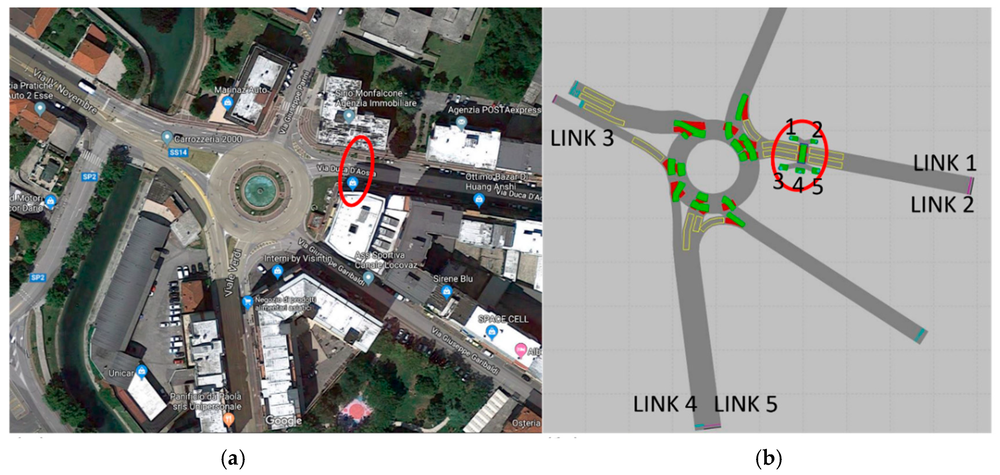
It was decided to record an unsignalized pedestrian crossing, which is located on the entry leg of a roundabout: the considered infrastructure is located in Monfalcone (GO), a city in the Italian region Friuli-Venezia-Giulia. The roundabout is located in the urban area of the municipality and connects the city center with the main neighboring towns. The crossing passes two unidirectional lanes of the same roundabout entry leg and connects pubs and cafés with offices, schools and shops. Both pedestrian movements and conflicting vehicle traffic were recorded for a whole week, during the two peak hours of the city, i.e., from 7.30 to 9.30 a.m., obtaining more than 1000 recorded pedestrians.

The recordings were analyzed using a semi-automatic software that allows selected detections to be automatically saved and the users involved to be tracked manually. This step made it possible to obtain a huge amount of data on both motorized and non-motorized users. Due to the research objective, the selected real-world data, which were then used in the model, were pedestrian speed distribution, pedestrian flow and its split rate, vehicular flow and speed (

Table 1. Real-world data implemented in the microsimulation model.

Pedestrian Speed Distribution	Lower Bound	3.12	km/h
	Upper Bound	8.71	km/h
pedestrian flows (from-to)	1–3	43	peds/hr
	2–4	20	peds/hr
	3–5	3	peds/hr
	4–1	46	peds/hr
	5–2	20	peds/hr
vehicular flows (on link)	2	325	veh/hr
	1	325	veh/hr
	3	650	veh/hr
	4	165	veh/hr
	5	165	veh/hr
vehicular speed distribution	lower bound	15.5	km/h
	upper bound	50.67	km/h

). In Table 1, the numbers reported in the second column, which refer to pedestrian flows, represent the start and end zones of the pedestrian trip, the ones referring to vehicular flows indicate the link on which vehicles travel (see Figure 2).

Geometrical data have also been collected and they have been gathered directly from official map information, provided by the municipality.

3.2. Micro-simulation Model Set Up

The model, on which neural networks were trained, was developed with the commercial microsimulation software Vissim. The simulated geometry and the allowed manoeuvers are exactly the same as the real ones (Figure 2;

Table 2. Geometrical data of the road intersection.

Geometrical Data
Crossing length	10.25	m
Crossing width	4	m
Entry leg width—before crossing	11.65	m
Entry leg width—after crossing	7.65	m
Entry lane width—before crossing	5.95	m
Entry lane width—after crossing	3.95	m
Number of lanes	2
Entry lane curvature	34.58	m
Distance of the crossing from yielding line	20.34	m
Length of the curved part	29.57	m
Distance of the crossing from the beginning of the curved part	5.23	m
Ring internal radius	13	m
Ring external radius	22	m
Number of lanes on the ring	2
Ring lane width	4.3	m

).

In order to obtain a realistic simulation, vehicular traffic was regulated according to the Wiedemann 74 behavior, which is the suggested behavior for urban traffic modeling [37], while pedestrian traffic was regulated according to the social force model, which was implemented thanks to the Viswalk add-on.

Four main problems were encountered in the reproduction of the site: The first concerned the network geometry and in particular the need to model the entire roundabout or just the recalled entry leg. The decision was made to model the entire roundabout and its oncoming and outgoing legs, as the facility is very crowded and each incoming and outgoing flow is affected by the others. The second question was related to the path of modeling pedestrian movements. In fact, simulated pedestrians can move on a “pedestrian area” or on a “link used as pedestrian area”. After heuristically implementing both possibilities and critically observing the reproduced behavior, it was decided to use the “link used as pedestrian area”, since it visually provided the response best fitting real observations. Finally, the third question concerned vehicular behavior: Italian drivers do not usually stop at pedestrian crossings unless they consider it necessary. This led to the need to realistically reproduce this type of yielding behavior. To solve the problem, priority rules and speed reduction areas were jointly used. The first ones let the pedestrian be yielded by the oncoming vehicles, while there were 4 “speed reduction areas” placed, 2 in proximity of the crossing and 2 just before the stop line to enter the roundabout circle, to allow vehicles to reduce their speed, thus well simulating the real observed outcomes.

A fourth complication was set by pedestrian generation: in the selected scenario, pedestrians can arrive from 5 different directions—3 on the left and 2 on the right side—and they can reach 5 different destinations. To solve this problem, a pedestrian area and the corresponding pedestrian input for each of the listed directions were created.

Summing up, the network geometry consists of 49 links: 16 vehicular links defining the oncoming and outgoing roads and the roundabout circle lanes, 12 links used as pedestrian areas and 5 pedestrian areas and 12 connectors.

3.3. Parameter Choice and Preparation

To successfully formulate and train a neural network, the parameter choice, on which the selected network will work, is of primary importance. Since the aim of the research is to assess pedestrian crossing behavior in an environment where the interaction with vehicular flow is not uninfluential, it was decided to work both on pedestrian and vehicular behavioral parameters. Specifically, a total of 8 parameters were selected, 5 of which relate to pedestrians and 3 of them linked to vehicular traffic. Pedestrian movement was modeled thanks to the Social Force Model (SFM) [38]. As stated in [39], on the one hand, this model is easy to understand, but on the other hand, it is difficult to interpret and measure the parameters from which it is composed, which strongly influence diverse behavioral aspects.

The basic concept of the SFM is that each pedestrian, defined by its desired speed and target time, moves towards its destination ruled by the so-called social forces [38]. These effects are: the attractive forces that lead each pedestrian to its destination $F_{\alpha }^0$; the repulsive forces among pedestrians and among the individual and obstacles and the attractive forces due to other pedestrians/objects [38]. In Vissim/Viswalk, the Social Force Model expression (Equation (1)) is adapted and some parameters governing the equations, emerge:

$$\mathrm{F}={\mathrm{A}}_{{\mathrm{soc}}_{\mathrm{isotropic}}}\mathsf{\omega }\left(\mathsf{\lambda }\right)\exp \left(-\frac{\mathrm{d}}{{\mathrm{B}}_{{\mathrm{soc}}_{\mathrm{isotropic}}}}\right)\mathrm{n}+{\mathrm{A}}_{{\mathrm{soc}}_{\mathrm{mean}}}\exp \left(-\frac{\mathrm{d}}{{\mathrm{B}}_{{\mathrm{soc}}_{\mathrm{mean}}}}\right)\mathrm{n}.$$

(1)

In detail, these are the following:

$\mathsf{\omega }\left(\mathsf{\lambda }\right)$ is a parameter depending on lambda calculated for each physical force opposing the main force F [37].

d is a parameter dependent on a further formulation, which indicates the distance between two pedestrians [37].

n is the vector pointing the influenced pedestrian to the influencing one [37].

Tau (τ): relaxation time as expressed in Helbing’s original model. It relates the difference between the desired speed and direction to the current speed and direction. Though it is not directly present in Equation (1), it is used to express the force leading the pedestrians to its destination [37].

Lambda_mean (λ): amount of anisotropy. It regulates the effect of phenomena that take place in the back of the considered pedestrian [37].

A_soc_isotropic and B_soc_isotropic: non-measurable parameters that control the two forces among pedestrians [37].

A_soc_mean and B_soc_mean: respectively define the strength and typical range of the social force between pedestrians [37].

Also, other parameters influence pedestrian movement in the Vissim/Viswalk simulation tool, and should be considered. These are:

Noise: introduces the random forces, which are systematically added to the calculated forces [37].

React_to_n: the number of pedestrians considered for the calculation of the forces [37].

Side_preference: defines whether opposing pedestrians prefer using the right or left hand side when passing each other [37].

Queue_order and Queue_straightness: specify the properties of the queue [37].

In the calibration attempt developed in [40], the authors give an insight into which modifications are brought about by the change of some of the recalled parameters (

Table 3. Vissim (i.e., the applied micro-simulation software) parameters and their modifications as proposed by Kretz [41].

Parameters	Initial Parameter Values	2nd Parameter Set Values	3rd Parameter Set Values	Unit of Measurement
Radius of pedestrians	15			10−2 m
A social_mean	0.5	0.1	2.5	m/s²
B social_mean	2.8			m
B physical, border	100			1/s2
A social, isotropic	25	10	100	m/s²
B social, isotropic	0.2	0.05	0.3	m
τ	0.4			s
Friction force	0
Side preference	Right
Velocity dependence VD	2			s
λ	0.1
Longitudinal scale	0.25
maximum n pedestrians	5	15	15

). In Table 3, additional parameters to the ones reported in Equation (1) are also considered. They are: the radius of pedestrians, which indicates the size of the bidimensional ellipse containing the shape of a pedestrian [40]; B physical, a border that is a theoretical parameter controlling the force between a pedestrian and the border of a location [40]; friction force, a component of the main force F, together with attractive and repulsive forces; VD is a theoretical parameter of Vissim namely “velocity dependence”, which is expressed in terms of seconds and which involves various other parameters, nevertheless it is not exactly defined in [37]; velocity is the speed of pedestrians; longitudinal scale is a dimensional parameter of the model; maximum number of pedestrians represents the maximum number of interacting agents considered in the simulation.

A literature review has been developed focusing on parameter fine-tuning and, from these findings [37,39,40,41], 5 pedestrian parameters—tau, lambda, Asoc_iso, Bsoc_iso, side_pref—and their ranges have been outlined in

Table 4. Selected pedestrian and vehicular input parameters for the neural network.

Input	Name	Min	Max
I1	Tau	0.05	2
I2	Lambda	0	0.4
I3	Asoc_isotropic	3	7
I4	Bsoc_isotropic	0.1	10
I5	Side_preference	−1	1
I6	Average standstill distance	1	3
I7	Additive part of safety distance	1	5
I8	Multiplicative part of safety distance	1	6

.

Since in the considered situation the interaction with vehicular flow is strict, vehicular parameters also have to be considered. In particular, the model governing vehicular behavior is Wiedemann 74, and the selected parameters to be used are the three that most affect the car-following model, i.e., average standstill distance, defining the mean desired distance between two cars, the additive part of safety distance and multiplicative part of safety distance, which are values used for the calculation of the desired safety distance [37].

Geometric characteristics and traffic load are also very important parameters, but they are entered as inputs to the model for each location separately. In Table 4, vehicular parameters and their ranges are also summarized.

The selection of a feasible output is also important. For this study, pedestrian crossing time has been chosen as assessment output for the neural network, because of its ease to be measured both from footage (semi-automatically as well as manually) and microsimulation results.

After parameter choices, these have to be stored in a suitable way to be read as input values by the neural network. The requirements needed in order to obtain a good training of the network are the amount of data, their randomness and a good quantity of repetitions of each combination.

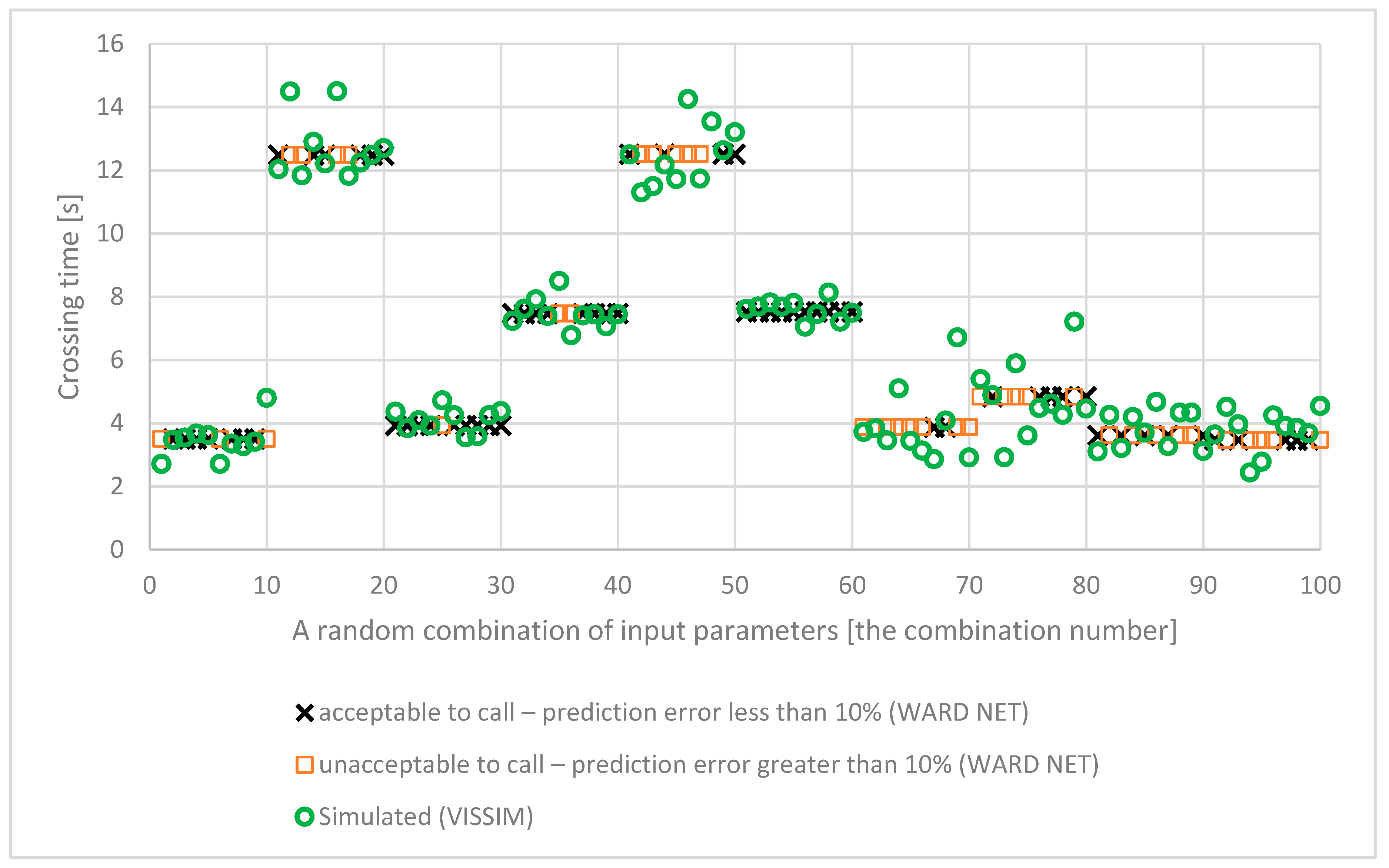
For this study, a database of 100 random combinations of input-output values was worked out in Excel. Each combination is made up of a random selected value for each one of the 8 input parameters with a step of 0,1 and the resulting crossing time obtained by implementing the chosen input combination in the Vissim model. Also, parameters were selected in such a way that their ranges are comprised in the same magnitude unit, in order to avoid great range differences. To have a sufficient number of repetitions, ten simulations have been run for each random combination with an initial seed random value of 42 and an increment of 10 and a simulation of 1 timestep/second. In this way, we ensured that the same ten possible traffic scenarios were analyzed for each combination of input parameters. The number of simulations has been chosen as a compromise to the pseudo-stochastic working method of the model: as a matter of fact, it simulates a phenomenon which has a stochastic nature—traffic flow—but at the same time the experiment has to be repeatable, which means that the same “random seed” parameter value (random number generator) gives the same output.

Here the mean output value of ten simulations was used as the final output of the simulation for each random combination of selected input parameters.

Following the most used protocol [42] of the created dataset, 80% has been used for the training of the network, while the remaining 20% has been utilized as a test bed for the first evaluations (test and validation).

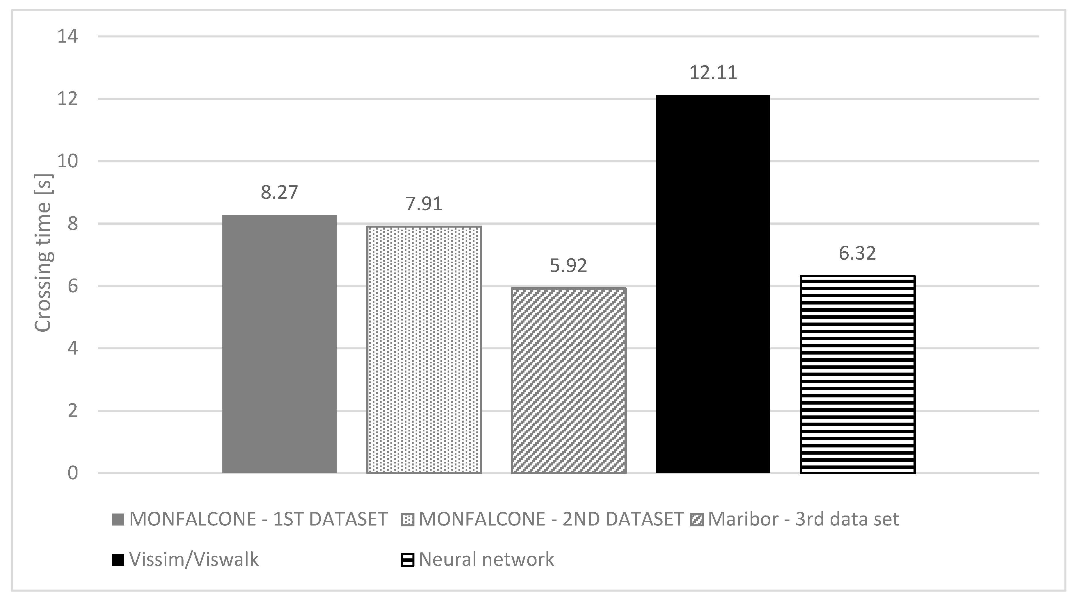
An additional database corresponding to the 20% of the initial one was generated after network training and testing. This completely independent database, which did not participate in either the training set or the test set in the neural network learning process, served to independently confirm the ability to generalize the selected neural network. Indeed, the goal of training a neural network is to achieve a good generalization, being able to be applied to much larger databases than the one on which it was trained. In the specific case, the neural network trained on a database of 100 combinations, will be applied to 3–4 times larger databases, which compare crossing times measured in real traffic conditions and crossing times as obtained by microsimulations using the neural network prediction function implemented in the calibration process for different values of input parameters.

3.4. Comparison between Measured and Simulated Pedestrian Crossing Time

By using default parameters in the microsimulation model, an average crossing time of 12.11 s has been obtained. This value appears to be higher than the crossing time measured in situ, whose mean equals 8.27 s.

Table 5. Comparison between the crossing time obtained with the microsimulation model and the one measured in situ.

	Simulated Crossing Time [s]	Real-World Crossing Time [s]
Mean	12.11	8.27
Standard error	0.56	0.13
Median	11.0	8.0
Standard deviation	6	1.54
Asymmetry	1.18	0.73
Min	4	4
Max	35	14
Confidence level (95.0%)	1.1	0.26

summarizes the descriptive statistics for the crossing time.

The simulated crossing time is 3.84 s higher (46.4%) than the measured one, justifying the need for a calibration process to be worked out.

In the following, the formulation of a neural network is presented, which—through its prediction function—could be used in a calibration program procedure. The aim of this paper is to show the applicability of the neural network to the prediction of the microsimulation output, giving the opportunity to effectively use it in the calibration process under development. The goal of the neural network, therefore, is not to outperform the Vissim/Viswalk microsimulation software; rather, it is to learn the relationship between the selected microsimulation input parameters and the simulated output, the crossing time.

3.5. Neural Network Formulation

Previous works [14,15] about the calibration of vehicular traffic models have considered the application of various kinds of neural networks and their performance, examining 176 neural network configurations. On the basis of these considerations and of previous experiences, for the present issue, a ward network was implemented in the Neuroshell2 program.

Ward nets, better known as feedforward networks, are neural networks structured in such a way that the neurons of a layer have the outputs of the neurons in the precedent slab as input signals [43]. A feedforward network, in which each neuron of one layer is linked to the ones of the adjacent layer, is called fully connected [43]. An example of a fully connected feedforward network can be seen in Figure 3.

The adopted neural network is made up of 5 layers: the input layer has 8 neurons, corresponding to the 8 selected input parameters, the output slab has one neuron, i.e., the selected output parameter—pedestrian crossing time, while layers 2, 3 and 4 are hidden layers and each one is composed of 4 hidden neurons.

The architecture of the neural network has been chosen following some of the rules found in literature [43,44,45] and the knowledge acquired by previous experiences [16]. The number of input and output neurons is related to the number of initial parameters to be used and desired outputs to be evaluated. The selection of the number of hidden neurons is more complicated and has important consequences for the results of the network: indeed, as reported in [46], too many hidden neurons can cause over-fitting issues and degrade the generalization ability of the neural network. Much research exists on methods to select the best number of hidden neurons [44,46]: following [47]’s indications, a correct number of hidden neurons can be suggested by applying the formula (Equation (2))

$$\frac{{\mathrm{n}}_{\mathrm{in}}+{\mathrm{n}}_{\mathrm{out}}-1}{2}$$

(2)

where ${\mathrm{n}}_{\mathrm{i}\mathrm{n}}$ represents the number of input neurons and ${\mathrm{n}}_{\mathrm{o}\mathrm{u}\mathrm{t}}$ is the number of output neurons. Also, a general rule of thumb is to select a number of hidden neurons belonging to the interval between the number of inputs and outputs.

Considering these two rules, 4 neurons have been chosen for the hidden layers of the network.

Regarding the number of hidden layers, initially it was selected according to the literature [45,46,47] and empirically, on the basis of previous experiences [15,16], then 10 different configurations were tested and the one giving the best results was chosen. As with any optimization procedure, the question arises whether the selected network architecture is a local or global optimum. Given the learning outcomes and their practical application, this question was not focus of our further research.

The main feature of the selected network stands in the activation functions. As a matter of fact, the input layer is connected to the hidden ones by the same linear function, but each hidden layer is linked to the output slab through a different activation function in

Table 6. Features of the chosen neural network—in terms of layers, neurons, activation function, learning rate, momentum and initial weight.

Layers	Neurons	Activation Function	Learning Rate	Momentum	Initial Weight
1 (input)	8	Linear [−1,1]	0.1	0.1	0.3
2 (hidden)	4	Gaussian	0.1	0.1	0.3
3 (hidden)	4	Tanh	0.1	0.1	0.3
4 (hidden)	4	Gaussian compact	0.1	0.1	0.3
5 (output)	1	Logistic	0.1	0.1	0.3

.

In Figure 4, the neural network architecture is outlined.

4. Results and Discussion

In this section, the results of the formulated neural network are presented and evaluated. The first paragraph reports the ward network’s results, the related performance measures and the analysis of input parameters; the second paragraph sums up the results of the validation of the neural network.

4.1. Neural Network Results and Analysis of Input Parameters

In the following, the best result provided on a test data set is reported, on which the ability to generalize the network was initially evaluated. The selected neural network showed a very good correlation with the initial data; as can be inferred from the statistics reported in

Table 7. Statistical results of the formulated neural network.

Performance Metrics for the Evaluation of the Formulated Neural Network
R squared	0.9509	Correlation coefficient r	0.9755
r squared	0.9516	Percentage within 5%	38.000
Mean Squared Error	0.595	Percentage within 5% to 10%	21.000
Mean Absolute Error	0.559	Percentage within 10% to 20%	25.000
Min. Absolute Error	0.007	Percentage within 20% to 30%	9.000
Max. Absolute Error	2.837	Percentage over 30%	7.000

, a correlation coefficient of 97% was obtained. Also, 38% of the data have a Mean Absolute Error (MAE) lower than 5% and 21% have a MAE between 5% and 10%, for a total amount of 59% of data with a MAE lower than 10%, which is an acceptable threshold for the first training, test and validation of the network.

Also, the comparison between the microsimulation outcomes and the neural network calculation show an overall agreement. Figure 5 outlines the consistency between the two kinds of data on the complete database of 100 combinations. In Figure 5, the outcomes of neural network prediction are divided into “acceptable to call—prediction error less than 10%(WARD NET)” and “unacceptable to call—predicted error greater than 10%(WARD NET)”, identifying in this way the data which give a reliable approximation of simulated crossing time and the data with an error larger than 10% from the simulated outcomes.

From the results of the neural network (Figure 6), a first screen of the influential parameters was obtained. In the present case, results showed that input 1, i.e., τ, is the one most affecting result, followed respectively by inputs 8 (multiplicative part of safety distance) and 5 (side preference).

To have a better insight in which factors effectively contribute to pedestrian crossing time, some statistical tests were worked out.

The first developed test is the Pearson correlation. The outcomes, reported in

Table 8. Pearson correlation values for each input parameter.

		Output 1
Input 1	τ	−0.747
Input 2	λ	−0.213
Input 3	Asoc_isotropic	−0.090
Input 4	Bsoc_isotropic	−0.262
Input 5	Side Preference	0.097
Input 6	Average Standstill Distance	0.229
Input 7	Additional Part of Safety Distance	0.007
Input 8	Multiplicative Part of Safety Distance	−0.034

, confirm that parameter τ is the most influential one. Moreover, they show that inputs 1, 2, 3, 4 and 8 (respectively τ, λ, Asoc_iso, Bsoc_iso and the multiplicative part of safety distance) have a negative relationship with the output result, while inputs 5, 6 and 7 (side preference, average stand still distance and additive part of safety distance) show a positive correlation with the crossing time.

The p-value test has been drawn to discover the significance for the target alternative hypothesis.

The results resumed in

Table 9. p-values for the input parameters of the formulated neural network.

Input No.	Input Parameter	p-Value
1	τ	0.000
2	λ	0.033
3	Asoc_isotropic	0.371
4	Bsoc_isotropic	0.008
5	Side Preference	0.338
6	Average Standstill Distance	0.022
7	Additional Part of Safety Distance	0.944
8	Multiplicative Part of Safety Distance	0.734

have been obtained for a significance level α = 0.1, which is feasible for a preliminary analysis.

Data confirm the importance of parameter τ, but they also highlight three other factors which affect the model, i.e., λ, Bsoc_iso regarding pedestrian movement and average standstill distance referring to vehicular traffic. Finally, in Figure 7, a chart is provided with those parameters, which show the greatest impact on the chosen output. These charts represent the relationship between crossing time and the mean values of each input parameter.

The recognition of these 4 parameters as being the most influential ones for the reproduction of crossing time also agrees with the theoretical definition of the same. Indeed, parameter τ regulates the acceleration of each pedestrian and Bsoc_iso controls the interaction between pedestrians. Thus, the lower τ is, the lower the pedestrian crossing time is, while the higher the Bsoc_iso, the stronger the effect of other interacting walkers, which pushes the simulated pedestrian to its destination more quickly. Also, an average standstill distance of oncoming vehicles relates the crossing action of pedestrians to vehicular arrivals, highlighting the effect of gap acceptance in the phase of crossing: a larger average standstill distance implies more time for a pedestrian to cross the road, which consequently turns into a higher crossing time. Furthermore, parameter λ, representing the events happening behind the considered pedestrian, influences the crossing time. This also agrees both with the theoretical background of the model and the real crossing behavior, which is dependent on all the happenings on the crosswalk, and not only on the ones occurring in front of the pedestrian. This short interpretation of the most influential input parameters shows their relationship with the observable pedestrian behavior, allowing us to assess if they are relevant—not only from a statistical perspective, but also from a more concrete point of view.

Moreover, considering Equation (1), the direct relationship among parameters λ and Bsoc_iso and the main force F ruling pedestrian behavior can be observed in the micro-simulation model. Regarding τ, it is fundamental in the calculation of the acceleration term, appearing in the model’s equation (Equation (3)) as:

$$\mathrm{a}=\frac{{\mathrm{v}}_0-\mathrm{v}}{\mathsf{\tau }}$$

(3)

where a is the acceleration, v₀ represents the desired speed and direction, while v represents the current speed and direction. Also these considerations, specifically related to the micro-simulation model, confirm the relevance of the identified parameters, underling their core role in the simulation.

In practice, it is important to identify which parameters most influence the simulated pedestrian crossing time, since it will allow us to act directly on them to achieve better simulation results. Also, by further studying different crossing typologies, attention can be paid to these highlighted parameters, identifying different specific values for each crossing type. An extended record of the most popular crosswalk typologies and of the micro-simulation parameter values related to each of them, could, indeed, be a very useful input for technicians, which have not obtained enough sources to run a whole calibration step.

Finally, a first rough comparison between real-world measurements and the outputs of the neural network shows that the majority of the predictions stands in the range of [4,12] s, which very well approximates the crossing time measured in situ, belonging to the range [4,14] s. Also, the mean value, though it is the result of the training step and therefore is not the final desired outcome, shows a difference with the mean measurement of 1.95 s. In

Table 10. Descriptive statistics of the real-world measurements and of the predicted outcomes.

	Real-World Measurements [s]	Predicted (Ward Network) [s]
Mean	8.27	6.32
Standard error	0.13	0.34
Standard deviation	1.54	3.43
Asymmetry	0.73	0.96
Min	4	3.4
Max	14	12.51
Confidence level	0.26	0.68

, basic descriptive statistics are reported.

4.2. Validation

One of the major issues when dealing with neural network is overfitting. This question is related to the architectural choices of the network, and the number of neurons greatly affects it: a too large number of hidden neurons, indeed, can generate overfitting, affecting the generalization ability of the network. Besides a correct choice of the network architecture, the creation of a large enough database can partially prevent the effect of network overfitting and provide a better chance to achieve a more satisfactory generalization. Also, one of the causes of overtraining may be the ratio of the number of input parameters and the dataset size used for network training. If there is a large number of input parameters, and a small number of examples in the learning set, the network will memorize rather than learn and generalize on the training dataset. However, it should be pointed out that the ratio of the number of input parameters and the size of the dataset for network learning are not the only causes of poor network generalization.

Within the Neuroshell2 software, an initial assessment of the generalization capability on the test dataset was made. However, the best estimate of network generalization ability is given by its application to a completely independent data set, in this case corresponding to the 20% of the initial training database.

This section deals with the evaluation of the generalization capability of the formulated neural network on a new dataset, and the results can be graphically seen in Figure 8.

As for the previous analysis, correlation metrics, as well as error measures were used as criteria to define the performance of the network.

On the testing dataset, a correlation coefficient of 94%, was obtained, and respective r-squared and r-squared coefficients of 88.6% and 88% were calculated. As can be noticed, their values are slightly lower than the ones of the initial evaluation. On the other hand, MAE equals 1.76 s, with a minimum error of 0.34 s and a maximum of 2.92 s. In this case, the mean absolute error is higher than the one calculated on the training results, but the maximum values of the absolute error on the validation and training results are comparable. The fact that the neural network was also able to reproduce the simulation results with a 94% correlation on a much more constrained set of the total amount of data demonstrates that it is able to generalize the relationships learned during the training step.

Despite the 3.5%-lower value of correlation in comparison to the after-training results, the level is still optimal and demonstrates the opportunity to use neural networks for further studies and assessments of pedestrian microsimulation model outcomes. Indeed, validating it on a new set of data, the 94% correlation shows a very good generalization capacity of the network and ensures that the neural network in future application will also apply the notions learnt during the training step on totally new and larger sets of data.

5. Comparison of Model and Prediction Results with Real-World Data

To further evaluate the results of the formulated neural network, a comparison with two additional data sets of real-world measurements was worked out. The first data set consists of new data measured at the same location on a different day of the week. As can be seen from

Table 11. Descriptive statistics of the two data sets of the real-world measurements recorded in Italy.

	Monfalcone—1st Data Set	Monfalcone—2nd Data Set
Mean	8.27	7.91
Standard error	0.13	0.16
Standard deviation	1.54	1.62
Asymmetry	0.73	0.57
Min	4	4
Max	14	14
Confidence level (95.0%)	0.26	0.33

, the achieved data have the same distribution of the original data set, with a mean value of 7.91 s for the crossing time.

The second data set consists of new measurements taken at a completely new location. This second location is characterized by the same type of road infrastructure and similar geometrical features, i.e., a pedestrian crossing on a double lane entry leg of a roundabout. However, it is located in the urban area of Maribor in Slovenia. The choice of this location was made because it belongs to the same type of infrastructure as the first location, but there are still some differences in the behavior of road users. In this way, a broader application of the neural network could be assessed and its ability to generalize was ensured. As summarized in

Table 12. Comparison between the real-world data collected in Italy and in Slovenia.

	Monfalcone—2nd Data Set	Maribor—3rd Data Set
Mean	7.91	5.92
Standard error	0.16	008
Standard deviation	1.62	0.90
Asymmetry	0.58	−0.28
Min	4	3
Max	14	9
Level of confidence (95%)	0.33	0.17

, lower crossing times were found for this intersection compared to the Italian one: the mean crossing time was 5.92 s, with a more homogeneous behavior of pedestrians overall.

Comparing the real data of the two locations to the results of the microsimulation model and of the formulated Ward network (Figure 9), various observations can be stated. Figure 9 shows the mean values achieved by the three data sets: real measurements, micro-simulation results and predicted outputs. Firstly, an important difference can be noticed between the results of the microsimulation model run with default parameters and all the other measurements, with an error equal to 3.84 s, 4.20 s and 6.19 s respectively considering the first data set recorded in Monfalcone, the second set of data collected at the same location and the results of the measurements done in Maribor. Comparing the mean crossing time predicted by the neural network to the measurements in situ—listed following the previous order—the errors equal 1.95 s, 1.59 s and 0.40 s, respectively.

Also, looking at the ranges defined by the maximum and minimum values of each data set (Figure 10), it can be noticed that the microsimulation model has the most sparse range of values with a minimum of 4 s and a maximum of 35 s, while Maribor’s case study has the most homogeneous data, ranging from 3 s to 9 s. The neural network predictions show a more constrained range of values [3.47; 12.51] s, which effectively approximates both the real cases, though it neglects some boundary values. More in detail, a MAE was obtained between the simulated and measured maxima of 21 s and 26 s, respectively, when considering Monfalcone and Maribor. The neural network maximums differed by 1.49 s and 3.51 s, respectively. Regarding the minima, well-fitting values were found of the simulated and measured data, with no difference for the Italian location and 1 s difference for the Slovenian one. The same error calculated between predicted and measured data is 0.53 s and 1.02 s.

From the previous comparison, an overall better matching of the results of the neural network to the real measurements is noticeable, and a better performance of the same than the microsimulation software run with default parameters is achieved. These first rough considerations show the effective improvement that could be introduced by using the formulated neural network: a better fitting already at this step confirms, indeed, the opportunity of applying the neural network to fine-tune the model’s parameters in order to achieve a more reliable output.

6. Conclusions and Future Research

With the increasing of pedestrian flows on road infrastructures, pedestrian safety is becoming a central issue in transportation engineering. A promising way to tackle the problem of walking behavior and safety is microsimulation. Nowadays, lots of software is available to simulate walkers, but their reliability has not been extensively studied.

The present paper focuses on this issue, introducing a contribution to enhance the reliability of a microsimulation tool to model pedestrian behavior: the application of neural networks in the calibration process of a microsimulation model intended for pedestrian movement is a key step of the innovative calibration process.

The entire research aims at developing a methodology to calibrate a pedestrian microsimulation model, and this paper demonstrates the possibility of applying neural networks in the process of calibration and of making the pedestrian model more reliable, by predicting selected micro-simulated magnitudes to model pedestrian behavior.

In the paper, a micro-simulation model for pedestrian simulation at roundabout crossing has been developed through Vissim/Viswalk and a 5-layer neural network has been formulated to predict the pedestrian simulated crossing time.

A total of 8 model parameters (Table 4), which are not easy to measure in real-world field campaigns, have been chosen as input parameters for the neural network, and one simulation output (crossing time) has been selected as a prediction outcome.

An initial database of 100 random combinations of the input and output parameters has been drawn: 80% of it has been used for the training of the network, while the remaining 20% has been utilized to validate the same according to the criterium of learning outcomes.

Later, a new set of data with a size equal to the 20% of the initial one has been employed to further validate the network under the criterium of generalization capability.

Basic statistical tests have been carried out in order to evaluate the influence of input parameters on the dependent variable (pedestrian crossing time) and to understand which are the most influential input parameters for the considered output.

After the implementation of the first database as well as the training and first validation of the neural network, outputs found a very high level of correlation, equal to 97.5%.

Pearson correlation and p-value tests confirmed the findings and gave a first insight about the most significant input parameters: τ, λ, Bsoc_iso and the average standstill distance.

On the second set of data, a validation step has been developed, providing a 94% correlation, which shows a very good generalization capability of the network. The following conclusions were obtained:

• It is possible to reproduce the simulated pedestrian behavior for a selected output by the application of neural networks;
• Significant prediction parameters have been identified, providing indications about their influence on the desired computed output;
• Overall, the high level of correlation and the identification of significant prediction parameters show a good performance of the selected neural network for the considered issue and set the basis for the development of a calibration method founded on the use of such AI tool;
• The first comparisons among the neural network outputs, the micro-simulation model ones and the mean crossing times recorded at the two locations show that already at this step, the formulated neural network provides a range of results which highly agree with the real-world measurements and could improve the performance of the micro-simulation.

In further research, the results of this paper will be extended by enlarging the current database, majorly stressing the most influential parameters which have been pointed out in this paper. The neural network which has been formulated and tested in this study will be applied to the general calibration procedure of the microsimulation model in order to identify the optimal combination of random input parameters, which will provide the most reliable output result. Also, validation of the whole procedure will be carried out at other locations, characterized in the first instance by the same kind of crossing, then at places with different configurations, to ensure a large applicability of the methodology.

References

1. Gorrini, A.; Vizzari, G.; Bandini, S. Age and Group-driven Pedestrian Behaviour: From Observations to Simulations. Collect. Dyn. 2016, 1, 1–16. [Google Scholar] [CrossRef] [Green Version]
2. Kutz, M. Handbook of Transportation Engineering; Mc Graw-Hill Handbooks: New York, NY, USA, 2004. [Google Scholar]
3. Tarko, A.P. Chapter 3—Transportation system modeling and evaluation. In Handbook of Transportation Engineering; Mc Graw-Hill Handbooks: New York, NY, USA, 2004. [Google Scholar]
4. Balakrishna, R.; Antoniou, C.; Ben-Akiva, M.; Koutsopoulos, H.N.; Wen, Y. Calibration of microscopic traffic simulation models: Methods and application. Transp. Res. Rec. 2007, 1999, 198–207. [Google Scholar] [CrossRef]
5. Hourdakis, J.; Michalopoulos, P.G.; Kottommannil, J. Practical Procedure for Calibrating Microscopic Traffic Simulation Models. Transp. Res. Board 2003, 1852, 130–139. [Google Scholar] [CrossRef] [Green Version]
6. Hoogendoorn, S.P.; Hoogendoorn, R. Calibration of microscopic traffic-flow models using multiple data sources. Philos. Trans. R. Soc. A Math. Phys. Eng. Sci. 2010, 368, 4497–4517. [Google Scholar] [CrossRef] [PubMed]
7. Hoogendoorn, S.P.; Daamen, W. Microscopic Calibration and Validation of Pedestrian Models: Cross-Comparison of Models Using Experimental Data. In Traffic and Granular Flow ’05; Springer: Berlin/Heidelberg, Germany, 2007; pp. 329–340. [Google Scholar]
8. Ko, M.; Kim, T.; Sohn, K. Calibrating a social-force-based pedestrian walking model based on maximum likelihood estimation. Transportation 2013, 40, 91–107. [Google Scholar] [CrossRef]
9. Algers, S.; Bernauer, E.; Boero, M.; Breheret, L.; di Taranto, C.; Doughertz, M.; Fox, K.; Gabard, J.-F. Review of Micro-Simulation Models. 1997. Available online: https://www.its.leeds.ac.uk/projects/smartest/Deliv3.PDF (accessed on 2 July 2020).
10. Glover, F. Tabu Search—Part I. ORSA J. Comput. 1989, 1, 190–206. [Google Scholar] [CrossRef]
11. Yu, M.; Fan, W. Calibration of microscopic traffic simulation models using metaheuristic algorithms. Int. J. Transp. Sci. Technol. 2017, 6, 63–77. [Google Scholar] [CrossRef]
12. Voloshin, D.; Rybokonenko, D.; Karbovskii, V. Optimization-based Calibration for Micro-level Agent-based Simulation of Pedestrian Behavior in Public Spaces. Procedia Comput. Sci. 2015, 66, 372–381. [Google Scholar] [CrossRef] [Green Version]
13. Wolinski, D.; Guy, S.J.; Olivier, A.H.; Lin, M.C.; Manocha, D.; Pettrè, J. Optimization-based pedestrian model calibration for evaluation. Transp. Res. Procedia 2014, 2, 228–236. [Google Scholar] [CrossRef]
14. Ištoka Otković, I.; Tollazzi, T.; Šraml, M. Using Neural Networks in the Process of Calibrating the Microsimulation Models in the Analysis and Design of Roundabouts in Urban Areas; University of Maribor: Maribor, Slovenia, 2011. [Google Scholar]
15. Ištoka Otković, I.; Tollazzi, T.; Šraml, M. Calibration of microsimulation traffic model using neural networks approach. Expert Syst. Appl. 2013, 40, 5965–5974. [Google Scholar] [CrossRef]
16. Ištoka Otković, I.; Varevac, D.; Šraml, M. Analysis of neural network responses in calibration of microsimulation traffic model. Electron. J. Fac. Civ. Eng. Osijek e-GFOS 2015, 10, 67–76. [Google Scholar] [CrossRef]
17. Transport Research Board. Highway Capacity Manual; National Research Council: Washington, DC, USA, 2000. [Google Scholar]
18. Leden, L.; Johansson, C.; Rosander, P.; Gitelman, V.; Garder, P. Design of crosswalks for children a synthesis of best practice. Trans. Transp. Sci. 2018, 9, 41–54. [Google Scholar] [CrossRef]
19. Shirazi, M.S.; Morris, B. Observing Behaviors at Intersections: A review of Recent Studies and developments. In Proceedings of the IEEE Intelligent Vehicles Symposium (IV), Seoul, Korea, 28 June–1 July 2015. [Google Scholar]
20. Lam, W.H.K.; Cheung, C.Y. Pedestrian speed/flow relationships for walking facilities in Hong Kong. J. Transp. Eng. 2000, 126, 343–349. [Google Scholar] [CrossRef]
21. Fitzpatrick, K.; Brewer, M.A.; Turner, S. Another look at walking speed. J. Transp. Res. Rec. 2006, 1982, 21–29. [Google Scholar] [CrossRef]
22. Munder, S.; Gavrila, D.M. An experimental study on pedestrian classification. IEEE Trans. Pattern Anal. Mach. Intell. 2006, 28, 1863–1868. [Google Scholar] [CrossRef] [PubMed]
23. Kong, D.; Gray, D.; Tao, H. Counting Pedestrians in Crowds Using Viewpoint Invariant training. Proc. Br. Mach. Vis. Conf. 2005, 63.1–63.10. [Google Scholar]
24. Tomè, D.; Monti, F.; Baroffio, L.; Bondi, L.; Tagliasacchi, M.; Tubaro, S. Deep convolutional neural networks for pedestrian detection. Signal Process. Image Commun. 2016, 47, 482–489. [Google Scholar] [CrossRef] [Green Version]
25. Said, Y.F.; Barr, M. Pedestrian Detection for Advances Driver Assistance Systems using Deep Learning Algorithms. IJCSNS 2019, 19, 10. [Google Scholar]
26. Du, X.; El-Khamy, M.; Lee, J.; Davis, L. Fused DNN: A deep neural network fusion approach to fast and robust pedestrian detection. In Proceedings of the IEEE Winter Conference on Applications of Computer Vision 2017, Santa Rosa, CA, USA, 24–31 March 2017; pp. 953–961. [Google Scholar]
27. Severino, J.V.B.; Zimmer, A.; Brandmeier, T.; Freire, R.Z. Pedestrian recognition using micro Doppler effects of radar signals based on machine learning and multi-objective optimization. Expert Syst. Appl. 2019, 136, 304–315. [Google Scholar] [CrossRef]
28. Girshick, R.; Iandola, F.; Darrell, T.; Malik, J. Deformable Part Models are Convolutional Neural Networks. In Proceedings of the IEEE Conference on Computer Vision and Pattern Recognition, Boston, MA, USA, 7–12 June 2015; pp. 437–446. [Google Scholar]
29. Lawrence, S.; Giles, C.L.; Tsoi, A.C.; Back, A.D. Face Recognition: A convolutional neural-networks approach. IEEE Trans. Neural Netw. 1997, 8, 98–113. [Google Scholar] [CrossRef] [Green Version]
30. Otković, I.I. A Model to Predict Children’s Reaction Time at Signalized Intersections. Safety 2020, 6, 22. [Google Scholar] [CrossRef]
31. Zhao, L.; Thorpe, C.E. Stereo- and Neural Network-Based Pedestrian Detection. IEEE Trans. Intell. Transp. Syst. 2000, 1, 148–154. [Google Scholar] [CrossRef] [Green Version]
32. Daamen, W.; Hoogendoorn, S. Calibration of pedestrian simulation model for emergency doors by pedestrian type. Transp. Res. Rec. J. Transp. Res. Board 2012, 2316, 69–75. [Google Scholar] [CrossRef]
33. Rudloff, C.; Matyus, T.; Seer, S. Comparison of Different Calibration Techniques on Simulated Data; Springer: Berlin/Heidelberg, Germany, 2011. [Google Scholar]
34. Kadali, B.R.; Vedagiri, P.; Rathi, N. Models for pedestrian gap acceptance behaviour analysis at unprotected mid-block crosswalks under mixed traffic conditions. Transp. Res. Part F 2015, 32, 114–126. [Google Scholar] [CrossRef]
35. Dougherty, M. A review of neural networks applied to transport. Transp. Res. Part C 1995, 3, 247–260. [Google Scholar] [CrossRef]
36. Karlaftis, M.G.; Vlahogianni, E.I. Statistical methods versus neural networks in transportation research: Differences, similarities and some insights. Transp. Res. Part C 2011, 19, 387–399. [Google Scholar] [CrossRef]
37. PTV. PTV VISSIM 11 User Manual; PTV AG: Karlsruhe, Germany, 2018. [Google Scholar]
38. Helbing, D.; Molnar, P. Social force model for pedestrian dynamics. Phys. Rev. E 1995, 51, 4282. [Google Scholar] [CrossRef] [PubMed] [Green Version]
39. Kretz, T.; Lohmiller, J.; Sukennik, P. Some Indications on How to Calibrate the Social Force Model of Pedestrian Dynamics. Transp. Res. Rec. J. Transp. Res. Board 2018, 2672, 228–238. [Google Scholar] [CrossRef] [Green Version]
40. Kretz, T.; Hngst, S.; Vortisch, P. Pedestrian Flow at Bottlenecks—Validation and Calibration of Vissim’s Social Force Model of Pedestrian Traffic and its Empirical Foundations. arXiv Preprint 2008, arXiv:0805.1788. [Google Scholar]
41. Lee, J.B.; Ozbay, K. Calibration of a Macroscopic Traffic Simulation Model Using Enhanced Simultaneous Perturbation Stochastic Approximation Methodology. In Proceedings of the Transport Research Board 87th Annual Meeting, Washington, DC, USA, 13–17 January 2008. [Google Scholar]
42. Zheng, W.; Lee, D.-H.; ASCE, M.; SHi, Q. Short-Term Freeway Traffic Flow Prediction: Bayesian Combined Neural Networks Approach. J. Transp. Eng. 2006, 132, 114–121. [Google Scholar] [CrossRef] [Green Version]
43. Haykin, S. Learning Neural Networks and Machine Learning, 3rd ed.; Pearson Prentice Hall: Upper Saddle River, NJ, USA, 1999. [Google Scholar]
44. Gnana Sheela, K.; Deepa, S.N. Review on Methods to Fix Number of Hidden Neurons in Neural Networks. Math. Probl. Eng. 2013, 2013, 425740. [Google Scholar]
45. Trenn, S. Multilayer perceptrons: Approximation order and necessary number of hidden units. IEEE Trans. Neural Netw. 2008, 19, 836–844. [Google Scholar] [CrossRef] [Green Version]
46. Hunter, D.; Yu, H.; Pukish, M.; Kolbusz, J. Selection of proper neural network sizes and architectures—A comparative study. IEEE Trans. 2012, 8, 228–240. [Google Scholar] [CrossRef]
47. Ke, J.; On, X.L. Empirical analysis of optimal hidden neurons in neural network modeling for stock prediction. IEEE Pac.-Asia Work. 2008, 2, 828–832. [Google Scholar]
Figure 1. Methodological steps followed for the assessment of the selected neural network.
Sustainability 12 05355 g001
Figure 2. Comparison between: (a) the real intersection; (b) the microsimulation model network.
Sustainability 12 05355 g002
Figure 3. Example of a fully connected feedforward network with 4 layers, each with 4 neurons: 1 input layer, 2 hidden layers and 1 output layer.
Sustainability 12 05355 g003
Figure 4. Structure of the selected neural network.
Sustainability 12 05355 g004
Figure 5. Comparison between microsimulation and neural network outcomes.
Sustainability 12 05355 g005
Figure 6. First evaluation of the significance of the input parameters for the prediction of the chosen output.
Sustainability 12 05355 g006
Figure 7. Influence of the most significant input parameters on predicted crossing time—the variation of the output in relation to input values.
Sustainability 12 05355 g007
Figure 8. Comparison between simulated and predicted pedestrian crossing times on the validation dataset.
Sustainability 12 05355 g008
Figure 9. Comparison among the mean crossing times recorded at the two locations, the one obtained by the microsimulation model run with default parameters and the average result of the neural network.
Sustainability 12 05355 g009
Figure 10. Ranges of crossing time [s] recorded at the two selected locations and calculated by the microsimulation software run with default parameters and the ones predicted by the neural network.
Sustainability 12 05355 g010