Analyzing the Business Case for Hydrogen-Fuel Infrastructure Investments with Endogenous Demand in The Netherlands: A Real Options Approach

Abstract

This paper explicitly incorporated the impact that realized investments in new transportation infrastructure have on adoption speed in a real option framework for taking sustainable investment decisions under uncertainty and analyzed the consequences of this dependence for optimal business investment strategies. We used a modified Generalized Bass Model to shape the adoption diffusion process and incorporate this approach into an N-fold compound real option framework. We applied the combined model to the case study of the introduction of hydrogen fuel stations for hydrogen cars in the Netherlands. We performed a scenario analysis for six different transportation infrastructure investment strategies combined with four different parameterizations. The results show the risk of ignoring the potential interaction between the adoption process and the speed with which the required transportation infrastructure will become available. This may lead to suboptimal decisions with respect to the optimal timing of corporate investment spending, as well as with respect to the assessment of the overall feasibility of the project.

1. Introduction

Real option modeling has become an increasingly popular approach for the valuation of large infrastructural projects as well as the valuation of innovative business projects in technology-intensive industries in recent decades [1]. Examples that have applied real option logic include sustainable energy solutions [2,3,4], waste management [5], natural resources [6], real estate projects [7], large infrastructure projects [8], and many others (see [9] for an overview of applications). Some seminal works on real options include [10,11,12,13,14,15,16].

Although standard cost–benefit analysis or net present value (NPV) has been used to conduct a socioeconomic analysis of new transportation infrastructure, there has been an increased call to apply new methods and tools to analyze sustainable transportation systems. Real option modelling is a novel approach that is well suited for this as it takes into account the simultaneous existence of uncertainty, irreversibility of investment, and some freedom on the timing of the investment [17]. As such, it incorporates the value of waiting and operational flexibility in the investment decision-making—even with a negative NPV now, the project still may be profitable at a later point in time. Put differently, NPV may tend to undervalue a project. To operationalize the real option approach—or the NPV method for that matter—assumptions have to be made about the future demand for the new product or technology and the speed at which adoption will take place. In many applications, future demand is modelled exogenously and independently from the availability of the necessary infrastructure, see for instance [18] for the case of hydrogen investment.

In reality, the assumption of exogeneity of future demand may be unwarranted in some cases, especially when costly infrastructure is required to successfully introduce a new technology. In such cases, the speed and degree of adoption of the new technology may well depend on the availability of the infrastructure [19,20,21]. If so, an investment problem with chicken–egg characteristics may emerge: without sufficient infrastructure, consumers will not adopt the new technology [22]; but without (likely) adoption, investors will not build the infrastructure [23]. Put differently, supply and demand are interdependent. Obviously, appropriate modelling of the investment decision problem then needs to take this interdependency into account.

In this paper, we aimed to contribute to the literature by explicitly incorporating the impact that realized investment in new infrastructure has on adoption speed in a real options framework and by analyzing the consequences of this dependence for optimal investment. This way, we jointly modelled the interdependency of demand and supply. We incorporated the impact of the adoption speed in a generalized N-fold compound option model [24,25]. To model the adoption process, we use a Generalized Bass Model—GB model—(see [26]), which is frequently used in business and marketing studies for the analysis of new products and technologies. By including adoption speed in an infrastructure’s investment decision model, corporate decision-makers will be better able to understand the interactions between infrastructure build up and the users. In this way, we try to bridge the gap between theory and practice in applying real option logic in corporate decision making.

Subsequently, we illustrated the relevance of combining the GB model with the real options approach by applying it to the hydrogen case. Earlier work that incorporated the Bass model in investment decisions under uncertainty in migration flows is [27]. It is generally acknowledged that the introduction of hydrogen-fueled cars would imply an expensive and time-consuming transition process involving a high degree of uncertainty, for instance with respect to technology and safety [28,29], public acceptance [30,31], changes in government support and regulation, and future demand [32,33]. Corresponding to the concept behind the GB model, we focused in particular on demand uncertainty and its dependence on the available supply of infrastructure. During the transition period, there is a significant challenge in matching the scale and timing of the fueling infrastructure investment with the actual hydrogen demand [23]. Entry commitments involve sacrificing flexibility and increasing exposure to the uncertainties of new markets.

Theoretically, from the infrastructure provider’s cost perspective, it is important that there are just enough stations to ensure satisfactory utilization of each station and keep the cost as low as possible. An underutilized station drives up costs significantly. From a revenue perspective, the infrastructure investor aims at realizing a high adoption speed. For potential adopters, it is equally important that the number of refueling stations is more than sufficient. That is, consumers will perceive adequate refueling availability over a sufficiently large refueling coverage area as an important factor in their decision on whether to switch to hydrogen cars [20,22]. In addition to infrastructure investors and consumers, car producers are a third party involved that has to optimize its investment decision. For simplicity, we did not take this into account in the analysis. This implies a choice between having higher fixed costs initially by building more stations at a faster speed in combination with higher potential revenues due to higher and faster adoption on the one hand and investing at a slower speed with lower costs but also slower expected growth of revenues on the other hand. Deciding on a fast build-up of infrastructure will raise initial losses. Of course, it would be possible to pass these costs on to the price of hydrogen fuel, but that would make adoption less attractive in turn.

In particular, in our application we made the diffusion process—which models future demand—a function of the number of available refueling stations. Estimating this GB model for the hydrogen case directly is infeasible due to the lack of realized data. Instead, we established a scenario analysis where we combined six different investment strategies with four different parameterizations of the GB model. The variation in parameterization captures different degrees of demand sensitivity to existing infrastructure. The exploratory research will shed light on the way the optimal investment path depends on the sensitivity of demand to available infrastructure and the consequent process of market penetration, as well as provide direction for investors, policymakers, and decision makers.

The paper is structured in the following way. The next section concisely reviews the literature on modeling diffusion processes. Section 3 presents the N-fold compound option model. In Section 4, we briefly summarize the setup of the hydrogen investment case for the Netherlands. We developed the specific GB model, which allowed us to incorporate the sensitivity of demand to existing infrastructure in the optimal investment decision. Section 5 contains a scenario analysis based on the GB model to investigate the way the feasibility of investment depends on the sensitivity of demand on existing infrastructure. Section 6 concludes.

2. Modeling Diffusion Processes

The study of the diffusion of innovations has received research interest since the 1960s. A first approach has focused on using stylized curves to explain diffusion processes. The seminal work of [34] links the temporal diffusion of new technologies to adoption rates of distinct stylized types of consumers, such as innovators, early adopters, early majority, late majority, and laggards. For visualization of such a stylized curve we refer the reader to [35]. Studies covering (early) adopters of alternative fuel vehicles include [22], while [36] applied the model of Rogers on renewable heating systems. Variations on this initial model can be found, for instance, in the works of [37,38], with a transition phase losing momentum (the chasm) and a take-off phase (the tornado). Another strand of the stylized curve approach is the spatial spread of adoption of innovations [39,40]. Typically three stages of spatial diffusion are used: the center, outward from the vicinity of the center, and the special gaps, see an example in [41].

A second approach argues that diffusion is much more complex than the stylized curves suggest and uses a more quantitative approach. A full comparison of those approaches is outside the confines of this article, we refer the reader to see [35,42,43,44,45] for detailed overviews. Generally speaking, there are two broad quantitative approaches to model diffusion paths for new products and technologies. First, there is the “aggregate approach” to modeling diffusion. It implicitly assumes that the social system is homogeneous and adoption of a new product or technology is dominantly driven by consumer interaction, that is, by “word-of-mouth”. The seminal model in this line of research was introduced by [46] and has been modified and augmented in many ways since. In this model, the focus is on the total number of new adopters in a given period where all individual non-adopters at the time have an identical probability to adopt. The advantage of the approach is that it allows parsimonious modeling on a macro-level, requiring few data. The disadvantage is that it does not shed light on the underlying trade-off an individual makes when deciding to adopt or not, and ignores the possible influence of individual factors in this decision. Second, a more recent line of research recognized the potential role of consumer heterogeneity and gave it a central role in the diffusion process. In this research, individual agents optimize some utility or benefit function, conditional on a number of individual constraints and preferences and on product and technology characteristics, and possibly subject to uncertainty as well. Obviously, the probability to adopt then will differ across agents. Apart from allowing for adoption heterogeneity, the approach also has the advantage of allowing for interdependencies between agents through network effects and by allowing the analysis of spatial diffusion. However, the approach faces substantial challenges too. The utility function and decision rule need to be chosen and an aggregation procedure has to be constructed to translate the myriad individual decisions into a macro framework. Often, this approach combines elements like multiagent [47], complex system [48], and game theory [8]. Other scholars such as [49,50] used agent-based modelling techniques as a framework for assessing possible pathways of the transition to a sustainable mobility society. System dynamics modeling is also used to analyze the complementary vehicle–infrastructure relationships exhibited in a hydrogen transportation system [51].

Aggregate diffusion models are used extensively in marketing, business studies, and policy research to provide forecasts of adoption (demand) for new (durable) consumer products as well as new technologies. A recent application in the energy field was [52], who used a diffusion model to forecast demand for carbon capture and storage (CCS) technology. The models focus on the macro population level and are based on the overall statistical behavior of potential adopters. We start our discussion with the Bass model [46], which—together with its broad offspring—is the most widely accepted, used, and cited model in the field [42,43]. In the Bass model, the expected adoption of the new technology can be presented using a simple differential equation. For the moment, we use continuous time notation:

$$\frac{dK}{dt}=p[\overline{K}-K_t]+\frac{q}{\overline{K}}{K}_t[\overline{K}-K_t]=[p+\frac{q}{\overline{K}}{K}_t][\overline{K}-K_t].$$

(1)

In Equation (1), K_t refers to the number of adopters at time t, d(.) is the difference operator, and $\overline{K}$ equals the ceiling or potential amount of adopters for the given technology. The equation states that in a short period, a constant fraction p of the non-adopters are expected to start using the technology. In addition, new adoption depends on the amount of agents that already have adopted the new technology, governed by the expression $q{K}_t/\overline{K}$. This latter term captures the impact of the consumer interaction, or the network effect. Alternatively, the Bass model can be written as

$$y_t=\frac{dY}{dt}=[p+q{Y}_t][1-Y_t]$$

(2)

where $Y_t=K_t/\overline{K}$. While Equation (1) was expressed in absolute number of adopters, it should be noted that Equation (2) is expressed in percentage of adoptions. $Y_t$ is the—expected—cumulative percentage of adopters at time t, which will approach one as time evolves. The time derivative of $Y_t$, expressed as $y_t$, is the probability density function, representing the instantaneous likelihood of purchase at time $t$. It is only based on the two diffusion parameters p and q, and on (1 − Y_t), the percentage of non-adopters at time t. In the literature, p is typically referred to as the “coefficient of innovation” or the “external influence”. It gives the proportion of the current non-adopters that will switch to the new technology per unit of time, independent of the current adoption success. In the standard Bass model, p is assumed to be constant. The parameter q is generally referred to as the “coefficient of imitation” or the “internal influence” and is assumed to be constant as well. It captures the communication or network effect in the adoption process. It can be easily shown that both Equations (1) and (2) have a closed-form solution.

Using the elegant and successful Bass model as a starting point, the literature shows an impressive proliferation of extensions and refinements. We refer to [53] for an overview of early day diffusion model characteristics. On the one hand, a number of approaches simplify the Bass model by assuming the coefficient of innovation p to equal zero, see for instance [54]. On the other hand, the literature criticizes the Bass model for being too restrictive in its assumptions itself. The Bass model is quite rigid in assuming (i) the parameter q to be constant regardless of the degree of penetration arrived at already; (ii) confining the inflection point of the S-curve—that is, the point at which the rate of adoption is highest—to be below but close to 50%; and (iii) assuming a perfectly symmetric diffusion pattern before and after the inflection point [53]. This puts severe limits on the applicability of the Bass model. As an alternative, [53] proposed a logistic diffusion model—labeled a non-uniform influence (NUI) model—which led to Equation (3):

$$y_t=\frac{dY}{dt}=[p+q{Y}_t^{\delta }][1-Y_t].$$

(3)

When δ equals one, the model converges towards the Bass model. However, for δ not equal to one, different diffusion paths arise with a time-varying coefficient of innovation, and faster or slower adoption depends on the value of δ and asymmetric effects. If $0<\delta <1$, it causes an acceleration of influence leading to an earlier and higher peak. If $\delta >1$, it causes delay in influence leading to a lower and later peak. In empirical applications, both examples of high and low δ values are found. In [55], this logistic model was used in restricted form with p = 0 to allow for a convenient closed-form solution.

Another line of criticism has focused on the lack of attention in the basic Bass model for underlying economic drivers of the adoption process. The Bass model imposes a semiautomatic process, where only the previously achieved degree of adoption can influence the probability of new adopters. However, from an economic perspective one would expect marketing effort and price to be important determinants of the speed at which agents are willing to adopt a new product or technology. Moreover, the same factors could also have an impact on the market potential. In terms of the Bass model, p, q, and $\overline{K}$ all could be functions of such drivers. Examples of models that endogenize market potential $\overline{K}$ are [56,57], while [58] is a good example of modeling the probability of adoption as a function of marketing effort. An extended overview of diffusion models that include price and/or advertising as economic fundamentals is provided in [26].

In an attempt to integrate the above criticism into the standard Bass framework, [26] proposed the GB model. It is a generalization of the basic Bass model, which, on the one hand, allows the inclusion of decision variables (such as price and advertising), and on the other hand, maintains the basic shape of the diffusion curve. The GB model has the following form:

$$y_t=\frac{dY}{dt}=[p+q{Y}_t][1-Y_t]x_t$$

(4)

where x_t may be a function of decision variables such as marketing effort and price. Note that Equation (4) can be easily rewritten as follows:

$$y_t=\frac{dY}{dt}=[p{x}_t+q{x}_t{Y}_t][1-Y_t]=[p*(x_t)+q*(x_t)Y_t][1-Y_t].$$

(5)

Equation (5) again looks like the basis Bass model with parameters p* and q*, which are functions of x_t. The main difference is that these two parameters now are time-dependent functions of one or more economic drivers potentially. Compared to other models that directly model the impact of economic decision variables on the adoption rate, [26] have imposed the extra restriction that p* and q* have exactly identical time dynamics, given by x_t. Theoretically, there appears to be no clear reason why one would assume the rate of innovation (p*) and the rate of imitation (q*) to respond similarly to changes in price or advertisement.

The variable x_t is operationalized as follows [26]:

$$x_t=1+{\beta }_1{P}_t^{\prime }+{\beta }_2{A}_t^{\prime }$$

(6)

where P is price and A is marketing effort (spending). Then, $P_t$ is the rate of price change and $A_t$ the rate of change in advertising spending at time t. The GB model has the appealing property that both price and advertising can be incorporated in the diffusion process, while still allowing the model to reduce to the basic model in case the rate of change of P and A are approximately constant. Actually, Ref. [26] claimed the basic Bass model works so well in many applications because the price and advertisement development is rather smooth so that parameters p and q can capture the effect of economic drivers on the rate of adoption.

Obviously, the GB model has general potential and can be applied to a wide range of innovations. In this paper, we provide an illustration by applying it to the case of the introduction of infrastructure for hydrogen cars in the Netherlands. This case study is particularly suitable as the literature argues that the problem of infrastructure is a significant barrier for hydrogen to take off as an alternative fuel [33]. Using a simulation analysis, we focused on the consequences of incorporating the interdependence between the development and the roll-out of a hydrogen infrastructure and the adoption of hydrogen cars by consumers for the investment decision in a fueling station network.

3. Multistage Compound Option Investment Modelling

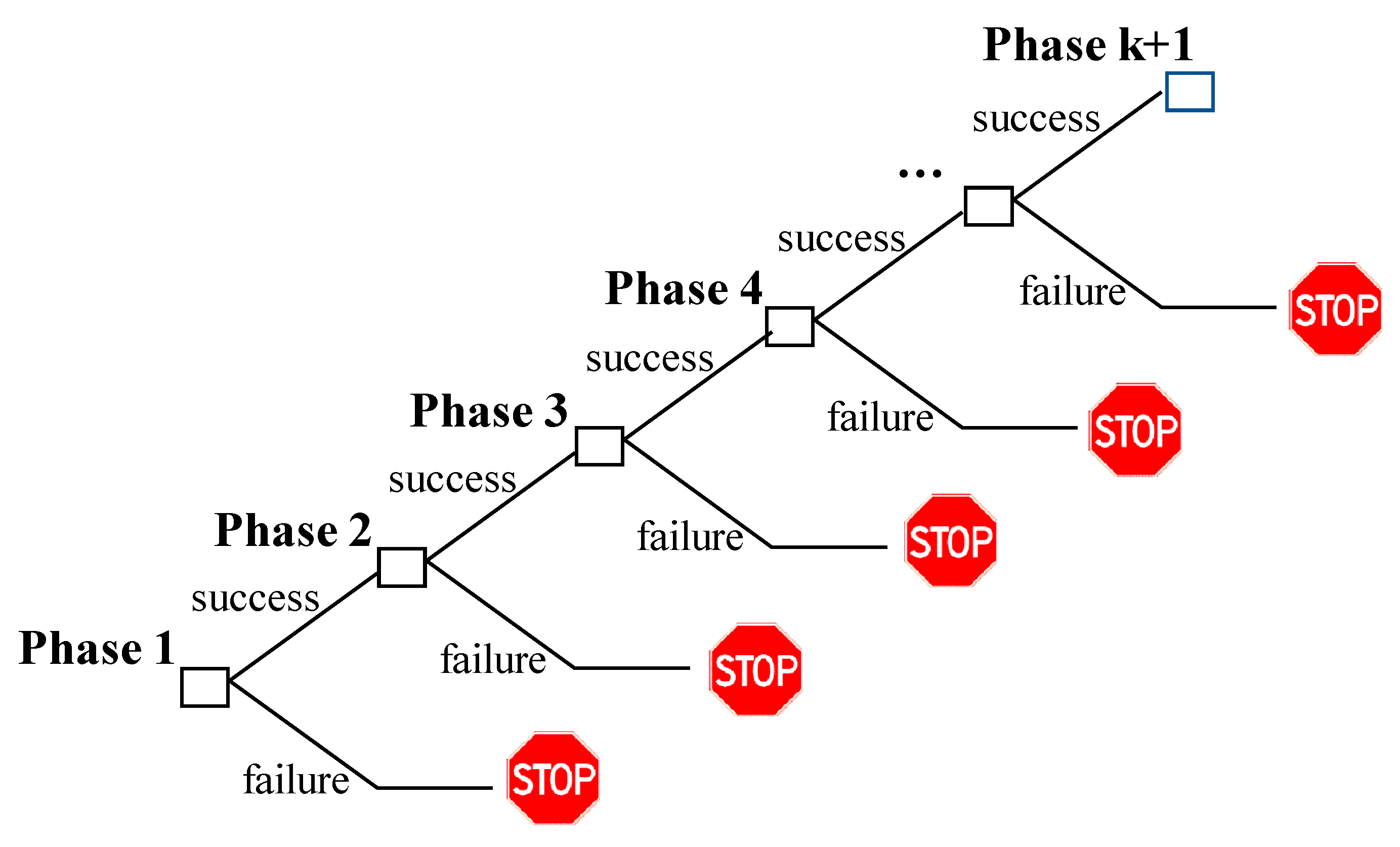
To illustrate the impact of adoption speed on the investment decision, we used the standard N-fold compound real option model of [24,25]. Compound options have been widely used in the financial literature to evaluate sequential investment opportunities. Large-scale capital investments are often sequential and thus require a series of irreversible investments, while significant positive project cash flows are realized only when the whole project is complete. Such an investment process may be interpreted as a sequence of options, such that every investment phase creates an option for an investment in the next phase. If a previous stage turns out to be successful, the next one will be initialized; otherwise, the investment is discontinued. This process goes on until the final stage. Figure 1 visualizes this sequential chains of options.

Following [25], the multistage investment will be priced as a compound option, interpreted as a chain of call options to invest. Let us consider an investor who wants to invest in a project whose commercial phase cannot be launched upon the successful competition of previous $k$ investment stages. Let $T_{k+1}$ be the time of the market launch, when, upon paying the commercialization cost $I_{k+1}$, the firm earns the project value $V$. The project payoff at time $T_{k+1}$ is $\max \left[V-I_{k+1},0\right]$. Let $C_{k+1}\left(V,t\right)$ denote the value at time $t$ of this onefold compound option or single stage investment opportunity. We assume that the commercialization phase is reached upon investing an amount $I_k$, at time period $T_k$, with $T_{k+1}\ge T_k\ge \cdots T_2\ge T_1\ge 0$. The project starts with $I_1$ as the startup costs, while $T_k$ and $I_k$ are maturities of intermediate phases that lead up to the commercialization phase and the respective investment costs. At any stage $k$ the investor can decide to abandon the project or to enter the next stage, hence, the optional nature of the investment project (Figure 2). The multistage investment problem may be viewed as a compound option, that is options on options, and its value may be derived in a recursive way.

A generalized $N$-fold compound option model explicitly incorporating both commercial (market) and technical uncertainty to value sequential multistage investment projects is developed in [25]. Technical uncertainty refers to technical success of each investment stage by multiplying the option value at each decision point with the probability of technical success at that stage. In this model, the project has a commercial risk $\sigma$ and technical success probabilities $p_1,p_2,\dots ,p_{k+1}$ at each investment stage. The project value is unknown and is denoted by $V_t$ at time $t$. It is described by a geometric Brownian motion:

$$d{V}_t=\mu V_{t}dt+\sigma V_{t}d{W}_t,$$

(7)

where $\mu$ and $\sigma$ represent the growth rate and the standard deviation of the project value. The stochastic variable $d{W}_t$ follows a Wiener process with $d{W}_t~N\left(0,\sqrt{dt}\right)$. The term dW_t includes technological risk, market risk (alternative competing technologies), political risk, etc. In this paper, we do not elaborate on these specific risks, nor do we try to model them, as we are primarily interested here in the effect of the interaction between infrastructure availability and demand sensitivity to infrastructure on the project value and on investment decisions. Appendix A explains the N-fold compound option model in more detail.

4. An Application to the Case of Hydrogen Infrastructure in the Netherlands

In this section, we first introduce the setup of the hydrogen infrastructure project in the Netherlands. Subsequently, we develop and discuss the way we adapted the GB model to this particular case. In particular, we show how we modelled the sensitivity of hydrogen cars to available hydrogen infrastructure.

4.1. Description of the Hydrogen Infrastructure Project

The setup of the hydrogen infrastructure project is loosely based on the EU HyWays project [59]. It lays out a phased roadmap for hydrogen stations in 10 European countries, viz. Finland, France, Germany, Greece, Italy, the Netherlands, Norway, Poland, Spain, and the United Kingdom [59]. This hydrogen energy roadmap distinguishes the following four settings with respect to policy support and technical learning: “baseline”, “modest policy support and modest learning”, “high policy support and high learning”, and “very high policy support and high learning”. Here, we took the “modest policy support and modest learning” setting as our starting point.

Furthermore, the roadmap assumes a number of stages. Phase I (2010–2015) was a small scale experimental (pre-commercial) phase which brought up to 10,000 hydrogen vehicles on European roads. Phase II (2015–2020) is the early commercial phase. The roadmap assumes that in the early commercial phase, three to six early user centers will be developed in each country. For the Netherlands, these are the regions around Amsterdam, Rotterdam, and Nijmegen (see [18] for an application on a regional scale). The ambition is to link these national centers through so-called hydrogen corridors. Subsequently, nationwide networks will be rolled out. With respect to the number of required stations, the HyWays roadmap assumes that in the early commercial phase about 400 stations will be necessary in the early user centers, plus another 500 to facilitate the hydrogen corridors. In the full commercialization stage III, an increase is foreseen to 4 million between 2020 and 2025 and to 16 million hydrogen cars after 2025. In the final stage after 2025, 13,000 to 20,000 stations ultimately will be needed to serve ten million hydrogen vehicles.

All of the above numbers are for the total of 10 participating countries, so we needed to scale those numbers to obtain estimates for the Dutch market. When measured in terms of the number of users, the Netherlands accounts for 3.34% of the total target population in the EU, while measured in kilometers of roads they account for 3.95% of the EU total [60]. Taking 4% as the approximate proportion of the Netherlands within the HyWays project, this would correspond to 400 hydrogen cars by 2015, 20,000 cars by 2020, and a further growth to 640,000 after 2025. With respect to the number of stations, the HyWays setup implies that about 30 stations would be built by 2015 and 800 by the end of phase III (compared with the minimum number of hydrogen filling stations for the UK (1198) and California (2085), see [23]). In reality, the objectives of the HyWays scenario have not been realized so far and the project considerably lags behind the 2008 expectations. We nevertheless used its assumptions and original time path for the setup and simulations in this paper.

The timing of achieving those target numbers is dependent on the specific setting underlying the scenario. The number of years for each phase uses the same timing as [18], which comprised of an earlier regional study on one specific Dutch area. The current country-level study on the entire Dutch territory used the same timing for reasons of comparability and was roughly in line with the HyWays scenario. Different phases are obviously possible and our models allows for the calculation of this, but such analysis is outside the confines of the current article. In our analysis, we took a 34 year horizon. We chose the precommercial phase I to run from 2010 until 2014. It comprised of technology refinement and market preparation. The early commercialization phase II is from 2015 until 2024 and the full commercialization phase III from 2025 until 2044. In the real option analysis, we used a proxy for the cash flows after 2044. Subsequently, we designed six different strategies with respect to the timing of investment in infrastructure, leading to different speeds of construction for the refueling stations. In all scenarios, the final number of 800 stations is reached in 2044. At that time hydrogen-fueled vehicles are supposed to be cost effective compared to electric vehicles. Furthermore, we assumed demand (adoption) to be governed by a Bass model.

For some intuition behind these different phases, consider the following. Generally, the introduction of an innovative technology leads to early adoption by enthusiasts. In this case, the pre-commercialization phase would be attained when enough hydrogen stations are in place to satisfy the refueling needs of many early adopters [22,35]. These consumers will be somewhat more willing to be inconvenienced by driving out of their way to refuel with hydrogen. The early commercialization phase is attained when enough hydrogen stations are in place to satisfy a larger portion of the general population. High volume sales to the general public take place in the final, full commercialization phase. Since many consumers want to be able to drive long distances and do not want to be confined to a specific area, a local infrastructure probably will not suffice in this stage anymore. To overcome range anxiety or to avoid congestion at charging or fueling stations, at least a coarse national network would have to be in place [19].

We approached the optimal building strategy in deciding the coarseness of the hydrogen refueling station network from the business-driven perspective of an infrastructure provider. This is a different perspective than most of the literature so far, which has focused on the optimal location of recharging or refueling infrastructure from a planning perspective. For instance, [61] incorporated driving patterns to analyze the optimal location of public charging systems for electric cars in New York City, while [20] performed a similar analysis for hydrogen fueling stations in Seville.

The advantage of a multiphased process is that it allows staged investments and investment decisions. Moreover, it makes a real option analysis an attractive and appropriate approach to assess the attractiveness of the investment. Each stage can be viewed as an option on the value of subsequent stages and valued as a compound option [24,25]. It is important to note that phase III (full commercialization) cannot proceed without the execution and successful completion of phase II, which itself will only take place upon the successful transition from phase I. The end points of phases I and II thus represent decision times (to stop or to continue), in addition to the starting decision at the beginning of stage I for the investor in hydrogen infrastructure. A positive continuation decision at that time requires the option value of the future project to exceed the extra investment required to enter the next phase. If not, the project will be terminated.

To calculate the expected operating cash flows for each project phase, we needed to quantify the present value of the expected operating revenues R_t less operating expenses C_t, which requires a substantial amount of assumptions with respect to the input values of all parameters of the cash flow model. To calculate hydrogen demand for fuel cell passenger vehicles, we assumed that each vehicle will use approximately 0.7 kg of hydrogen each day, amounting to 255.5 kg per year. For an average fuel cell vehicle with a fuel economy of 80 to 96 km per kg, this would accommodate about 56 to 64 km of driving on an average day [62,63]. For hydrogen fuel to be competitive with fossil fuels, the literature generally assumes a retail price of €10/kg [64]. We took into account the regular fuel taxes in the Netherlands, such as excise duty and VAT, which would lower the net retail price to €4/kg.

Although hydrogen is much cheaper produced from natural gas, the production process is always associated with the emission of greenhouse gases and local pollutants [65]. The sustainable hydrogen cost is initially about €5/kg (phase I), but due to technical learning, we assumed it will gradually decrease to €4/kg in phase II and a long-term production cost of €3.4/kg in phase III (adapted from [64,66]). This includes all the relevant expenses, for instance, transportation to the refilling station and carbon capture and storage (CCS) costs if necessary. After 2044, annual operational cash flows are assumed to remain constant forever. Their present value in 2044 was used in the computations as the residual value of the investment.

For the computations, we furthermore used a 25.5 percent marginal tax rate [67], an average Eurozone inflation rate of 2.24% [68], a 1.13% real interest rate, a 21.21% net working capital requirement in a given year (as percentage of the sales) [69], and a straight-line depreciation over the 20 year economic life of each station. We used a risk-adjusted discount rate of 8% for calculating the NPV of the project cash flows. This cost of capital corresponds to the 2010 sector averages of oil and gas distribution (7.19%), environmental (7.62%), natural gas (8.07%), power (8.23%), automotive (8.58%), and chemical (8.88%) [69]. For our real option calculations, we finally needed the input of the volatility of the project return—we used an annual standard deviation of 66.75%, obtained from [18].

Each stage also requires investments in the necessary amount of hydrogen fuel stations in order to operate the fuel network. The cost of a hydrogen fuel station depends upon many factors, including the type of station, location, equipment manufacturing volume, and continuing technology advancements. Here, we based our assumptions on [66]. We assumed a standard hydrogen station initially costs €0.95 million. Unit investment costs will decrease over time as a result of economies of scale and learning. To reflect this, we specified the cost function as $\varpi (N)=\alpha \cdot N^{-b}$, where $\varpi (N)$ is the investment cost of the Nth unit, b is a learning parameter, and α the investment cost of the first unit (€0.95 million). We chose b to be equal to 0.0465, so that the unit costs decrease to €0.70 million by 2044. The average investment cost to build N fuel stations will therefore be equal to $I=a\cdot {\displaystyle \underset{1}{\overset{N}{\int }}{N}^{-b}}dN$. Fixed one-time installation costs amounted to 30 percent of the unit costs and annual maintenance costs were 3.5%. Additional labor costs are €0.5 million per year.

4.2. The Model

In our application, we started from the GB model in Equation (4). However, rather than assuming that x_t is a function of price and marketing effort, we assumed x_t is a function of availability of refueling stations. Put differently, we hypothesized that potential buyers of a hydrogen car—adopters of the new hydrogen technology—will be more inclined to actually buy the car when they know there will be sufficient refueling stations in the region in which they intend to drive the car [19,22]. Specifically, we proposed

$$x_t=1+\beta \frac{N_t-{\overline{N}}_t}{{\overline{N}}_t}$$

(8)

where N_t equals the cumulative number of refueling stations that has been built up until year t and ${\overline{N}}_t$ equals the cumulative number of refueling stations that would have been built up until year t when the same amount of stations would be built every year over the complete 34 year planning horizon. The gap in Equation (8) then indicates how far the actual building—investment—strategy deviates from the constant investment path. Note that when actual investment exactly follows the linear trend, the gap will be zero and x_t will equal one for the whole period. In this “neutral” scenario, the model reduces to the basic Bass model, consistent with the argument of [26].

Further, we defined $\beta$ as the diffusion coefficient that controls the effect of available stations in accelerating and decelerating the diffusion process. The motivation behind this setting was to reflect the importance of refueling infrastructure investments on the market penetration of hydrogen cars. When β equals zero, the sensitivity of adoption to realized stations is zero and the model reduces to the standard Bass model. The higher β, the stronger the effect of early investment on adoption will be. We used the combination of Equations (1), (4), and (8) in our scenario analysis, using different paths for N_t and different parameter values for β. The overall equation thus looks like

$$\frac{dK}{dt}=[p+\frac{q}{\overline{K}}{K}_t][\overline{K}-K_t]*[1+\beta \frac{N_t-{\overline{N}}_t}{{\overline{N}}_t}].$$

(9)

5. A Scenario Analysis

Direct estimation of a simple Bass model or an extended GB model for the hydrogen case is infeasible, due to the lack of actual data on infrastructure investment and consumer adoption. This is similar to many previous disruptive technologies prior to market entry [33]. For that reason, we focused on a scenario analysis.

As discussed previously, we assumed that the rollout of an infrastructure for hydrogen fuel cell vehicles will cover the period 2010–2044. In these 34 years, we assumed 800 fueling stations will be built to service a maximum capacity of 640,000 vehicles ($\overline{K}$). However, the timing of the building process was taken as a free parameter here. The purpose of the scenario exercise was to investigate the impact of different speeds at which the stations are built on the potential profitability of the overall project, taking into account the impact of the building strategy on the adoption speed of hydrogen cars in the market.

We did this by embedding the GB model of Equation (9) into the real option framework. In the following section, we define six plausible investment scenarios, distinguished by the speed at which refueling stations are built. The GB model pins down the diffusion process of adoption through three parameters p, q, and β. For p and q we use constant values across all scenarios, calibrated on the HyWays characteristics [59]. For β we used four different parameter values, reflecting different demand sensitivities with respect to the availability of infrastructure. The higher β, the more weight potential users attach to having easy access the refueling infrastructure in their adoption decision. The results will shed light on the way the optimal investment (building) strategy depends on the sensitivity of adoption to available infrastructure.

5.1. Scenario Assumptions

We took a two-step approach. First, we motivated the six different scenarios. Subsequently, we elaborated on the choice of p, q, and β.

We started from the so-called “neutral” scenario—henceforth labeled Neutral. This is the base scenario in which the stations are built at constant speed over the whole 34 year period. It is constructed as a neutral, steady increase scenario. That is, every year about 24 stations (=800/34) are added to the existing stock of stations. It follows from Equation (9) that in the “neutral” scenario the diffusion process will take the typical S-shaped Bass distribution. In this case the gap variable in x_t is zero throughout the whole period regardless of the value of β, because the investment gap $\raisebox{1ex}{$N_t-{\overline{N}}_t$}\!\left/ \!\raisebox{-1ex}{${\overline{N}}_t$}\right.$ is zero.

Subsequently, we designed a number of other scenarios in which the building speed differs from Neutral. Obviously, an infinite number of scenarios is possible. We chose a grid that has a sufficiently wide range to capture many of the realistic scenarios and appropriately investigate the sensitivity of investment decisions through real option analysis. Note that all scenarios were constrained by the requirement that 800 stations need be built in 34 years. It implies that building scenarios that start slow will have to catch up later on, while scenarios that start fast need to reduce building down the road. Second, we chose for linear building patterns for reasons of tractability and plausibility.

Four scenarios follow a similar pattern, with a linear (constant speed) build-up until 2024 and a second linear path between 2024 and 2044. Cautious has a very slow start with only 50 stations built in the first fourteen years. As a result, building speed has to pick up substantially to build the remaining 750 stations between 2025 and 2044. In Conservative, the number of stations built in the first fourteen years doubles to 100 (compared to Cautious). In Confident, again a doubling takes place, to 200 in the first fourteen years. Note that all of these scenarios still build at a lower speed initially than Neutral. In Neutral, 329 stations are built between 2010 and 2024. Aggressive is the mirror image of Confident relative to Neutral. In Aggressive, 460 stations are built in the first fourteen years, which is as much more relative to Neutral as Confident is less. Finally, Catch-up starts with the same speed as Confident, but accelerates after ten years (in 2020) until it reaches the level of Aggressive in 2034 where it slows down again to follow the latter path. The building strategy in the Conservative scenario roughly equals that of HyWays [59].

Table 1. Building speed per scenario and regime (new stations per year).

Scenario	# of New Stations Built in Each Time Period (The Build-Up is Linear)
	Period 1–34	Period 1–14	Period 14–34	Period 1–10	Period 10–24	Period 24–34	Total
Neutral	800						800
Cautious		50	750				800
Conservative		100	700				800
Confident		200	600				800
Aggressive		460	340				800
Catch-up				143	487	170	800

provides an overview of the build-up per scenario.

Note that the regime changes in the different scenarios do not necessarily coincide with the decision years 2014 and 2024 in the real option analysis. However, we evaluated all scenarios on the basis of these decision points for the infrastructure developer. Figure 3 provides a graphical illustration of the different investment strategies and corresponding growth of the number of refueling stations in the different scenarios.

We now turn to the parameterization of the model. Obviously Bass type models have been used extensively in the literature to model the diffusion of new products and technologies. The Bass model is often used for prediction purposes, where it is well-known that long-run forecasts become more uncertain. In this paper, we were not really aiming at long-run point forecasts of adoption per se. The purpose of the paper was to shed light on the question of how uncertainty, both on the supply side (availability of infrastructure) and on the demand side (sensitivity to availability) and their interaction, impacts on the decision of whether or not to make long-term investment decisions. We used four different specifications of the Bass model as well as six different investment scenarios to capture the range of uncertainty, without claiming—or needing to claim—that one of the forecasted sales time paths is the correct one. Especially for consumer durables, many empirical applications are available, see for example [26,53,70]. Estimates for p typically are in the range from 0 to 0.04, while estimates for q range from around 0.20 to about 0.70. In some applications, the ceiling $\overline{K}$ is pre-specified, in others it is estimated as an extra parameter. Estimation methods include simple OLS, maximum likelihood estimation (MLE), and nonlinear least squares (NLS). We refer to [70] for a comparison and discussion. Moreover, estimation typically requires reformulating Equation (1) or (9) in discrete time. The discrete version of Equation (9) looks as follows

$$d{K}_t=K_t-K_{t-1}=[p+\frac{q}{\overline{K}}{K}_{t-1}][\overline{K}-K_{t-1}]*[1+\beta \frac{N_{t-1}-{\overline{N}}_{t-1}}{{\overline{N}}_{t-1}}].$$

(10)

It allows for the estimation of four parameters, p, q, β, and $\overline{K}$.When β is set to zero, the model reduces to the standard Bass model with three parameters to be estimated.

Due to lack of data, we did not estimate but calibrated the parameters p and q in Equation (10) at 0.004 and 0.275 to allow the diffusion process to converge gradually towards the potential adoption level $\overline{K}$ (640,000) by the year 2044. These values fall into the range usually found when estimating the Bass model. For β we chose four different values reflecting differences in the sensitivity of demand to the availability of refueling stations using the GB model. In particular, we consecutively set the value of β equal to zero, 0.25, 0.50, and 0.75. When β equals zero, the number of available refueling stations plays no role in the consumers’ decision to adopt the new technology and the GB model reduces to the standard Bass model. The higher the value of β, the more important the availability of sufficient refueling stations is for consumers.

5.2. Results

For each combination of a specific scenario and a value of β, we now could compute the adoption speed and corresponding demand for hydrogen vehicles. From this, the time path of costs and revenues and operating cash flows can be computed. These in turn serve as input for the computation of the net present values for each stage, as well as the real option value at the start of the project. The results of this exercise are reported in

Table 2. Comparing scenarios for β = 0.

Scenarios	Net Present Value				Real Option Value
	Phase I	Phase II	Phase III	Total	Option Value	Project Value	Investment Decision	Rank
Neutral	−97	−182	152	−128	136	39	Invest	5
Cautious	−24	−53	76	0	169	145	Invest	1
Conservative	−37	−77	91	−23	161	124	Invest	2
Confident	−64	−124	119	−69	149	85	Invest	3
Aggressive	−130	−241	187	−184	128	−2	Reject	6
Catch-up	−64	−164	141	−87	148	84	Invest	4

,

Table 3. Comparing scenarios for β = 0.25.

Scenarios	Net Present Value				Real Option Value
	Phase I	Phase II	Phase III	Total	Option Value	Project Value	Investment Decision	Rank
Neutral	−97	−182	152	−128	136	39	Invest	5
Cautious	−22	−43	14	−51	123	101	Invest	1
Conservative	−36	−69	41	−64	125	89	Invest	2
Confident	−63	−119	91	−91	129	66	Invest	4
Aggressive	−131	−247	211	−166	145	14	Invest	6
Catch-up	−63	−159	121	−102	133	70	Invest	3

,

Table 4. Comparing scenarios for β = 0.5.

Scenarios	Net Present Value				Real Option Value
	Phase I	Phase II	Phase III	Total	Option Value	Project Value	Investment Decision	Rank
Neutral	−97	−182	152	−128	136	39	Invest	5
Cautious	−21	−36	−62	−119	69	48	Invest	2
Conservative	−35	−62	−18	−116	83	48	Invest	2
Confident	−62	−114	61	−116	108	46	Invest	4
Aggressive	−131	−253	233	−152	159	28	Invest	6
Catch-up	−62	−155	100	−117	121	59	Invest	1

and

Table 5. Comparing scenarios for β = 0.75.

Scenarios	Net Present Value				Real Option Value
	Phase I	Phase II	Phase III	Total	Option Value	Project Value	Investment Decision	Rank
Neutral	−97	−182	152	−128	136	39	Invest	2
Cautious	−20	−31	−150	−201	13	−7	Reject	6
Conservative	−34	−58	−86	−178	38	4	Invest	5
Confident	−62	−110	28	−144	86	24	Invest	4
Aggressive	−132	−260	251	−142	170	38	Invest	3
Catch-up	−62	−152	79	−134	106	44	Invest	1

. Each table corresponds to a different value of β. The results for scenario Neutral were identical across β values as the investment gap equaled zero all the time.

We started with the case of β = 0, where infrastructure availability does not influence adoption speed. Essentially, the GB model reduces to the basic Bass model and adoption only is a function of the parameters p and q. As a result, all scenarios are equal on the revenue side. However, the different scenarios do differ in the speed at which stations are built and, thus, in the time path of cash outflows. The results are provided in Table 2. The first three columns of Table 2 contain the net present values for each investment phase in present value terms: phase I is between year 1 and year 4, phase II is between year 5 and year 14, and phase III is between year 15 and year 34. Column 4 sums these NPVs and gives the overall NPV of the project at its start. According to the NPV criterion, a minimum condition for the project to start is a positive NPV. Column 5 has the real option value of the project today. As the infrastructure project is a multistage investment, we used the n-fold compound option model of [25] to compute the real option values. According to the real option criterion, the project is feasible when the call option value today exceeds the initially required net investment. We assumed this equals the NPV of phase I operating cash flows in present value terms. The project value in column 6 equals the call option value minus the cash flows (required investment) from phase 1. That is, a positive project value implies the option is “in-the-money” and can be exercised to start the project.

A first thing to note from Table 2 (the case of β = 0, where infrastructure availability does not influence adoption speed) is that the NPV analysis would result in rejection of the project, regardless of the specific time path of investments. This is a common result for large infrastructural projects as uncertainty about future revenues is large and upfront investment outlays are high. From a NPV perspective, no infrastructure developer will start the current hydrogen project. This is exactly the reason why real option theory provides an attractive alternative in project assessment. Table 2 shows that the option criterion would only reject the project in the most risky scenario, Aggressive. The scenarios in which investment starts very slowly would do best. This result is not surprising. Since demand (adoption) is insensitive to the availability of infrastructure (β = 0), aggressively and quickly building many stations in the early years does not pay off. It leads to high costs without compensating revenues. Slow investment in the early years reduces costs in the first phase, as can be seen by comparing the Phase I NPV across scenarios in column 1. It puts the scenarios where investment starts more aggressively at a disadvantage.

Table 3, Table 4 and Table 5 have the same design as Table 2 and provide information on the role of higher sensitivity of demand to available refueling stations. In Table 3, β rose to 0.25, suggesting consumer demand is somewhat sensitive to the availability of refueling stations. It remains true that the project would be rejected on the basis of overall NPV, but would be accepted using real option valuation, regardless of the specific building design. In terms of project value, the scenarios converge a bit. Especially the two slow scenarios (Cautious and Conservative) would now have a substantially lower project value, while the project value for Aggressive would increase somewhat. These effects are due to the fact that the faster building scenarios now benefit on the revenue side from faster adoption compared to the slow building scenarios. However the impact is insufficient to alter the ranking of the projects substantially. Only Confident and Catch-up would change places.

When demand sensitivity was increased even more with a β of 0.5, we did see somewhat more of an effect. Table 4 shows that with this value of β, the scenarios would actually converge considerably in overall performance. Differences both in overall NPV and in project value would be relatively small. Catch-up would actually show the best performance. In Table 5, we provide evidence for the case when demand sensitivity is high (β = 0.75). Now, Cautious and Conservative would make up the rear. Actually, the project would be rejected for Cautious and only marginally accepted for Conservative. Since Conservative is the scenario that we derived from the Hyways case, it deserves attention on its own. Interestingly, it would do quite well when there is low demand responsiveness to the availability of infrastructure, but would fall to the bottom of the rankings when demand responsiveness increases.

In this particular setup, the consequences of failing to correctly incorporate the endogeneity of demand in the analysis in terms of inappropriately accepting or rejecting the project at the start are limited. Taking the β = 0 scenario as our benchmark, the results show that with relatively strong demand responsiveness, Aggressive may be incorrectly rejected, while Cautious may be incorrectly accepted—and even deemed optimal. The project would be accepted on the basis of the real option value for all other scenarios for all values of β. However, there is no guarantee decisions would also turn out this way.

Overall, our analysis shows it is important to understand and appropriately model the diffusion process of a new technology like the development of hydrogen vehicles and the corresponding infrastructure. Ignoring the potential interaction between the speed with which the required infrastructure—and for that matter also a sufficient set of attractive vehicles themselves—will become available and the adoption process may lead to suboptimal decisions with respect to the optimal timing of investment spending as well as with respect to the assessment of the feasibility of the project in general.

5.3. Recent Events

When we compare the time line of the fueling network build-up assumed in the original Hyways scenario [59,60], it becomes clear that the initial expectations were never met. Under the original plan, about 30 stations should have been built between 2010 and 2014. Between 2015 and 2024, between 50 and 460 stations should have been built, while the plan assumes 800 stations across the Netherlands at the end of 2044. At the beginning of 2020 only four fueling stations were present in the Netherlands (Groningen, Arnhem, Rotterdam, Helmond). In March 2020, a fifth fueling station was opened in The Hague. It is obvious that in reality the network is far behind the original plan. If we look at the other countries in the original Hyways plan, we observe that countries such as Finland, Greece, and Poland still have no fueling stations, while Spain and Italy only have three stations each. Only the UK (17 stations), France (27 stations), and especially Germany, with a broad network of 89 stations, are doing better (see Figure 4). Overall, the Netherlands ranks at this moment only at the 9th spot of European countries with hydrogen fueling stations. Dutch policymakers in the meantime updated their beliefs on a realistic pathway to developing a hydrogen economy and have launched new policy initiatives [71,72].

In the meantime the European economy has been hit hard due to the outbreak of the COVID-19 outbreak. It is hard to predict how this will impact the development of Dutch and European hydrogen market. On the one hand, increased uncertainty would induce firms to delay investments [73]. This would imply a further delay in the construction of hydrogen fueling stations. If this scenario unfolds, the Dutch fueling network will remain too embryonal for the hydrogen market to take off over the next decade. On the other hand, the call for significant government intervention in the economy after the COVID crisis is very predominant. This is especially the case to support sustainable energy solutions [74]. The EU’s Green Deal to reduce carbon emission might results in a faster scaling up of hydrogen fueling networks across Europe than was the case before the pandemic [75].

The most successful development of a hydrogen infrastructure network can be found outside of Europe. At the end of May 2020, Japan had a network of 111 stations (see Figure 5). The first station was opened in 2003, while the second was only put in use in 2010. As of 2014 the development of a hydrogen fueling network started taking off aggressively due to a strategic plan of the Japanese government [76]. This has caused a very rapid increase in the number of stations: 27 in 2015, 49 in 2016, and 12 in 2017 (see Figure 5). This was probably only possible with the dedicated support of the Japanese industry, for instance, from car producers such as Toyota and Nissan who commercialized hydrogen cars, but also from the energy subsidiaries of large industry players, such as Toshiba or Kawasaki, in developing hydrogen as an energy carrier [77]. Although plans exist for the construction of 24 new stations (situation in June 2020), it remains unclear when they will be actually constructed. It becomes clear that the momentum seems lost as the construction of new hydrogen fueling stations slowed down significantly after 2018. Even though Japan had plans to build an additional 50 stations in 2020, with the aim to have a wider network ready for the August 2020 Olympic Games in Tokyo [78], it remains unclear whether the current slowdown is due to COVID-19 or is more of a structural problem.

6. Conclusions

In this paper, we explicitly incorporated the impact that realized investments in new infrastructure may have on the adoption speed in a real options framework for taking investment decisions under uncertainty and analyzing the consequences of this interdependence for optimal business investment strategies. The investment in fueling stations for hydrogen vehicles has the characteristics of a chicken–egg problem: without sufficient infrastructure, consumers will not adopt the new technology; but without (likely) adoption, investors will not build the infrastructure. To address the issue of choosing an optimal investment path when adoption depends on previous investments in the necessary infrastructure, we combined a real option modeling approach with a modified generalized Bass model for the adoption diffusion process.

As an illustration, we applied the combined model to the case study of the introduction of infrastructure investments for fueling stations for hydrogen vehicles in the Netherlands. We performed a scenario analysis where we combined six different investment strategies with four different parameterizations of the GB model. We assumed that the number of available refueling stations—relative to a linear trend—is a key driver of the diffusion model that captures the adoption decision. The variation in parameterization captured different degrees of demand sensitivity to existing infrastructure.

Our results show that it is important to understand and appropriately model the diffusion process of a new technology, like the development of hydrogen vehicles and the corresponding infrastructure. Ignoring the potential interaction between the speed with which the required infrastructure—and for that matter also a sufficient set of attractive vehicles themselves—will become available and the adoption process may lead to suboptimal decisions with respect to the optimal timing of investment spending as well as with respect to the assessment of the feasibility of the project in general.

If policymakers want to stimulate the emergence of sustainable energy solutions, such as hydrogen, they need to be aware of the importance of the interaction between demand and supply. When designing policies or roadmaps for a hydrogen economy, explicitly incorporating the impact of the size and coverage of the network of fueling stations on the adoption speed of consumers is a key dimension to successfully induce private investors to make optimal investments. Without such explicit attention, there is a significant challenge in matching the scale and timing of the fueling infrastructure investment with the actual hydrogen demand. Policymakers are recommended to invest in studies to estimate the sensitivity of consumer demand to available infrastructure. Based on demand studies, policymakers can develop pathways for optimal market penetration and use it to support the timely takeoff of hydrogen infrastructure. For instance, our results show that with relatively strong demand responsiveness, one pathway would have been incorrectly rejected, while another pathway would have been incorrectly accepted. By estimating demand responsiveness more accurately, a more effective pathway could be chosen to support the takeoff of hydrogen infrastructure investments.

Although our study shows interesting exploratory results, more research is needed to obtain realistic estimates of the magnitude of the relevant parameters that govern the adoption diffusion process for new technologies in order to guide policymakers and private investors better. We call upon researchers to focus more attention to this aspect of our modeling approach.