Abstract
In recent years, gross domestic product (GDP) has grown rapidly in China, but the growth rate of carbon dioxide (CO2) emissions has begun to decline. Some scholars have put forward the environmental Kuznets curve (EKC) hypothesis for CO2 emissions in China. This paper utilized the panel data of 30 provinces in China from 1997 to 2016 to verify the EKC hypothesis. To explore the real reasons behind the EKC, the index gasoline to diesel consumption ratio (GDCR) was introduced in this paper. The regression results showed that CO2 emissions and GDP form an inverted U-shaped curve. This means that the EKC hypothesis holds. The regression results also showed that a 1% GDCR increase was coupled with a 0.118186% or 0.114056% CO2 emission decrease with the panel fully modified ordinary least squares or panel dynamic ordinary least squares method, respectively. This means that CO2 emissions negatively correlate with GDCR. From the discussion of this paper, the growth rate reduction of CO2 emissions is caused by the economic transition in China. As changes of GDCR can, from a special perspective, reflect the economic transition, and as GDCR is negatively correlated with CO2 emissions, GDCR can sometimes be used as a new socioeconomic indicator of carbon dioxide emissions in China.
1. Introduction
There is considerable evidence proving that global warming is very likely to be caused by carbon dioxide (CO2) emissions and fossil fuel consumption is the main reason for CO2 emissions [1,2]. In the past 30 years, China has experienced rapid growth in its economy and energy consumption. The problem of CO2 emissions has become much more important for China [3].
In recent years, the gross domestic product (GDP) still grows rapidly in China, but the growth rate of CO2 emissions has begun to decline for the whole of China and for some Chinese provinces [3]. Based on this, some scholars have hypothesized that the CO2 emissions in China will form an inverted U-shaped curve with respect to GDP [4,5,6]. This hypothesis is called the environmental Kuznets curve (EKC) for CO2 emissions in China.
This paper utilized the panel data from 1997 to 2016 of 30 provinces in China to verify the EKC hypothesis. To investigate the real reasons behind EKC and the underlying motivation of the reduction of the CO2 emission growth rate, a new index—the gasoline to diesel consumption ratio (GDCR)—was introduced in this paper. The index, GDCR, means the ratio of gasoline consumption to diesel consumption of a particular region. In China, as passenger cars almost always use gasoline and commercial vehicles almost always use diesel, the changes of GDCR can reflect the economic transition in China. If the industrial economy grows, the usage of commercial vehicles (especially heavy trucks) will increase, so diesel consumption will increase and GDCR will decrease; if the service economy grows, the usage of passenger cars will increase, gasoline consumption will increase, and GDCR will increase. Therefore, from the perspective of the transportation utilization of different economic sectors, the changes of GDCR can reflect the economic transition in China, and the reflection of GDCR to economic structure is quite different from using the output value to represent the economic structure. The output value is only one of the dimensions, and the output value alone cannot represent the reason of the structural change of CO2 emissions. GDCR also cannot represent the change of CO2 emissions, but it can provide a new perspective for CO2 emission studies. Moreover, if the correlation between GDCR and CO2 emissions can be verified, GDCR may become a new indicator of CO2 emissions.
Figure 1 shows the historical data of the GDP, CO2 emissions, GDCR, diesel consumption, and gasoline consumption of the whole of China from 1997 to 2016. As shown in Figure 1, the CO2 emission growth rate began to decrease from 2011 with the rapid growth of GDP; GDCR formed a U-shaped curve over time, which was just the opposite of the CO2 emissions.
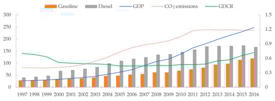
Figure 1.
GDP, CO2 emissions, gasoline to diesel consumption rate (GDCR), diesel consumption, and gasoline consumption of China in 1997–2016. (Data source: National Bureau of Statistics in China. Note: to show in one figure, the unit of gasoline and diesel are million tons, the unit of GDP is 3 × 10¹¹ RMB (Unit of Chinese money), the unit of CO2 emissions is 5 × 10⁷ tons, and the unit of GDCR is 1).
The initial idea of this paper was generated from plant optimization research for refineries. In the oil refining industry, the gasoline to diesel production ratio (GDPR) is an important index for facilities and for refineries. Refineries have to work hard to adjust the GDPR to meet the GDCR. In this research, we found that GDCR is influenced by changes in economic structure and can reflect the economic transition. Once we started to study the EKC for CO2 emissions in China, we thought of the index GDCR and began to consider the relationship between CO2 emissions and GDCR. This is the initial idea of this paper.
Previous studies of EKC for CO2 emissions have revealed the inverse U-shaped curve of CO2 emissions and GDP in China, but they have failed to reveal precisely all the indicators of CO2 emissions and they do not use GDCR. This paper has introduced GDCR, and this is the main innovation of this paper. This paper will combine the environmental Kuznets curve of GDCR and CO2 emissions to prove the correlation between GDCR and CO2 emissions. This paper assumes that GDCR will be negatively correlated with CO2 emissions. In other words, the increase of gasoline consumption will reduce China’s CO2 emissions, and the reduction of diesel consumption will reduce China’s CO2 emissions. Therefore, GDCR becomes a new socioeconomic indicator of carbon dioxide emissions in China.
2. Literature Review
The concept of the Kuznets curve was introduced by Kuznets [7] to describe the inverted U-shaped relationship of income inequality and economic growth. From the 1990s, the Kuznets curve was used in pollutant emission studies. Grossman and Krueger [8] first proposed that pollutant emissions and per capita income form an inverted U-shaped curve. Panayotou [9] first used the term EKC to name this phenomenon. Since then, the EKC has been investigated by many scholars [10]. Among them, Dinda [11] pointed out that the economic transition and fortune changes of a country and people’s increasing preference for environmental quality are the real reasons for the EKC.
Following its initial use for environmental quality, EKC was used to research CO2 emissions; this kind of research was called EKC for CO2 emissions. Moomaw and Unruh [12] first used EKC to study CO2 emissions and GDP. Using data from 16 countries, they demonstrated that CO2 emissions also prove a third-order polynomial relation, an N-shaped curve with GDP, in addition to a second-order polynomial relation, a U-shaped curve. This means that whether the curve is U-shaped or N-shaped may not be decided by the data, but by the type of the econometric model that has been selected. Subsequently, Sun [13] said that the EKC for CO2 emissions merely reflected the peak theory of energy intensity. Sun’s view could explain some fundamental influence of energy efficiency on CO2 emissions, but obviously his paper did not consider the impact of economic transitions and energy transitions on CO2 emissions. After these early studies, many different empirical studies of EKC for CO2 emissions were conducted for various countries and regions. Using the panel data of five regions in Canada from 1970 to 2000, Lantz [14] studied the non-linear relationship between CO2 emissions and their influencing factors, and proved that CO2 emissions had nothing to do with per capita GDP, but had an inverted U-shaped relationship with population and a U-shaped relationship with technology. Saboori [15] used the data of Malaysia from 1980 to 2009 to verify the hypothesis of the environmental Kuznets curve, and proved that the relationship between carbon dioxide emissions and GDP is inverted U-shaped, which supports the EKC hypothesis. Galeotti [16] proved that the carbon emissions of OECD (Organization for Economic Co-operation and Development) countries are in line with EKC, while non-OECD countries show different situations according to different data sources. Using panel data from 11 OECD countries, Iwata [17] studied the role of nuclear energy in the environmental Kuznets curve of CO2 emissions, and proved that Finland, Japan, South Korea, and Spain meet the EKC hypothesis, and also that nuclear energy can only reduce CO2 emissions for some countries. Using data from 19 European countries, Acaravci [18] demonstrated the environmental Kuznets curve for carbon dioxide emissions in Denmark, Germany, Greece, Iceland, Italy, Portugal, and Switzerland. Using the data of 12 countries in the Middle East and North Africa (MENA) from 1981 to 2005, Arouri [19] proved that the hypothesis of environmental Kuznets curve holds for CO2 emissions of MENA, but the turning point is very low and the inverted U-shaped relationship is not obvious. To summarize the above, generally speaking, the hypothesis of the environmental Kuznets curve of CO2 emissions may be true for high-income countries, but not for low-income countries.
In recent years, as China has become a major carbon dioxide emitter, the EKC for CO2 emissions in China has attracted much scholarly research. Kang, Zhao, and Yang [5] used panel data from the years 1997–2012 from Chinese provinces and compared the non-spatial and the spatial panel models. They found that Eastern China has had a sharper increase in CO2 emissions than Western China and that, compared to urbanization and coal consumption, trade has had little effect on CO2 emissions. Using provincial-level data of 1995–2014 in China, Dong, Sun, Hochman, Zeng, Li, and Jiang [4] not only examined the EKC for CO2 emissions, but also investigated the influence of natural gas consumption on CO2 emissions. They found that the EKC appears mainly for Eastern and Central provinces in China, and natural gas consumption shows a positive influence on CO2 emission reduction.
All the above papers are about EKC, but to research the impact factors and indicators of CO2 emissions, some scholars have tried from other perspectives and used other kinds of models. Among them, Fan, et al. [20] used the stochastic impacts by regression on population, affluence, and technology (STIRPAT) model and found that population, income, and energy intensity (technology) correlated strongly with CO2 emissions. Li et al. [21] used the STIRPAT model and found that GDP, population, urbanization, economic structure, and technology level were factors impacting CO2 emissions. Wang et al. [22] used an extended STIRPAT model and found that population, GDP, technology level, urbanization, economic structure, energy structure, and foreign trade were factors impacting CO2 emissions. To summarize the studies of the impact factors of CO2 emissions, there were some similarities of these studies. They used the same kind of models, either the STIRPAT model or the extended STIRPAT model; they found similar impact factors of CO2 emissions, population, income (or GDP), energy intensity (technology level), urbanization, industrial structure, energy structure, foreign trade, and so on.
Another kind of reference of this paper are the studies of the gasoline to diesel consumption ratio (GDCR). When it comes to the literature review of the gasoline to diesel ratio, as far as we know, most of the papers with the keywords of either the gasoline to diesel ratio or diesel to gasoline ratio (or something like this) can be divided into two categories. One category is about the research of blended combustion for the internal combustion engine [23,24]. The other category is about the research of product optimization for oil processing [25,26]. The research with the keywords of the ratio of gasoline to diesel ratio (or something like this) seldom belongs to the field of macroeconomics. Chang and Zhang [27] found that emission allowance prices exhibit co-movement with diesel and gasoline prices in China using the GARCH (generalized autoregressive conditional heteroskedasticity) method with Copula function. Dahl [28] studied the price elasticity and income elasticity of gasoline and diesel, and gave policy suggestions for more than 100 countries. Karagiannis et al. [29] tested the short-term and long-term conduction effect of crude oil prices to gasoline and diesel retail prices in Germany, France, Italy, and Spain, but above all, their studies did not use the ratio of gasoline to diesel, or even the ratio of the price of gasoline and diesel. We have not yet found any macroeconomic research about GDCR.
In summary, previous research on EKC and CO2 emissions have made a lot of achievements and have used various kinds of data and regression methods. However, the actual problem of finding the real reason behind EKC has not been solved. To the best of our knowledge, the relevant literature has not introduced the index of GDCR into the EKC and CO2 emissions studies. Based on this, this paper introduces the GDCR.
3. Methodology
3.1. Variables
To verify the EKC hypothesis, this paper chose CO2 emissions per capita as the dependent variable and GDP per capita and its square as independent variables [30]. Because CO2 emissions are influenced by the economic transition and GDCR can reflect the economic transition from the perspective of transportation needs, GDCR was also chosen as one of the independent variables.
3.2. Model
Quantitative regression was used in the empirical study of this paper, and the first-order linear equation was chosen as the regression model. According to the selection of variables mentioned above, the econometric model is shown in Formula (1).
PCCDE represents per capita CO2 emissions; PCGDP represents the per capita GDP; ln denotes the logarithm of the data; (ln PCGDP)2 represents the square of the logarithm of PCGDP; GDCR represents the gasoline to diesel consumption ratio; a, b, and c are the parameters that need to be estimated; and r is the residue of estimation.
In the regression results, if the parameter of the GDP square was negative, that means that CO2 emissions and GDP formed an inverted U–shaped curve, so the EKC hypothesis held [31]; if the parameter of GDCR was negative, that means GDCR was negatively correlated with CO2 emissions.
3.3. Data
There are 34 provinces in China, but the data of Hong Kong, Macao, Taiwan, and Tibet were vacant, so this paper used panel data of 30 provinces from 1997 to 2016 in China. The data source was the National Bureau of Statistics, China. The data of CO2 emissions were calculated mainly using the method proposed by Dong, Sun, Hochman, Zeng, Li, and Jiang [4], with some modification: Dong’s method calculated CO2 emissions by end-side energy consumption data, whereas this paper used the primary energy consumption data. The data of GDP used the unit of RMB (Unit of Chinese money), and they were normalized to 1997 prices. The statistic table, distribution curve, and scatter plot of the data are shown in Table 1 and Figure 2. As shown in Table 1, the number of observations was 600 and the statistical description of variables, such as standard deviation, kurtosis, and skewness, can be viewed from Table 1 and Figure 2.

Table 1.
Statistic table of variables from 30 China provinces from 1997–2016.
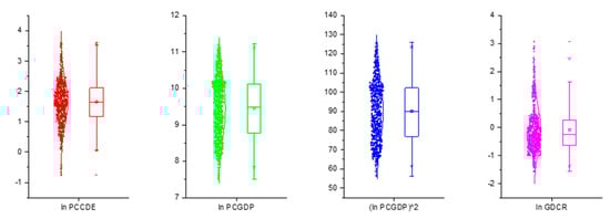
Figure 2.
Box chart of variables from 30 China provinces in 1997–2016.
3.4. Statistical Test and Parameter Estimation
In order to test the stability of the sample sequence, the variables were subjected individually to the LLC (Levin-Lin-Chu) unit root test and the ADF-Fisher test in level and first difference, respectively. If the variables passed the LLC and ADF-Fisher tests, the variables were stationary. Then, all the variables together were subjected to a panel Padron co-integration test [32]. If the variables passed the panel Padron co-integration test, that means that there were co-integration vectors between variables and the variables could be regressed. The estimation methods used in this paper were the method of panel fully modified ordinary least squares (FMOLS) [33] and panel dynamic ordinary least squares (DOLS) [34].
4. Results and Discussion
4.1. Results of Unit Root Test
Table 2 shows the results of the unit root test by the LLC method and the ADF–Fisher method. Only “ln PCGDP” and “(ln PCGDP)2” passed the LLC test at levels, and all variables passed the LLC test and ADF-fisher test at first difference. This means that all variables were stationary at first difference.
Table 2.
Results of unit root test.
4.2. Results of Co-Integration Test
The results of the unit root test showed that all variables were stationary at first difference. Then, they were subjected to a Pedroni co-integration test; the results are shown in Table 3. For the model with the intercept, five of the seven results negated the non-co-integration hypothesis with a 95% confidence level. Hence, there was a long-term co-integration relationship among CO2 emissions, GDP, and GDCR.
Table 3.
Results of panel Pedroni co-integration test.
4.3. Results of Parameter Estimation
As the test results show, the panel data of the China provinces passed the co-integration test. Table 4 shows the results of the parameter estimation obtained by the FMOLS method and the DOLS method. The regression results of the panel data showed that the CO2 emissions formed an inverted U-shaped curve with respect to GDP. This means that the EKC hypothesis held.
Table 4.
Parameters of long-run estimation of China provinces and panel data.
The regression results of the panel data also showed that a 1% GDCR increased couples with 0.118186% or 0.114056% decreases in CO2 emissions by the panel fully modified ordinary least squares (FMOLS) or panel dynamic OLS (DOLS) method, respectively. This means that GDCR negatively correlated with CO2 emissions.
For 30 provinces in China, the regression results were quite different. Figure 3 shows the colored map of various provinces; Figure 3a,b show the relationship between GDP and CO2 emissions; Figure 3c,d show the relationship between GDCR and CO2 emissions. Figure 3 shows a colored map of China’s provinces. In Figure 3a,b, in the green provinces, the CO2 emissions formed an inverted U-shaped curve with respect to GDP. In the red provinces, the CO2 emissions formed a U-shaped curve, and in the yellow provinces, the CO2 emissions formed neither an inverted U-shaped curve nor a U-shaped curve, but an approximately linear line. In Figure 3c,d, in the green provinces, the CO2 emissions had a negative correlation with GDCR. In the red provinces, the CO2 emissions had a positive correlation with GDCR, and in the yellow provinces, the correlation between CO2 emissions and GDCR was neither negative nor positive, but irrelevant.
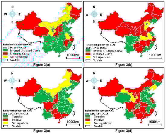
Figure 3.
Colored maps of China provinces that reflect the estimation results. Note: the “not significant” means that the absolute value of the parameter of GDP square or GDCR was less than 0.1, and that means the impact of the variable on CO2 emissions was not significant, which were signed as “not significant”).
4.4. Results of Residual Test
The residuals of the FMOLS and DOLS were subjected to a unit root test, LLC, ADF-Fisher, and PP-Fisher. The results of the residual stationarity test are shown in Table 5. As shown in Table 5, the residuals of the FMOLS and DOLS passed the unit root test. Therefore, the residuals were stationary sequences, proving the real existence of the co-integration relationship between variables.
Table 5.
Results of residual stationarity test.
4.5. Discussion
From the regression results, some meaningful conclusions can be drawn. Firstly, as GDCR can represent the economic transition and GDCR correlates strongly with CO2 emissions, to some extent, GDCR becomes a new socioeconomic indicator of CO2 emissions in China. Other discussions are shown as follows.
(1) Relationship of CO2 emissions and GDP is independent from the value of GDP
When studying the EKC for CO2 emissions in China, Dong [4] points out that the existence of EKC has nothing to do with the per capita GDP of each province. As a result of this paper, Table 6 shows the types of result curves of CO2 emissions and GDP, the turning point of EKC, and the GDP of the years 1997 and 2016. Figure 4 shows the scatter plots of Table 6. The horizontal axis of Figure 4 shows whether the CO2 emissions of a province conform to the Kuznets curve, and the vertical axis of Figure 4 shows the per capita GDP of the province. In Figure 4, no matter whether the amount of the GDP of an individual province is large or small, the result curve will be either a U-shaped curve or an inverse U-shaped curve, and no matter whether the result curve is U-shaped or inverse U-shaped, the amount of GDP may be either large or small. This means that the relationships between CO2 emissions and GDP are independent from the amount of GDP.
Table 6.
The types of regression curves, turning point, and GDP.
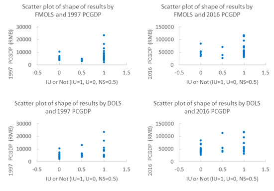
Figure 4.
Scatter plot of the type of result curves and PCGDP. Note: IU means inverted U-shaped. U means U-shaped, NS means not significant. PCGDP means GDP per capita (YUAN, nominal GDP per capita).
(2) Relationship of CO2 emissions and GDP are associated with economic transition
When studying EKC for air pollutant emissions, Dinda [11] pointed out that a country’s fortunes change—for example, from a clean agrarian economy to a polluting industrial economy to a clean service economy—is the real reason for the EKC. Table 7 shows the relationship between CO2 emissions and GDP, the relationship between CO2 emissions and GDCR, and the percentage of the GDP of various industries of 1997 and 2016.
Table 7.
Regression results and economic structure.
Considering the change of the percentage of each industry of an individual province shown in Table 7, the 30 provinces in China can be classified into five categories. This classification is shown in Table 8. In Table 8, each category corresponds to a unique form of economic transition. The classification of provinces is actually the classification of the mode of economic transition.
Table 8.
Classification of 30 provinces in China by type of economic transition.
The relationship between CO2 emissions and GDP in the regression results can be partly explained by this classification. In the economic transition from agriculture to industry (A2I), the CO2 emissions will increase with GDP growth; in the economic transition from industry to service (I2S), the CO2 emissions will be decrease with GDP growth. For an individual province, if it experiences the I2S after the A2I, the regression curve of this province will be inverted U–shaped, and that means the EKC hypothesis holds for this province. For provinces with other modes of economic transition, the U-shaped curve or inverted U-shaped curve can be explained for similar reasons, and the details are shown in Table 9. Table 9 shows the relationship of regression curves and economic transition modes. In Table 9, each particular mode of economic transition corresponds to some particular modes of regression curves. That means the type of the regression curve of CO2 emissions and GDP are associated with the economic transition.
Table 9.
Relationship of regression curve and economic transition mode.
(3) Negative correlations of CO2 emissions and GDCR are because of economic transition
If a province is in the economic transition from agriculture to industry, diesel consumption will grow faster than gasoline consumption, so GDCR decreases but CO2 emissions will increase because of the industrialization. Thus, CO2 emissions have a negative correlation with GDCR.
For the same reason, if a province is in the economic transition from industry to service, gasoline consumption will grow faster than diesel consumption, so GDCR increases but CO2 emissions decrease because of the economic transition. Thus, CO2 emissions also have a negative correlation with GDCR. These rules are shown in Table 10. As shown in Table 10, for provinces that are experiencing economic transition from agriculture to industry, such as Fujian and Qinghai, the GDCR of these provinces will decrease, and the CO2 emissions will increase, so the correlation of GDCR and CO2 emissions is negative. This is similar for provinces that are experiencing economic transition from industry to service.
Table 10.
Relationship between economic transition and correlation of GDCR and CO2 emissions.
5. Conclusions
Data of recent years show that the growth rate of CO2 emissions has declined for the whole of China and some of the China provinces. This paper utilized the panel data to verify the EKC hypothesis. To explore the real reason behind EKC and the underlying motivation of the growth rate reduction of CO2 emissions, the index GDCR was introduced in this paper. The index, GDCR, means the ratio of gasoline consumption to diesel consumption of a particular region. This paper combines the environmental Kuznets curve for CO2 emissions and GDCR to prove the correlation between GDCR and CO2 emissions. The conclusions are as follows.
- (1)
- The EKC hypothesis for CO2 emissions holds in China.
- (2)
- GDCR can be a new socioeconomic indicator of CO2 emissions in China.
- (3)
- The relationship between CO2 emissions and GDP is independent from GDP.
- (4)
- The relationship of CO2 emissions and GDP is associated with economic transition.
- (5)
- The negative correlation of CO2 emissions and GDCR is because of economic transition.
In summary, this paper shows that the EKC hypothesis holds. This means that CO2 emissions may decrease with GDP growth, but GDP growth is a necessary—but not sufficient—condition for CO2 emission reduction. CO2 emissions are not determined by GDP, but associated with economic transition. Thus, to effectively decrease CO2 emissions and to solve the problem of global warming, the government still needs to formulate relevant policies to transform the economic structure of China.
This paper also has some deficiencies. This paper has only focused on the impact of economic transition, but fails to reflect the impact of energy transition and energy efficiency. In future research, we will study the impact of energy transition and energy efficiency on CO2 emissions further.
Author Contributions
Z.L. provided the initial ideas of this paper, processed the data, conducted the statistical tests and made the econometric regressions. Z.L. also wrote the initial draft. R.S. is the supervision of this reasearch. He designed the methodology and he obtained the financial support for the project leading to this publication. M.Q. and D.H. helped collect the data, made some figures and tables and participated in the editing of this paper. All authors have read and agreed to the published version of the manuscript.
Funding
This research was funded by Chinese National Funding of Social Sciences (No. 17BGL014).
Acknowledgments
We are very grateful to Kang-yin Dong for his help. The authors also gratefully acknowledge the help from the editors and reviewers.
Conflicts of Interest
The authors declare no conflict of interest.
References
- Olivier, J.G.J.; Peters, J.A.H.W.; Janssens-Maenhout, G.; Muntean, M. Trends in Global CO2 Emissions; PBL Netherlands Environmental Assessment Agency: Hague, The Netherlands, 2013. [Google Scholar]
- Nejat, P.; Jomehzadeh, F.; Taheri, M.M.; Gohari, M.; Abd. Majid, M.Z. A global review of energy consumption, CO2 emissions and policy in the residential sector (with an overview of the top ten CO2 emitting countries). Renew. Sustain. Energy Rev. 2015, 43, 843–862. [Google Scholar] [CrossRef]
- Wang, Q.; Wu, S.-D.; Zeng, Y.-E.; Wu, B.-W. Exploring the relationship between urbanization, energy consumption, and CO2 emissions in different provinces of China. Renew. Sustain. Energy Rev. 2016, 54, 1563–1579. [Google Scholar] [CrossRef]
- Dong, K.; Sun, R.; Hochman, G.; Zeng, X.; Li, H.; Jiang, H. Impact of natural gas consumption on CO2 emissions: Panel data evidence from China’s provinces. J. Clean. Prod. 2017, 162, 400–410. [Google Scholar] [CrossRef]
- Kang, Y.-Q.; Zhao, T.; Yang, Y.-Y. Environmental Kuznets curve for CO2 emissions in China: A spatial panel data approach. Ecol. Indic. 2016, 63, 231–239. [Google Scholar] [CrossRef]
- Riti, J.S.; Song, D.; Shu, Y.; Kamah, M. Decoupling CO2 emission and economic growth in China: Is there consistency in estimation results in analyzing environmental Kuznets curve? J. Clean. Prod. 2017, 166, 1448–1461. [Google Scholar] [CrossRef]
- Kuznets, S. Economic Growth and Income Inequality. Am. Econ. Rev. 1955, 45, 1–28. [Google Scholar]
- Grossman, G.M.; Krueger, A.B. Environmental Impacts of a North American Free Trade Agreement; National Bureau of Economic Research: Cambridge, MA, USA, 1991. [Google Scholar]
- Panayotou, T. Empirical Tests and Policy Analysis of Environmental Degradation at Different Stages of Economic Development; International Labour Organization: Geneva, Switzerland, 1993. [Google Scholar]
- Yandle, B.; Vijayaraghavan, M.; Bhattarai, M. The Environmental Kuznets Curve: A Primer; Property and Environment Research Center: Bozeman, MT, USA, 2002. [Google Scholar]
- Dinda, S. Environmental Kuznets Curve Hypothesis: A Survey. Ecol. Econ. 2004, 49, 431–455. [Google Scholar] [CrossRef]
- Moomaw, W.R.; Unruh, G.C. Are environmental Kuznets curves misleading us? The case of CO2 emissions. Environ. Dev. Econ. 1997, 2, 451–463. [Google Scholar] [CrossRef]
- Sun, J.W. The nature of CO2 emission Kuznets curve. Energy Policy 1999, 27, 691–694. [Google Scholar] [CrossRef]
- Lantz, V.; Feng, Q. Assessing income, population, and technology impacts on CO2 emissions in Canada: Where’s the EKC? Ecol. Econ. 2006, 57, 229–238. [Google Scholar] [CrossRef]
- Saboori, B.; Sulaiman, J.; Mohd, S. Economic growth and CO2 emissions in Malaysia: A cointegration analysis of the Environmental Kuznets Curve. Energy Policy 2012, 51, 184–191. [Google Scholar] [CrossRef]
- Galeotti, M.; Lanza, A.; Pauli, F. Reassessing the environmental Kuznets curve for CO2 emissions: A robustness exercise. Ecol. Econ. 2006, 57, 152–163. [Google Scholar] [CrossRef]
- Iwata, H.; Okada, K.; Samreth, S. Empirical study on the determinants of CO2 emissions: Evidence from OECD countries. Appl. Econ. 2012, 44, 3513–3519. [Google Scholar] [CrossRef]
- Acaravci, A.; Ozturk, I. On the relationship between energy consumption, CO2 emissions and economic growth in Europe. Energy 2010, 35, 5412–5420. [Google Scholar] [CrossRef]
- Arouri, M.E.H.; Ben Youssef, A.; M’Henni, H.; Rault, C. Energy consumption, economic growth and CO2 emissions in Middle East and North African countries. Energy Policy 2012, 45, 342–349. [Google Scholar] [CrossRef]
- Fan, Y.; Liu, L.-C.; Wu, G.; Wei, Y.-M. Analyzing impact factors of CO2 emissions using the STIRPAT model. Environ. Impact Assess. Rev. 2006, 26, 377–395. [Google Scholar] [CrossRef]
- Li, H.; Mu, H.; Zhang, M.; Gui, S. Analysis of regional difference on impact factors of China’s energy—Related CO2 emissions. Energy 2012, 39, 319–326. [Google Scholar] [CrossRef]
- Wang, P.; Wu, W.; Zhu, B.; Wei, Y. Examining the impact factors of energy-related CO2 emissions using the STIRPAT model in Guangdong Province, China. Appl. Energy 2013, 106, 65–71. [Google Scholar] [CrossRef]
- Yu, H.; Liang, X.; Shu, G.; Sun, X.; Zhang, H. Experimental investigation on wall film ratio of diesel, butanol/diesel, DME/diesel and gasoline/diesel blended fuels during the spray wall impingement process. Fuel Process. Technol. 2017, 156, 9–18. [Google Scholar] [CrossRef]
- Pinazzi, P.M.; Hwang, J.; Kim, D.; Foucher, F.; Bae, C. Influence of injector spray angle and gasoline-diesel blending ratio on the low load operation in a gasoline compression ignition (GCI) engine. Fuel 2018, 222, 496–505. [Google Scholar] [CrossRef]
- Kassargy, C.; Awad, S.; Burnens, G.; Kahine, K.; Tazerout, M. Experimental study of catalytic pyrolysis of polyethylene and polypropylene over USY zeolite and separation to gasoline and diesel-like fuels. J. Anal. Appl. Pyrolysis 2017, 127, 31–37. [Google Scholar] [CrossRef]
- Suiuay, C.; Sudajan, S.; Katekaew, S.; Senawong, K.; Laloon, K. Production of gasoline-like-fuel and diesel-like-fuel from hard-resin of Yang (Dipterocarpus alatus) using a fast pyrolysis process. Energy 2019, 187, 115–967. [Google Scholar] [CrossRef]
- Chang, K.; Zhang, C. Asymmetric dependence structure between emissions allowances and wholesale diesel/gasoline prices in emerging China’s emissions trading scheme pilots. Energy 2018, 164, 124–136. [Google Scholar] [CrossRef]
- Dahl, C.A. Measuring global gasoline and diesel price and income elasticities. Energy Policy 2012, 41, 2–13. [Google Scholar] [CrossRef]
- Karagiannis, S.; Panagopoulos, Y.; Vlamis, P. Are unleaded gasoline and diesel price adjustments symmetric? A comparison of the four largest EU retail fuel markets. Econ. Model. 2015, 48, 281–291. [Google Scholar] [CrossRef]
- Chen, L.; Chen, S. The Estimation of Environmental Kuznets Curve in China: Nonparametric Panel Approach. Comput. Econ. 2015, 46, 405–420. [Google Scholar] [CrossRef]
- Rashid Gill, A.; Viswanathan, K.K.; Hassan, S. The Environmental Kuznets Curve (EKC) and the environmental problem of the day. Renew. Sustain. Energy Rev. 2018, 81, 1636–1642. [Google Scholar] [CrossRef]
- Pedroni, P. Critical Values for Cointegration Tests in Heterogeneous Panels with Multiple Regressors. Oxf. Bull. Econ. Stat. 1999, 61, 653–670. [Google Scholar] [CrossRef]
- Pedroni, P. Fully Modified OLS for Heterogeneous Cointegrated Panels; Department of Economics, Williams College: Williamstown, MA, USA, 2000. [Google Scholar]
- Lin, B.; Benjamin, I.N. Causal relationships between energy consumption, foreign direct investment and economic growth for MINT: Evidence from panel dynamic ordinary least square models. J. Clean. Prod. 2018, 197, 708–720. [Google Scholar] [CrossRef]


© 2020 by the authors. Licensee MDPI, Basel, Switzerland. This article is an open access article distributed under the terms and conditions of the Creative Commons Attribution (CC BY) license (http://creativecommons.org/licenses/by/4.0/).