Figure 1.
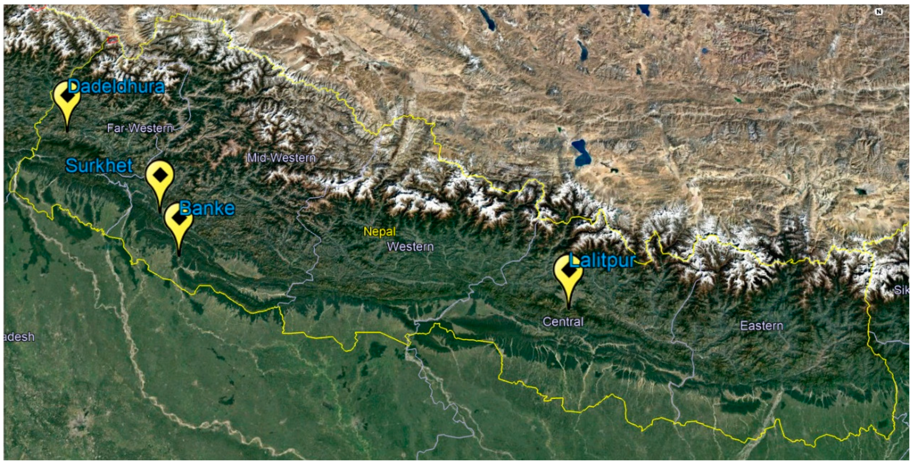
Map showing investigated areas of on-farm experiments in Nepal.
Figure 1.
Map showing investigated areas of on-farm experiments in Nepal.
Figure 2.
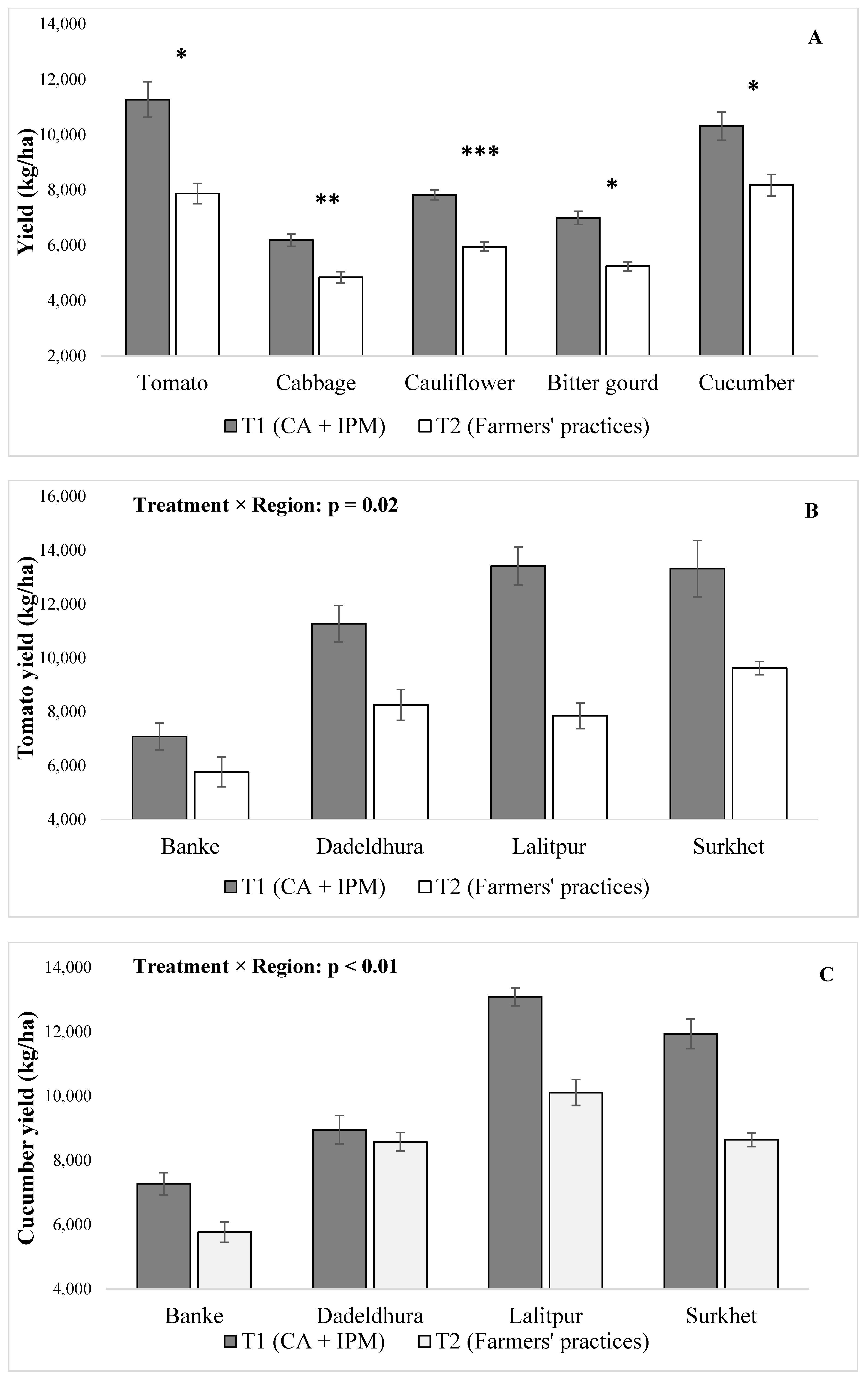
Differences in vegetable crop yields in T1 (improved alternative system; solid bars) vs. T2 (conventional system; open bars) (A) Average yield (kg/ha) for five vegetable crops: tomato, cabbage, cauliflower, bitter gourd, and cucumber in T1 vs. T2. Bars are mean ± standard errors, and means with *, **, ***, are statistically different at probability values of p ≤ 0.05, ≤ 0.01, and ≤ 0.001, respectively. Differences are between “T1” and “T2” within each crop species. (B) Yield differences in tomatoes segregated by four regions: Banke, Dadeldhura, Lalitpur, and Surkhet. Bars are mean ± SEM with significant treatment and region interactions. (C) Yield differences in cucumbers segregated by four regions: Banke, Dadeldhura, Lalitpur, and Surkhet. Bars are mean ± SEM with significant treatment and region interactions.
Figure 2.
Differences in vegetable crop yields in T1 (improved alternative system; solid bars) vs. T2 (conventional system; open bars) (A) Average yield (kg/ha) for five vegetable crops: tomato, cabbage, cauliflower, bitter gourd, and cucumber in T1 vs. T2. Bars are mean ± standard errors, and means with *, **, ***, are statistically different at probability values of p ≤ 0.05, ≤ 0.01, and ≤ 0.001, respectively. Differences are between “T1” and “T2” within each crop species. (B) Yield differences in tomatoes segregated by four regions: Banke, Dadeldhura, Lalitpur, and Surkhet. Bars are mean ± SEM with significant treatment and region interactions. (C) Yield differences in cucumbers segregated by four regions: Banke, Dadeldhura, Lalitpur, and Surkhet. Bars are mean ± SEM with significant treatment and region interactions.
Figure 3.
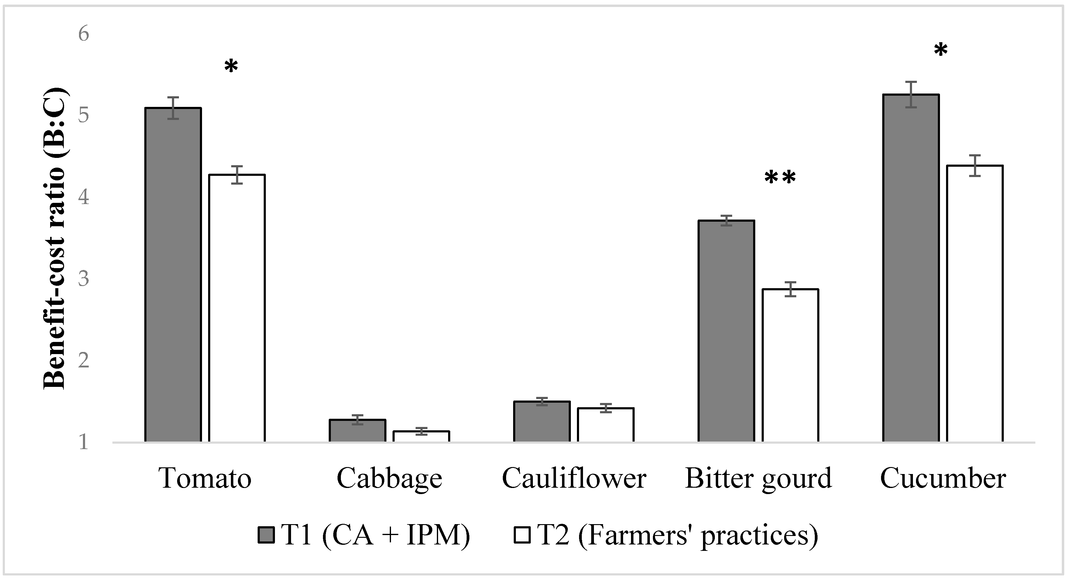
Average benefit–cost ratios (B:C ratio) for five vegetable crops: tomato, cabbage, cauliflower, bitter gourd, and cucumber in T1 (improved alternative system; solid bars) vs. T2 (conventional system; open bars). Bars are mean ± standard errors, and means with *, **, are statistically different at probability values of p ≤ 0.05, ≤ 0.01, and ≤ 0.001, respectively. Differences are between “T1” and “T2” within each crop species.
Figure 3.
Average benefit–cost ratios (B:C ratio) for five vegetable crops: tomato, cabbage, cauliflower, bitter gourd, and cucumber in T1 (improved alternative system; solid bars) vs. T2 (conventional system; open bars). Bars are mean ± standard errors, and means with *, **, are statistically different at probability values of p ≤ 0.05, ≤ 0.01, and ≤ 0.001, respectively. Differences are between “T1” and “T2” within each crop species.
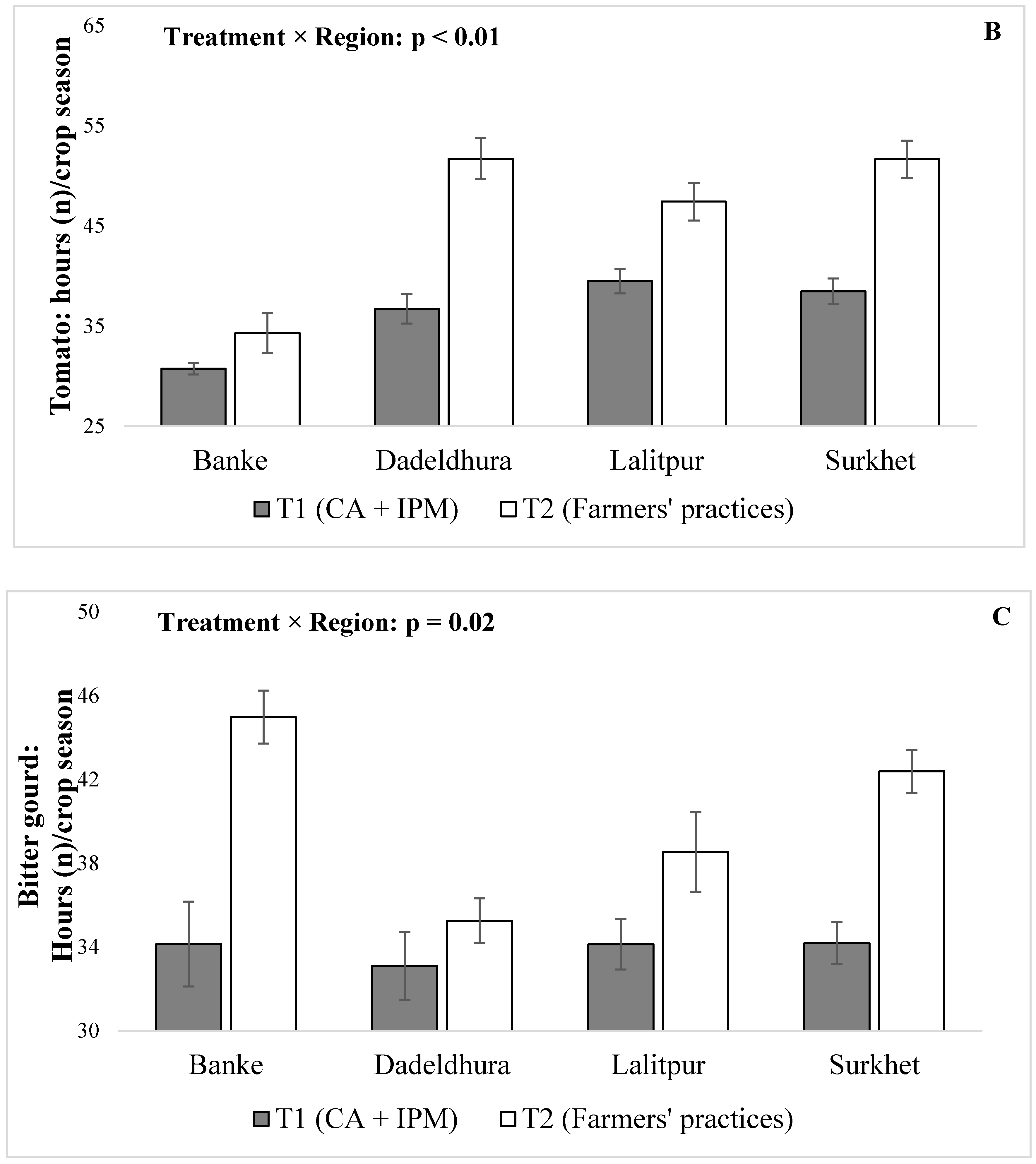
Figure 4.
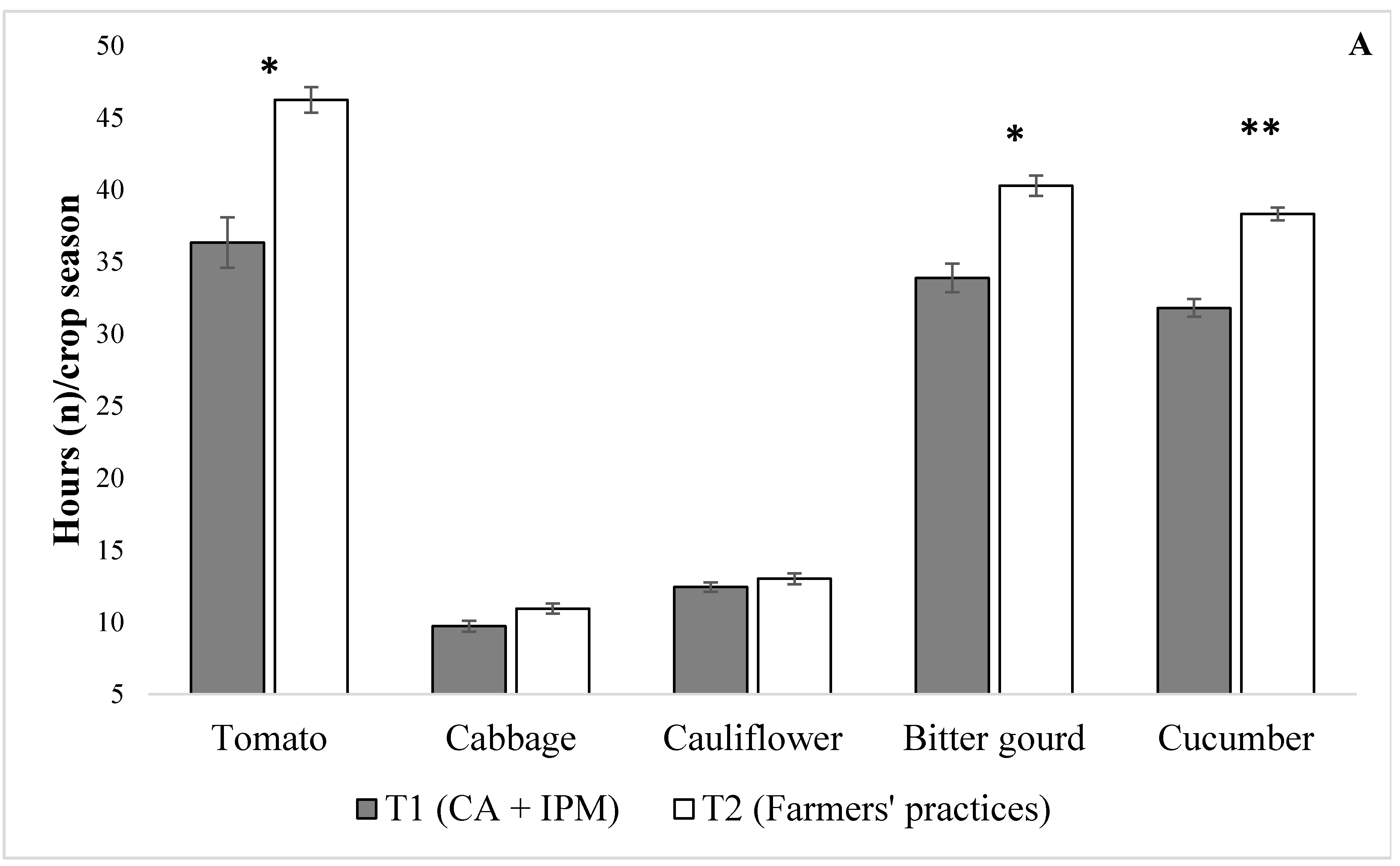
Differences in labor requirement for vegetable crops in T1 (improved alternative system; solid bars) vs. T2 (conventional system; open bars) (A) Average hours of labor/season to manage five vegetable crops: tomato, cabbage, cauliflower, bitter gourd, and cucumber in T1 (improved alternative system; solid bars) vs. T2 (conventional system; open bars). Bars are mean ± standard errors, and means with *, ** are statistically different at probability values of p ≤ 0.05 and ≤ 0.01 respectively. Differences are between “T1” and “T2” within each crop species. (B) Average hours of labor/season in tomatoes segregated by four regions: Banke, Dadeldhura, Lalitpur, and Surkhet. Bars are mean ± SEM with significant treatment and region interactions. (C) Average hours of labor/season in bitter gourds segregated by four regions: Banke, Dadeldhura, Lalitpur, and Surkhet. Bars are mean ± SEM with significant treatment and region interactions.
Figure 4.
Differences in labor requirement for vegetable crops in T1 (improved alternative system; solid bars) vs. T2 (conventional system; open bars) (A) Average hours of labor/season to manage five vegetable crops: tomato, cabbage, cauliflower, bitter gourd, and cucumber in T1 (improved alternative system; solid bars) vs. T2 (conventional system; open bars). Bars are mean ± standard errors, and means with *, ** are statistically different at probability values of p ≤ 0.05 and ≤ 0.01 respectively. Differences are between “T1” and “T2” within each crop species. (B) Average hours of labor/season in tomatoes segregated by four regions: Banke, Dadeldhura, Lalitpur, and Surkhet. Bars are mean ± SEM with significant treatment and region interactions. (C) Average hours of labor/season in bitter gourds segregated by four regions: Banke, Dadeldhura, Lalitpur, and Surkhet. Bars are mean ± SEM with significant treatment and region interactions.
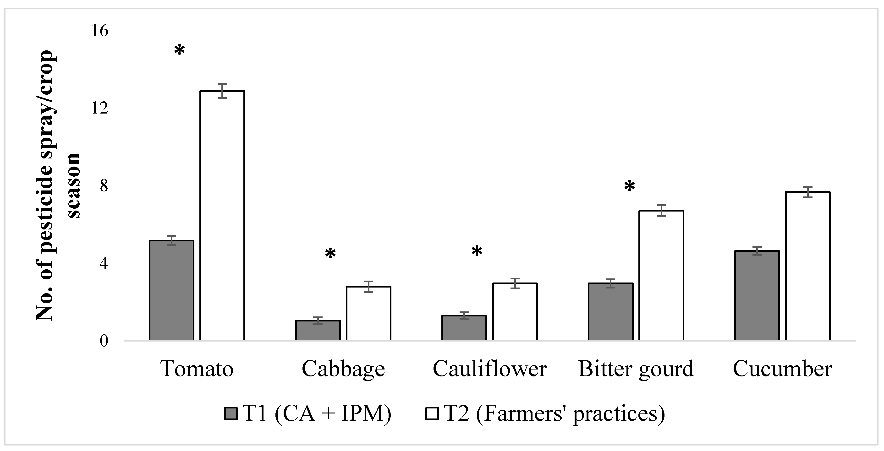
Figure 5.
Average chemical pesticide spray/season on five vegetable crops: tomato, cabbage, cauliflower, bitter gourd, and cucumber in T1 (improved alternative system; solid bars) vs. T2 (conventional system; open bars). Bars are mean ± standard errors and means with * are statistically different at probability values of p ≤ 0.05, respectively. Differences are between “T1” and “T2” within each crop species.
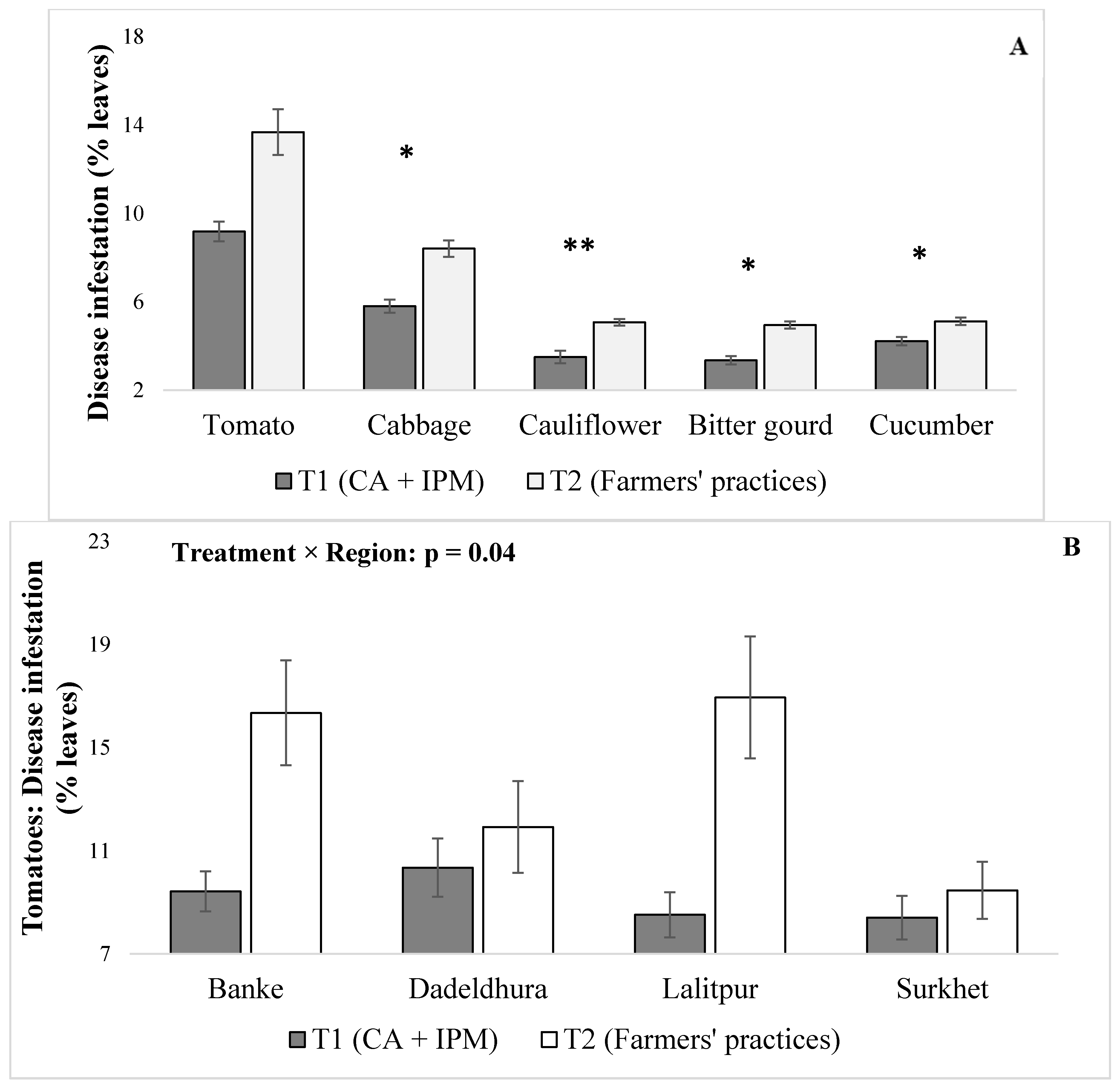
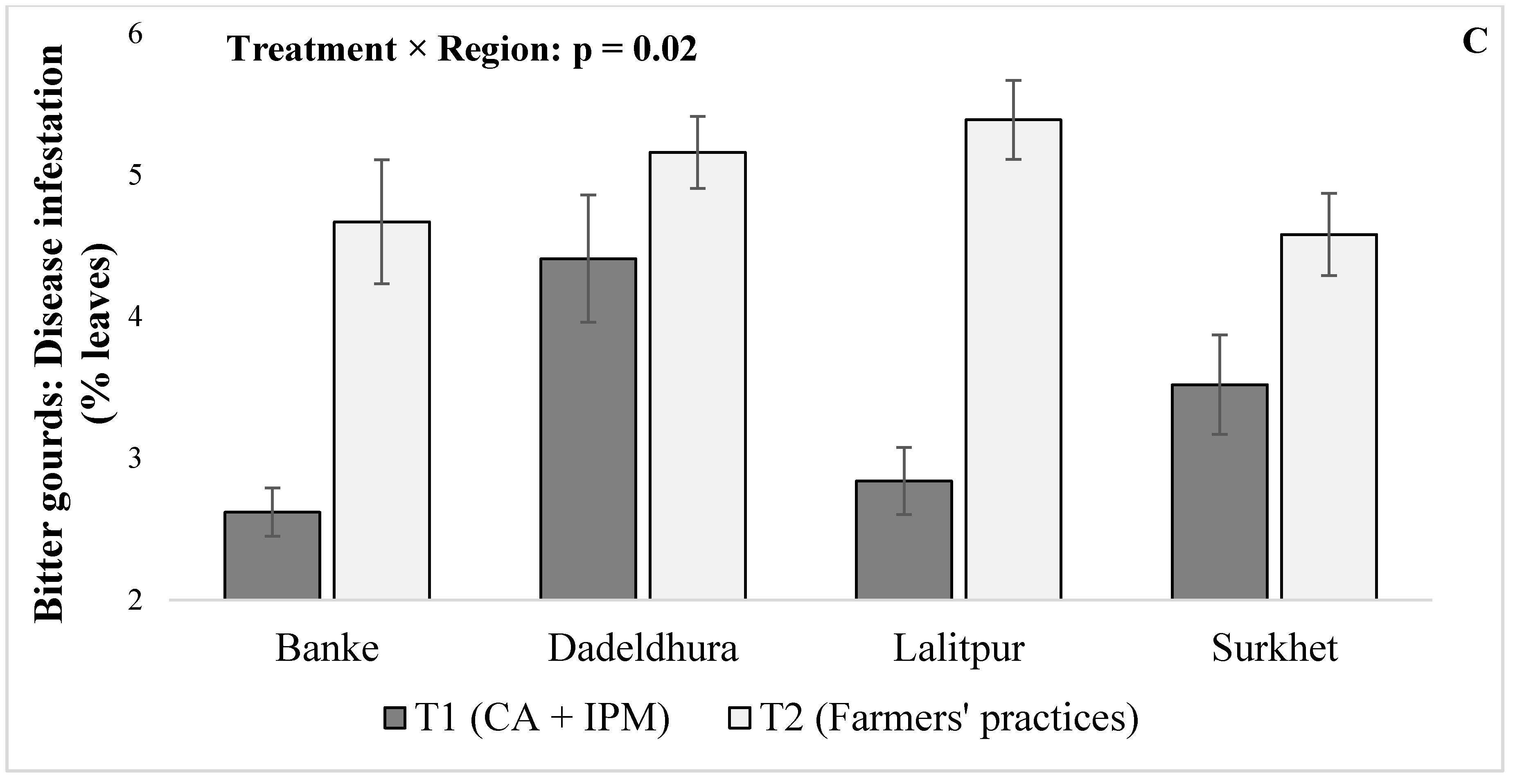
Figure 6.
Differences in disease infestation in vegetable crops in T1 (improved alternative system; solid bars) vs. T2 (conventional system; open bars) (A) Percentage of disease infestation on leaves of five vegetable crops: tomato, cabbage, cauliflower, bitter gourd, and cucumber in T1 (improved alternative system; solid bars) vs. T2 (conventional system; open bars). Bars are mean ± standard errors, and means with *, ** are statistically different at probability values of p ≤ 0.05 and ≤ 0.01, respectively. Differences are between “T1” and “T2” within each crop species. (B) Percentage of disease infestation on tomato leaves segregated by four regions: Banke, Dadeldhura, Lalitpur, and Surkhet. Bars are mean ± SEM with significant treatment and region interactions. (C) Percentage of disease infestation on bitter gourd leaves segregated by four regions: Banke, Dadeldhura, Lalitpur, and Surkhet. Bars are mean ± SEM with significant treatment and region interactions.
Figure 7.
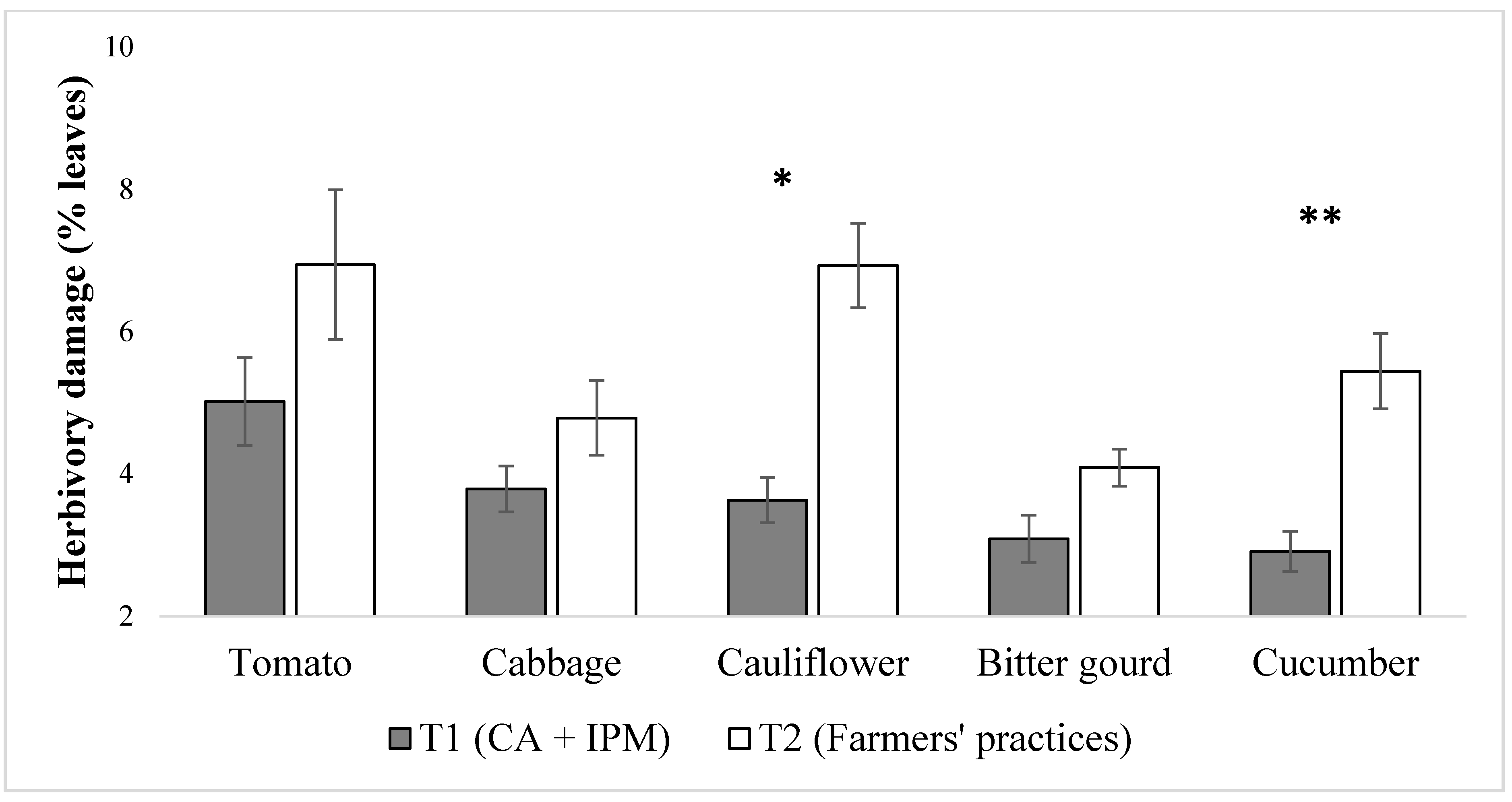
Percentage of herbivory damage on leaves of five vegetable crops: tomato, cabbage, cauliflower, bitter gourd, and cucumber in T1 (improved alternative system; solid bars) vs. T2 (conventional system; open bars). Bars are mean ± standard errors, and means with *, **, ***, are statistically different at probability values of p ≤ 0.05 and ≤ 0.01 respectively. Data were arcsine square root transformed before analysis. Differences are between “T1” and “T2” within each crop species.
Figure 7.
Percentage of herbivory damage on leaves of five vegetable crops: tomato, cabbage, cauliflower, bitter gourd, and cucumber in T1 (improved alternative system; solid bars) vs. T2 (conventional system; open bars). Bars are mean ± standard errors, and means with *, **, ***, are statistically different at probability values of p ≤ 0.05 and ≤ 0.01 respectively. Data were arcsine square root transformed before analysis. Differences are between “T1” and “T2” within each crop species.
Table 1.
Physical characteristics of the investigated sites including elevation, average temperature and rainfall, soil characteristics, and cropping pattern for previous years.
Table 1.
Physical characteristics of the investigated sites including elevation, average temperature and rainfall, soil characteristics, and cropping pattern for previous years.
| Location | Elevation (m) | Avg. Annual Temp. (°C) | Avg. Annual Rainfall (mm) | Soil Characteristics | Cropping Pattern (Previous Years) |
|---|
| Texture | pH |
|---|
| Lalitpur | 1796 | 18.10 | 1505 | Sandy loam | Slightly alkaline (7.35 to 7.45) | Tomato-Cole crops-Chilly/Cole crops/leafy vegetables |
| Banke | 169 | 27.00 | 1312 | Clayey loam | Neutral to slightly alkaline (7.00 to 7.40) | Tomato-Cole crops-Cucurbits |
| Surkhet | 943 | 24.50 | 765 | Sandy loam | Neutral to slightly alkaline (7.00 to 7.40) | Tomato-Cole crops/Wheat-Cucurbits/Leafy vegetables |
| Dadeldhura | 1533 | 16.10 | 1399 | Silty clay | Slightyl alkaline (7.35 to 7.45) | Tomato-Maize-Fallow |
Table 2.
Common crop management practices used for both the improved alternative system (T1) and conventional farmers’ practice (T2). Organic manure was prepared locally using farm wastes and crop residues.
Table 2.
Common crop management practices used for both the improved alternative system (T1) and conventional farmers’ practice (T2). Organic manure was prepared locally using farm wastes and crop residues.
| Crop | Planting Dates | Spacing (Rows × Plants) | Nutrient Application (Chemical Fertilizers) | Organic Manure |
|---|
| Tomato | April–May | 75 × 60 cm | Urea, Diammonium phosphate (DAP) and Murate of potash (MOP) at the rate of (@) 200:140:140 kg/ha; 50% of Urea and 100% of DAP and MOP before planting during land preparation; two split doses of remaining Urea after 20 days of transplanting and at the time of fruiting | 30,000 kg/ha |
| Cabbage | August–September | 50 × 45 cm | Urea, DAP and MOP @ 100:140:100 kg/ha; 50% of Urea and 100% of DAP and MOP before planting during land preparation; two split doses of remaining Urea after 25 and 50 days of transplanting | 25,000 kg/ha |
| Cauliflower | August–September | 60 × 45 cm | Urea, DAP and MOP @ 100:140:100 kg/ha; 50% of Urea and 100% of DAP and MOP before planting during land preparation; two split doses of remaining Urea after 25 and 50 days of transplanting | 25,000 kg/ha |
| Cucumber | March–April | 1 × 1.2 m | Urea, DAP and MOP @ 100:100:100 kg/ha; 50% of Urea and 100% of DAP and MOP before planting during land preparation; two split doses of remaining Urea after 20 and 50 days of transplanting | 20,000 kg/ha |
| Bitter gourd | March–April | 1.5 × 1 m | Urea, DAP and MOP @ 60:100:80 kg/ha; 50% of Urea and 100% of DAP and MOP before planting during land preparation; two split doses of remaining Urea after 20 and 50 days of transplanting | 20,000 kg/ha |
Table 3.
Analysis of variance (ANOVA) table for “yield”; values with asterisk *, **, ***, are statistically different at probability values of p ≤ 0.05, ≤ 0.01 and ≤ 0.001, respectively.
Table 3.
Analysis of variance (ANOVA) table for “yield”; values with asterisk *, **, ***, are statistically different at probability values of p ≤ 0.05, ≤ 0.01 and ≤ 0.001, respectively.
| Crop | Treatment | Region | Treatment × Region |
|---|
| Tomato | 0.03 * | 0.08 | 0.02 * |
| Cabbage | 0.01 ** | 0.05 | 0.52 |
| Cauliflower | 0.001 *** | 0.14 | 0.78 |
| Bitter gourd | 0.01 * | 0.09 | 0.11 |
| Cucumber | 0.05 * | 0.04* | 0.001 *** |
Table 4.
Analysis of variance (ANOVA) table for “benefit—cost ratio (B:C)”; values with *, **, are statistically different at probability values of p ≤ 0.05, ≤ 0.01, and ≤ 0.001, respectively.
Table 4.
Analysis of variance (ANOVA) table for “benefit—cost ratio (B:C)”; values with *, **, are statistically different at probability values of p ≤ 0.05, ≤ 0.01, and ≤ 0.001, respectively.
| Crop | Treatment | Region | Treatment × Region |
|---|
| Tomato | 0.00 ** | 0.05 | 0.54 |
| Cabbage | 0.15 | 0.17 | 0.26 |
| Cauliflower | 0.37 | 0.72 | 0.28 |
| Bitter gourd | 0.00 ** | 0.37 | 0.46 |
| Cucumber | 0.04 * | 0.50 | 0.20 |
Table 5.
Analysis of variance (ANOVA) for “labor”; values with asterisk *, ** are statistically different at probability values of p ≤ 0.05, ≤ 0.01, and ≤ 0.001, respectively.
Table 5.
Analysis of variance (ANOVA) for “labor”; values with asterisk *, ** are statistically different at probability values of p ≤ 0.05, ≤ 0.01, and ≤ 0.001, respectively.
| Crop | Treatment | Region | Treatment × Region |
|---|
| Tomato | 0.03 * | 0.11 | 0.00 ** |
| Cabbage | 0.17 | 0.22 | 0.08 |
| Cauliflower | 0.21 | 0.26 | 0.69 |
| Bitter gourd | 0.04 * | 0.38 | 0.02 * |
| Cucumber | 0.00 ** | 0.46 | 0.42 |
Table 6.
Analysis of variance (ANOVA) table for “spray frequency”; values with *, are statistically different at probability values of p ≤ 0.05, ≤ 0.01, and ≤ 0.001, respectively.
Table 6.
Analysis of variance (ANOVA) table for “spray frequency”; values with *, are statistically different at probability values of p ≤ 0.05, ≤ 0.01, and ≤ 0.001, respectively.
| Crop | Treatment | Region | Treatment × Region |
|---|
| Tomato | 0.00 * | 0.75 | 0.78 |
| Cabbage | 0.00 * | 0.71 | 0.53 |
| Cauliflower | 0.02 * | 0.28 | 0.45 |
| Bitter gourd | 0.00 * | 0.79 | 0.78 |
| Cucumber | 0.07 | 0.96 | 0.87 |
Table 7.
Analysis of variance (ANOVA) table summary with p-values for disease infestation; Values with *, ** are statistically different at probability values of p ≤ 0.05, ≤ 0.01, and ≤ 0.001, respectively.
Table 7.
Analysis of variance (ANOVA) table summary with p-values for disease infestation; Values with *, ** are statistically different at probability values of p ≤ 0.05, ≤ 0.01, and ≤ 0.001, respectively.
| Crop | Treatment | Region | Treatment × Region |
|---|
| Tomato | 0.10 | 0.50 | 0.04 * |
| Cabbage | 0.03 * | 0.82 | 0.13 |
| Cauliflower | 0.00 ** | 0.84 | 0.87 |
| Bitter gourd | 0.03 * | 0.41 | 0.02 * |
| Cucumber | 0.01* | 0.12 | 0.70 |
Table 8.
Analysis of variance (ANOVA) table summary with p-values for herbivory damage; Values with *, ** are statistically different at probability values of p ≤ 0.05, ≤ 0.01, and ≤ 0.001, respectively.
Table 8.
Analysis of variance (ANOVA) table summary with p-values for herbivory damage; Values with *, ** are statistically different at probability values of p ≤ 0.05, ≤ 0.01, and ≤ 0.001, respectively.
| Crop | Treatment | Region | Treatment × Region |
|---|
| Tomato | 0.14 | 0.12 | 0.88 |
| Cabbage | 0.30 | 0.76 | 0.25 |
| Cauliflower | 0.05 * | 0.80 | 0.10 |
| Bitter gourd | 0.08 | 0.28 | 0.39 |
| Cucumber | 0.02 ** | 0.40 | 0.39 |

 ,
, 


