Abstract
The integrated character of the sustainable development goals in Agenda 2030, as well as research in environmental security, flag that sustainable peace requires sustainable and conflict-sensitive natural resource use. The precise relationship between the risk for violent conflict and natural resources remains contested because of the interplay with socio-economic variables. This paper aims to improve the understanding of natural resources’ role in the risk of violent conflicts by accounting for complex interactions with socio-economic conditions. Conflict data was analysed with machine learning techniques, which can account for complex patterns, such as variable interactions. More commonly used logistic regression models are compared with neural network models and random forest models. The results indicate that a country’s natural resource features are important predictors of its risk for violent conflict and that they interact with socio-economic conditions. Based on these empirical results and the existing literature, we interpret that natural resources can be root causes of violent intrastate conflict, and that signals from natural resources leading to conflict risk are reflected in and influenced by interacting socio-economic conditions. More specifically, the results show that variables such as access to water and food security are important predictors of conflict, while resource rents and oil and ore exports are relatively less important than other natural resource variables, contrasting what prior research has suggested. Given the potential of natural resource features to act as an early warning for violent conflict, we argue that natural resources should be included in conflict risk models for conflict prevention.
1. Introduction
Both peace and sustainable natural resource management are integral parts of the interlinked Sustainable Development Goals of Agenda 2030 [1]. Concerns about the effect of unsustainable natural resource use on violent conflict have been expressed by the field of environmental security since the 1990s. Homer-Dixon [2] demonstrated in the early 1990s with six case studies how natural resource scarcities lead to violent conflict and thereby opened the scientific discussion. He concluded that violence due to natural resource scarcity ‘will usually be sub-national, persistent, and diffuse’ [2] (p. 6). Sachs and Warner [3] statistically showed that natural resource abundance hinders development and termed this process the ‘resource curse’. Later, Lujala [4] showed that resource-rich countries experienced higher risks for violent conflict. Collier and Hoeffler [5] and Le Billon [6] investigated the mechanisms behind the resource curse, using econometrics and case-study approaches respectively. On the one hand, finances from natural resource exploitation support rebellion. On the other hand, a largely resource dependent economy presents serious governmental challenges to avoid grievances over unequal distribution of revenues.
Current trends impacting natural resources, such as increased consumption [7], climate change [8], and environmental degradation [9], heighten the urgency to understand the exact mechanisms how natural resource use drives risk for violent conflicts. Barnett and Adger [10] claim that environmental change causes security problems by reducing access to and the quality of natural resources to sustain livelihoods. On a more international scale, Klare [11] explains how upcoming resource shortages will increase competition between countries and corporations. In general, the field of environmental security informs that sustainable resource management is necessary for sustainable peace and vice versa.
Furthermore, practitioners and policy makers have acknowledged the link between natural resources and risk for violent conflict. In 2008, an EU-UN partnership on Land, Natural Resources and Conflict Prevention was initiated to build countries’ capacity to prevent, manage, and resolve natural resource conflicts [12]. The UN Environment Programme (UNEP) described the role of natural resources in conflicts and how to manage natural resources to contribute to peacebuilding or prevent violent conflicts [13]. The Intergovernmental Panel on Climate Change (IPCC) added a chapter on human security in their Fifth Assessment Report [14] compared to the Fourth Assessment Report [15]. Furthermore, in February 2018, the Council of the European Union adopted the Council Conclusions on Climate Diplomacy which recognizes and promises to address the nexus between climate change and security [16].
However, direct causal mechanisms cannot describe how natural resources drive violent conflicts; instead, complex socio-environmental interactions are required. The direct relation of both scarcity and abundance of natural resources with violent conflict remains contested because of too many intervening socio-economic variables, e.g., technological innovations, substitution, trade, revenue distribution, and governance [17,18]. Statistically, there is only weak support for the idea that scarcity of natural resources leads to conflict, whereas there is some evidence for the resource abundance argument [18]. Findings regarding individual resources show different causal pathways towards conflict risk, with different roles of the socio-economic and political context. For example, food production and agricultural land has been found to increase conflict risk with high food prices in urban areas, and food shortages or volatile food prices in rural areas [19,20]. Other researchers find no consistent relationship between agricultural output and violent conflict, but argue for the decisive importance of institutions [19,21,22]. Concerning water resources, many studies start from the hypothesis that water scarcity leads to violent conflict, but most studies do not conclude this after their empirical analyses and also stress the importance of institutions governing the resource use [23,24,25,26,27,28]. Furthermore, forests have been linked to conflicts because they are often home to marginalized communities [29,30,31], because they provide timber and other marketable material to finance conflicts, and because they can shelter civilians, refugees, and armed groups [32]. The extraction of ores and oil has been most extensively and clearly proven to increase violent conflict because its revenues can finance rebellion, groups often unequally benefit or suffer from the exploitation, and a resource dependent economy presents major governmental challenges [5,6].
Meanwhile, in peace and conflict studies, computational models for intrastate conflict prediction have become standard practice for scientific investigation [33]. Schrodt, Yonamine and Bagozzi [34] (p. 129) provide an in-depth overview of ”inductive statistical and computational methodologies used in the analysis and forecasting of political violence” since the 1950s. To showcase the breadth of modelling approaches in conflict prediction, some studies are highlighted here, distinguishing between first the more common logistic regression and second the newer machine learning approaches. Among the logistic regression studies, Gleditsch and Ward [35] show the importance of conflict motivation or contentious issues between two countries for predicting international conflicts. Goldstone et al. [36] predicts the onset of political instability with a conditional logistic model. Therein, the occurrence of each instability event was only compared to a couple of stability events randomly selected from a controlled set of stability events with resembling conditions, e.g., year and region. Hegre et al. [37] simulated armed conflict up to 2050 with a dynamic multinomial logistic model, where simulated conflict outputs were fed back into the model to predict further into the future. Ward et al. [33] developed a hierarchical mixed effects model to predict conflict per country for six months into the future. Ward and Beger [38] predict irregular leadership changes by averaging over an ensemble of seven thematic logistic models.
Next to more conventional logistic regression models above, machine learning algorithms have gained much ground [39]. Beck, King and Zeng [40] were the earliest to show the substantial improvements neural networks brought to international conflict prediction. Perry [41] presented the improved accuracy and performance of a naïve Bayes classifier and a random forest model for violent conflict within Africa. Lastly, Muchlinski et al.’s [42] random forest model of civil war onset predicts much better than advanced logistic regression models that take into account class imbalances. The improved predictive performance of machine learning algorithms has been attributed to the ability to capture nonlinearities and complex interactions between variables [34,40]. Further, they are designed to handle big data, i.e., many observations and variables, without "rigid assumptions about the data generating process and underlying distributions” [34] (p. 145). For example, the class imbalance of rare conflict events versus long periods of peace observations in conflict datasets requires adaptations to basic logistic regression models, while this does not provide any difficulties for machine learning. The same applies to collinearity and spatial and temporal autoregression of the input data, which are typically present in historical data on violent conflicts and its potential predictor variables [34,42].
Machine learning models are often considered black boxes because of the limited understanding of factors driving high or low predictions, e.g., [38]. However, there exist many metrics to evaluate the importance of predictor variables in machine learning models [43,44]. Moreover, many scholars argue that predictive models, in addition to explanatory models, contribute to causal understanding and theory-building [36,37,40,42]. Ward, Greenhill, and Bakke [45] demonstrate that out-of-sample validation of predictive models is a useful heuristic tool for evaluating causal claims and policy guidance. Colaresi and Mahmood [46] reason that machine learning predictions of conflict can inform theory through the analysis of patterns in the data, mainly discrepancies between observed and modelled outcomes, allowing for nonlinearity and complex interactions between variables.
Next to scientific literature, conflict risk models have entered the realm of policy making. In 2011, the UN Security Council pledged "strengthened UN effectiveness in preventing conflict, including through the use of early warning” [47]. The Joint Research Centre (JRC) of the European Commission (EC) developed a logistic regression model which provides a global scan of intrastate conflict risk on a country-year basis [48,49]. Together with in-depth qualitative assessment, it is used to guide EU policy on foreign aid and diplomacy for conflict prevention. Celiku and Kraay [50] developed and compared four conflict risk prediction models for the World Bank. They prefer their unconventional but simple algorithms above logistic regression and random forest models because of better predictive performance, while the transparency and simplicity make them better-suited for policy support. Cederman and Weidmann [51] stress, though, that prediction is feasible and policy-relevant only within a limited space and time span because of the complexity of the social-political world.
In this article, we bring together the contested, complex interlinkages between natural resources and conflict risk, and the increased capacity of machine learning tools to account for complexity in conflict modelling. The paper aims to improve the understanding of natural resources’ role in the risk for violent conflicts by accounting for complex interactions with socio-economic conditions. The few recent modelling studies which predict and investigate conflict risk linked to natural resource trends, e.g., Hegre et al. [52] and Witmer et al. [53], stick to advanced adaptations of logistic models, but do not harness machine learning’s capacity for capturing complex, nonlinear variable interactions. Understanding complex socio-environmental interlinkages becomes even more important when considering projected trends regarding natural resources, such as climate change and increased consumption through population growth and increased living standards. Hence, the research question addressed in this article is: are natural resource variables important predictors in models allowing for complex interactions among the predictors? This paper presents and compares the performance of machine learning and common logistic regression models, more specifically the role of natural resource variables within those models. It discusses how several of the most important natural resource variables, e.g., population, food, water, forest, ores and oil, interact with socio-economic variables.
2. Materials and Methods
To analyse the role of natural resource variables for conflict prediction, we compared four modelling approaches on four different sets of data. That way, on the one hand, three machine learning models, i.e., two neural networks and a random forest model, were developed alongside an existing logistic regression model that predicts intrastate conflict risk on a country-year basis. On the other hand, three new sets of predicting variables concerning natural resources were developed next to the existing model’s training dataset. The combination of four modelling approaches and four variable sets yields 16 different models of which the performance is compared using 10-fold cross-validation. For the four random forest models, trained on the four different datasets, we also evaluated the importance and interactions of predictor variables.
2.1. Modelling Approaches
As a starting point, we used the Global Conflict Risk Index (GCRI) [48,49]. The GCRI is developed by the EC JRC as an early warning system for policy support on conflict prevention [49]. The model has the practical purpose to display countries’ risk for intrastate violent conflict, allowing for a robust comprehensive global scan based on measurable structural factors [48,49]. Using a logistic regression with country-year as the unit of analysis, the risk for violent conflict is predicted based on 24 structural variables describing the political, social, security, economic, and geographic conditions of a country. The dependent variable, conflict risk, is a Boolean which indicates whether a violent conflict occurs within the next four years or not. A violent conflict event is recorded within the database with 25 or more battle-related deaths, based on the Uppsala Conflict Data Program’s (UCDP) One-sided Violence, Non-State Conflict, and Battle-Related Deaths datasets [54]. For more details on the GCRI, we refer to Halkia et al. [49].
Secondly, we applied two artificial neural networks, computing systems inspired by the biological learning mechanism in our brains. Through iteratively applying learning algorithms, a network of nodes connected by progressively improved weights fits itself to reproduce certain output data from the related input data [55]. Many theoretical and empirical discussions remain unresolved about finding the optimal network structure [56,57]. In this study, we followed rules-of-thumb by practitioners for a competent network structure, instead of heuristic procedures for the optimal structure. Two network architectures were chosen: one with one layer of hidden nodes and the second with two layers of hidden nodes. The consensus exists that one hidden layer is sufficient for the large majority of problems [58]. A deeper network with two hidden layers can represent arbitrary decision boundaries and smoothing [58] and can provide a more efficient computation compared to one large hidden layer [59]. Our number of hidden nodes, for both the one layer and two layer models, followed Masters’ [60] geometric pyramid as a rule of thumb, making sure that the number of hidden nodes lies between the number of input nodes, i.e., the predictor variables, and output nodes, i.e., here only one: the Boolean indicating a conflict event.
Lastly, we applied a random decision forest, or random forest in short. This machine learning technique creates a multitude of decision trees on random subsets of the dataset and then averages out the outcome over all decision trees [61]. Thereby, they address the inaccurate predictions and the overfitting issues of a single decision tree. The set-up of this random forest includes 500 decision trees. Each tree is constructed from a different random training sample of two thirds of the observations of the whole training dataset. The amount of predictor variables randomly sampled for each split in a decision tree is the square root of the amount of predictor variables in the dataset. This thus depends on the variable set used. Lastly, the decision trees are grown to their maximum size [62].
There is not much known about the relative advantages of neural networks vs. random forests, especially for conflict data. Studies including many different research fields show the two methods perform similarly, where sometimes the neural networks perform a bit better and sometimes the random forests [63,64]. Reasons to choose one over the other approach have been practically grounded, rather than theoretically grounded. For example, neural networks are able to classify unstructured data such as texts, images, audio and video, whilst random forest are not [65]. Random forests, on the other hand, provide more opportunities to interpret the structure of the model leading to the results, as well as requiring less tuning of model structure and parameters in the algorithm to get satisfactory results [64]. Therefore, in this paper, we compare both techniques to the most common statistical model, a logistic regression. We apply two different architectures of the neural network models as their “tunable” character is said to influence prediction results [56,57,64]. We analysed the data with standard configurations for each modelling technique, meaning we did not optimize the basic logistic regression with statistical advances, nor the neural networks topology, nor the parameters of the random forest models’ topologies to provide the most accurate results. The reason is that this study aimed to cover a range of tools to test our research question, i.e., to understand whether natural resources play an important role in conflict risk when allowing for complex interactions. All techniques performed sufficiently well to answer the research question, without unequally optimising one technique over the other.
2.2. Datasets
Our reference model, the GCRI, was trained to produce conflict risk predictions based on a set of 23 variables [49]. These were selected through a review of more than 200 articles on quantitative conflict research and expert workshops. Halkia et al. [49] categorized the 23 country-wide predictor variables within five thematic areas: political institutions and performance, a country’s social fabric, the security situation, the economic situation, and geographical or structural aspects (Table 1). Information about the statistical distribution of each of those variables can be found in Halkia et al. [49]. Only 5 out of the 23 predictor variables concern environment and natural resources: fuel export, food security, water stress, population size, and structural constraints. The data, in country-year units, spans 1989 to 2014 worldwide. Country-year units imply that the dependent variable of conflict risk is auto-correlated through time and space. One way to reduce the effects of auto-correlation is by including the following variables: Recent internal conflict, Years since highly violent conflict, and Neighbouring conflict (security variables in Table 1). The use of the GCRI as the reference model and dataset dictates the variable names and content of the original variable set in this analysis (Table 1).
The dataset of the reference model is compared to alternative model versions trained on three different sets of predictive variables, including extra natural resource variables or excluding all natural resource variables. Next to the original set, we compared the performance of models based on a solely socio-economic set, solely natural resource set, and a combined set. Table 1 lists all predictor variables in this analysis, including both original GCRI variables and newly added natural resource variables, and indicates which of the four analysed datasets it is part of. The choice of the newly introduced variables was based on the Environmental Performance Index (EPI), which ranks countries’ performances on a comprehensive range of environmental issues [66]. Because the data provided by the EPI was incomplete, we searched for more complete country-year open-access data to cover all aspects of the EPI: health impacts, air quality, water and sanitation, water resources, agriculture, forests, fisheries, biodiversity and habitat, and energy and climate. The decision was made not to include fisheries information so that landlocked countries without marine fish stocks would not be excluded from the overall analysis. Additionally, variables about resource stocks or extraction were added, such as natural resource rents and ores and metals exports. The original water stress variable was of low quality [67,68] and therefore replaced by water access, water withdrawal, and water reserves in the new variable sets. Population density was added to replace the log transformed population size. Lastly, the original variable structural constraints was split up into an accessibility variable and natural disaster variable.

Table 1.
Overview of all predictor variables, i.e., both from the original variable set and newly added variable, listed per thematic content of the variables. Each variable is described, its source given, and it is indicated which of the four datasets analysed it is part of.
Table 1.
Overview of all predictor variables, i.e., both from the original variable set and newly added variable, listed per thematic content of the variables. Each variable is described, its source given, and it is indicated which of the four datasets analysed it is part of.
| Variable | Details and Source | Original Set | Socioeconomic Set | Natural Resource Set | Combined Set |
|---|---|---|---|---|---|
| The socio-economic variables originally included in the GCRI (17 variables) [49] | x | x | |||
| Political | |||||
| Regime Type | Openness of executive recruitment (EXREC) and the competitiveness of political participation (PARCOMP) variables of Polity IV Annual Time-Series, 1800–2015 dataset [69] | x | x | ||
| Lack of Democracy | POLITY2 variable of Polity IV Annual Time-Series, 1800–2015 dataset [69] | x | x | ||
| Government Effectiveness | Government Effectiveness Estimate by the World Bank’s Worldwide Governance Indicators [70] | x | x | ||
| Level of Repression | Max value of the variables PTS_A (from Amnesty International), PTS_H (from Human Rights Watch) and PTS_S (from US State Department) of the Political Terror Scale (PTS) [71] | x | x | ||
| Empowerment Rights | Empowerment Rights index of the Cingranelli and Richards (CIRI) Human Rights Data Project [72] | x | x | ||
| Security | |||||
| Recent internal conflict | Battle related deaths, One-sided violence and Non-state conflict datasets provided by the Uppsala Conflict Data Programme [54] | x | x | ||
| Years since highly violent conflict | Battle related deaths, One-sided violence and Non-state conflict datasets provided by the Uppsala Conflict Data Programme [54] | x | x | ||
| Neighbours with highly violent conflict | Battle related deaths, One-sided violence and Non-state conflict datasets provided by the Uppsala Conflict Data Programme [54] | x | x | ||
| Social | |||||
| Ethnic Compilation | Maximum value of the variable Status over all present ethnic groups from the Ethnic Power Relations (EPR) Core Dataset [73] | x | x | ||
| Transnational Ethnic Bonds | Variable transnational dispersion (GC10) of the Minorities at Risk Dataset [74] | x | x | ||
| Corruption | Control of Corruption series of the World Bank’s Worldwide Governance Indicators [70] | x | x | ||
| Homicide Rate | Intentional homicides variable of the World Bank’s Worldwide Development Indicators [75] | x | x | ||
| Infant Mortality | Under-five mortality rate (SH.DYN.MORT) variable of the World Bank’s Worldwide Development Indicators [75] | x | x | ||
| Youth Bulge | Number of inhabitants between age 15 and 24 divided by the number of inhabitants older than 25, based on Annual Population by Age-both Sexes data by UN DESA’s World Population Prospects [76] | x | x | ||
| Economic | |||||
| GDP per capita | GDP per capita, PPP (constant 2011 international $) of the World Bank’s Worldwide Development Indicators [75] | x | x | ||
| Income Inequality | The Gini index of net income variable from the Standardized World Income Inequality Database (SWIID) [77] | x | x | ||
| Economic openness | A weighted mean of the following three World Bank’s Worldwide Development Indicators (after rescaling): Foreign direct investment, net inflows (BoP, current US$), Foreign direct investment, net inflows (% of GDP), and Exports of goods and services (% of GDP) [75] | x | x | ||
| Unemployment | Unemployment, total (% of total labour force), of the World Bank’s Worldwide Development Indicators [75] | x | x | ||
| The natural resource-related variables originally included in the GCRI (5 variables) [49] | x | (x) | (x) | ||
| Fuel export | % of merchandise export products [75] | x | x | x | |
| Food security | A weighted mean of 4 sub-indexes of the FAO food security index: Average dietary energy supply adequacy, Domestic food price level index, Prevalence of undernourishment, Domestic food price volatility [78] | x | x | x | |
| Water stress | Total overall water risk in the Aqueduct Country and River Basin Rankings: raw country scores for ‘tdefm’ [79] | x | |||
| Population size | Total population, log transformed [76] | x | |||
| Structural constraints | Extent to which structural difficulties constrain the political leadership’s governance capacity, including extreme poverty, lack of educated workforce, disadvantageous geographical location, infrastructural deficiencies, natural disasters and pandemics [80] | x | |||
| New natural resource-related variables added, based on EPI (15 variables) [66] | x | x | |||
| Natural resource base | |||||
| Arable land | % of arable land [75] | x | x | ||
| Food production | net food production per capita [78], additional to Food security (which more relates to access to food) | x | x | ||
| Forest area | % of forest area [75] | x | x | ||
| Ores and metals exports | % of merchandise export products [75] | x | x | ||
| Renewable energy production | Renewable electricity output (% of total electricity output) [75] | x | x | ||
| Natural resource rents | Total natural resources rents are the sum of oil rents, natural gas rents, coal rents (hard and soft), mineral rents, and forest rents (% of GDP) [75] | x | x | ||
| Water access | Percentage of population with access to improved drinking water sources [75], replacement of Water stress | x | x | ||
| Water withdrawal | Annual freshwater withdrawals, total (% of internal resources) [75], replacement of Water stress | x | x | ||
| Water reserves | Renewable internal freshwater resources per capita (cubic meters) [75], replacement of Water stress | x | x | ||
| Population | |||||
| Population density | Average population size per km2 [76], replacement of Population size | x | x | ||
| Structural constraints | |||||
| Accessibility | Combination of % of paved roads, road density and railway density as a proxy for disadvantaged geographical location [78], replacement of Structural constraints | x | x | ||
| Natural disaster | Total amount of people affected [81], replacement of Structural constraints | x | x | ||
| Pollution | |||||
| Air pollution | PM2.5 air pollution: people exposed to levels exceeding WHO guideline values (% of total) [75] | x | x | ||
| Soil degradation | Average land degradation in GLASOD erosion degrees [82] | x | x | ||
| Biodiversity conservation | Eco-region protection indicator: assesses whether a country is protecting at least 10% of all of its biomes (e.g., deserts, forests, grasslands, aquatic, and tundra) [83] | x | x | ||
| Total number of variables per dataset | 23 | 18 | 17 | 35 | |
2.3. Predictive Performance
We trained models from these four different variable sets using the four different modelling approaches described above, which resulted in 16 distinct models. We compared the models among each other using 10-fold cross-validation [84]. Based on empirical and theoretical evidence, Arlot and Celisse [84] and Bergmeier et al. [85] recommend 10-fold cross-validation over alternative model evaluation techniques, such as leave-one-out cross-validation, classical out-of-sample evaluation, or temporal partitioning of the training and test sets.
Per modelling approach and per variable set, we present boxplots of six performance metrics calculated over the 10 cross-validation iterations: area under curve (AUC), Brier score, Tjur’s R2, overall accuracy, Kappa index of agreement, and sensitivity. Appendix A provides more information on the performance metrics and what values are desirable for accurately predicting models. We also compared the performance metrics calculated on the training data and test data to identify overfitting. The larger the difference of a performance metric between the training and test data (), the more the model is overfitted to the data it was trained on. Lastly, we assessed the internal stability of each of the 16 models by analysing their spread in performance over the 10 cross-validation iterations. If a model performs inconsistently over the 10 iterations, the model cannot be considered a stable tool for prediction or analysis. It indicates that the trained parameters and coefficients of the model are highly dependent on that specific part of the observations used to train the model [86].
2.4. Variable Importance and Interactions
Next to comparing the overall predictive performance of the 16 models, we investigated the relevance of each variable separately as predictor within the conflict risk models. We focused on the role of natural resource variables.
Commonly used variable importance tests from parametric statistics, such as standardized coefficients or odds ratios, could not be used for the logistic regression models. This is because the predictor variables do not adhere to statistical prerequisites, such as near-normally distributed data, no autoregression in time or space, and no multicollinearity. Without adhering to those assumptions, the interpretation of the effects of the predictor variables on conflict risk is not valid. In contrast to models for causal inference that need to adhere to many statistical assumptions to make statistically significant interpretations about correlations and causal relations, this study applied models for predictive analytics that aim to predict the outcome variable accurately, without the need to adhere to any statistical assumptions. Therefore, we calculated variable importance measures based on predictive analytics, focusing on the machine learning models that can take into account complex variable interactions.
Neural networks are considered black boxes, which means it is difficult to understand what is driving a certain prediction [55]. Although random forest models are often described as black boxes too, e.g., [38], many metrics exist to evaluate the importance of predictor variables within them. Some examples are the number of nodes the predictor variable is applied in within the forest, the amount of times the predictor variable is a root node, and the node purity increase [87]. Breiman [62] developed the original and most often applied metrics of variable importance, called the permutation accuracy decrease. To calculate this metric, the observations of a specific predictor variable are permuted randomly, i.e., the order of observations are mixed. The difference in prediction accuracy before and after permuting this variable indicates the predictive importance of this variable for the model. The mean squared error (MSE) is most commonly used as accuracy metric before and after permutation. A key advantage of this metrics is that "they cover the impact of each predictor variable individually as well as in multivariate interactions with other predictor variables” [44] (p. 307). Thus, they can "help identify relevant predictor variables even in such high dimensional settings involving complex interactions” [44] (p. 308).
Hence, we analysed the variable importance of all variables, but with special interest for natural resource variables, within the four random forest models. We used the following variable importance metrics: permutation accuracy decrease, mean minimal depth of a variable within all decision trees of the forest, and number of nodes that a variable is present in within the forest. We present these three importance metrics simultaneously for each predictor variable in four variable importance plots: one per random forest model trained on the four different datasets. Important variables have
- a high permutation accuracy decrease, meaning that changing this variable in the model will have large effects on the prediction outputs;
- a low mean minimal depth, meaning that this variable is present early in the decision structure of the decision trees and thus classifies the largest chunks of data into the right output;
- a high number of nodes, meaning this variable is present/considered in many nodes of the decision structure of the trees and is thus an important predictor at several levels of detail.
Since natural resource and environmental variables are said to lead to conflict only through interaction with socio-economic variables [17,18], we also investigated variable interactions. The random forest model provides opportunities to study the decision structures of separate trees and the forest as a whole [87]. If two variables systematically appear more frequent in combination with each other/sequence of one another in the decision paths, it could indicate an interaction between those variables [87]. If the combination occurs high up in the tree structure, i.e., early in the decision pathway, it can be considered an important interaction [87]. The distance between two variables is the difference in the depth of one variable compared to the depth of the maximal subtree of the other variable. The maximal subtree is used because a variable can occur several times in a decision tree. Interactions between two variables can then be identified by a low average distance between the two over all trees, also called conditional mean minimal depth [87]. Therefore, we developed four variable interactions plots, again one per random forest model trained on the four different datasets. For each pair of variables within the models, we calculated three interaction metrics. First, the average minimal distance between the two is called the “conditional mean minimal depth”, and indicates the strength of the interaction. Second, the average depth at which this interaction occurs is called the “unconditional mean minimal depth”, and indicates the importance of the interactions for accurate predictions. The third metric is the frequency of occurrences of each pair in the 500 decision trees. The three are presented respectively on the y-axis, x-axis, and by the size of the data point. Only the 10 interactions with the smallest conditional mean minimal depth per model are presented.
2.5. Computing
All statistical computing was conducted in R, version 3.4.4 [88], using pROC, Neuralnet [89], randomForest [90], and randomForestExplainer [87] packages. The distribution of the GCRI’s original code and dataset [49] is currently limited, although attempts have been made to obtain an open-access license to share the material free online. Other replication materials are available online as Supplementary Material connected to this manuscript. This includes data for the natural resource variables, and codebook for development of neural networks, random forest models, model performance comparison, and variable importance and interaction analysis.
3. Results
3.1. Predictive Performance
When comparing the four different modelling methods the random forest models perform clearly better than the logistic regressions most commonly used in the conflict modelling field today (Figure 1). For example, the median AUC scores over the 10 iterations are at least 0.1 higher than the logistic regression and the neural networks. Neural networks, however, do not perform better than the logistic regression based on AUC scores and most of the other performance metrics (Figure 1). They do outperform the logistic regression models according to Tjurs’ R2 and the sensitivity metric.
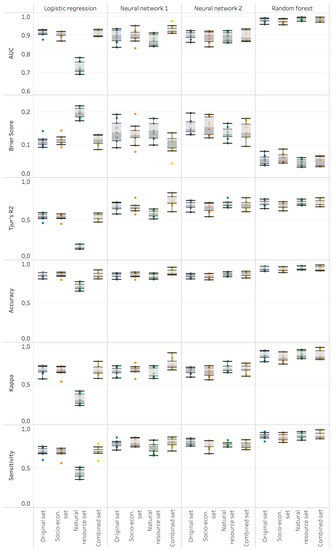
Figure 1.
Model performance according to area under curve (AUC), Brier score, Tjur’s R2, overall accuracy, Kappa index of agreement and sensitivity calculated on 10 iterations of test data sets for all 16 models, i.e., four variable sets using four modelling approaches. Note: the y-scales are different for the six metrics.
Contrary to our expectations, the addition of natural resource variables does not substantially improve the performance of conflict risk models (Figure 1). All six performance metrics demonstrate this evidence consistently. Figure 1 shows that the models based on the dataset combining socio-economic and natural resource variables perform similar as models trained on the original dataset when applying logistic regression and random forest. The combined dataset model performs slightly better than the original when applying both neural networks. Models based on only natural resource variables perform much worse when applying logistic regression, slightly worse in the neural networks, but slightly better when applying random forest compared to all other variable sets (Figure 1). Lastly, the models trained on only socio-economic variables tend to perform slightly worse than the models based on the original dataset for the logistic regression and the random forest models, but similar for the neural networks (Figure 1).
The highest overfitting is found in the combined dataset model that applies neural network 2 (ΔAUC = 0.08). The other neural networks are slightly overfitted (ΔAUC ≈ 0.04). The random forest and logistic regression models practically were not overfitted (ΔAUC ≤ 0.02). These patterns can be explained technically, rather than content-wise: neural networks have the tendency to overfit, especially when trained on large datasets such as the combined set. Random forest models on the other hand were developed with the specific goal of addressing overfitting issues of other machine learning techniques. Concerning model stability, the logistic regression model based on only natural resource variables is less stable than the logistic models based on the other three variable sets, consistently over all six performance metrics (Figure 1). Otherwise, the stability of the 16 models do not demonstrate any specific pattern related to the variable sets. Generally, the random forest models are most stable, while the neural networks perform the least stable.
3.2. Variable Importance and Interactions
Natural resource variables stand high in the predictor importance hierarchy (Figure 2). Recent internal conflict is noticeably the most important predictor in the three variable sets that contain socio-economic data, with the highest accuracy decrease and lowest mean minimal depth. Concerning natural resources, population size and food security are among the 10 most important predictors in the original dataset. In the natural resource set and combined set, population density, food security, water access, and forest area are among the 10 most important predictors. Arable land is important too with similar accuracy decrease and mean minimal depth as population density, but present in less nodes. Fuel export, ore export and resource rent occur in all models among the least important half of all predictors. Water stress is only among the eight least important of 24 predictors in the original dataset. However, when replacing the low-quality water stress variable with better water-related variables in the new natural resource set (Table 1), water access is among the top 10 predictors (Figure 2). In the three models including socio-economic data, i.e., based on the original dataset, on the socio-economic dataset, and on the combined dataset, the socio-economic variables among the top 10 predictors are: recent internal conflict, level of repression, infant mortality, GDP per capita, government effectiveness, and youth bulge.
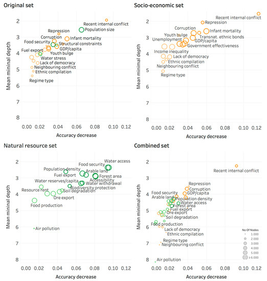
Figure 2.
Variable importance plots of the four random forest models, i.e., trained on the four variable sets. Per model, we plotted for each variable: the MSE accuracy decrease, the mean minimal depth, and the number of nodes using that specific variable for splitting, respectively on the x-axis, y-axis, and by the size of the data point. Important variables have a high accuracy decrease, a low mean minimal depth, and high number of nodes, and thus are plotted towards the upper right corner as large data points. Orange indicates socio-economic predictors; green indicates natural resource predictors. The 10 most important predictors are tinted darker, based on a joined ranking of the three importance metrics presented.
To better interpret the importance and interaction plots (Figure 2 and Figure 3), the conditional and unconditional depths of variable interactions can be compared with the average size of decision trees in the random forest models (Table 2). In general, the 10 closest variable interactions per model all have mean conditional depths lower than 4.1 (Figure 3). In other words, those 10 most closely interacting variables are on average closer than 4 four from each other in all the decision trees of the random forest. In comparison to the average tree size and forest structure (Table 2), this can be considered a close positioning of those two variables and thus a relevant potential interaction between them. In technical terms, those 10 pairs of most closely interacting variables per model are on average positioned closer to each other in the decision tree structures than half of the average tree size (depth) or than a quarter of the maximum tree size (Table 2). Remember that only a random subsample of all predictor variables is considered at each split in a decision tree. This means that two closely interacting predictors will never occur in two splits right beside each other in all 500 trees of the random forest. Thus, a distance between two interacting variables, i.e., conditional depth, of 1 or smaller is impossible. Consequently, we can interpret a mean conditional depth lower than 4.1 (Figure 3) as a close interaction compared to the average size of the decision trees in the random forest models (Table 2).
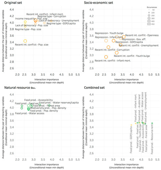
Figure 3.
Variable interaction plots of the four random forest models, i.e., trained on the four variable sets. Per model, we plotted for each variable interaction: the conditional mean minimal depth, the unconditional mean minimal depth, and the frequency of occurrences, respectively on the y-axis, x-axis, and by the size of the data point. Thus, large data points in the lower left corner indicate close and important interactions. Only the 10 closest interactions are presented per model. Orange indicates interactions between socio-economic variables, yellow between socio-economic and natural resource variables, and green between only natural resource variables.
Table 2.
Overview of the size of decision trees in each of the four random forest models, i.e., trained on the four variable sets. Tree depth means the number of splits from root to terminal node of a decision tree.
In the original variable set, population size is the most interacting variable (Figure 3). It interacts with recent internal conflict, regime type, lack of democracy, and income inequality, in increasing order of conditional depth (Figure 3). The other main interactions for this model are purely socio-economic with regime type and infant mortality present in four and three interactions respectively out of the top 10 interactions. The interaction of recent internal conflict with population size is clearly the closest and most important with an average distance (conditional mean minimal depth) of 3.4 between them; an unconditional mean minimal depth of 2.5; and 420 occurrences over 500 trees.
The socio-economic based model overall shows the closest and most frequent interactions for predicting conflict risk (Figure 3). The strongest interactions occur between recent internal conflict and infant mortality, youth bulge, or corruption. The second root variable occurring in the top 10 interactions of this model is repression, interacting with GDP per capita, infant mortality, government effectiveness, and youth bulge.
The top 10 interactions of the natural resource set show a similar closeness and importance as the model based on the original dataset, i.e., average distances between interacting variables (conditional mean minimal depths) of around 4 and unconditional mean minimal depths around between 2.3 and 4 (Figure 3). Two interactions, food production–water access and food production–food security, have the highest importance in predicting (lowest unconditional mean minimal depths) of all interactions present within the four models.
The top 10 interactions of the combined set, with conditional minimal depths smaller than 3.6, are all closer than the original set’s interactions (Figure 3). The closest interaction is Food production–GDP per capita with an importance (unconditional depth) below 4. All other of the top 10 interactions have Food production as a root variable too, combined with socio-economic variables such as infant mortality, youth bulge, or unemployment; as well as with natural resource variables such as food security, water access, accessibility, forest area, and resource rent. All the interactions within the combined set have relatively low number of occurrences: on average each of the top 10 interactions occurs 84 times among the 500 trees of the forest.
4. Discussion
4.1. Seemingly Conflicting Role of Natural Resources
Our findings convey two seemingly conflicting messages: (1) adding natural resource variables does not substantially improve conflict risk predictions, and (2) natural resources stand high in the predictor importance hierarchy. Yet, we see compatibility. We interpret that signals from natural resources leading to conflict risk are reflected in and influenced by socio-economic conditions. In other words, we infer that natural resources are one of several root causes leading to violent conflict, mediated by their socio-economic and political context. We base this interpretation on the following four considerations from this study’s empirical results, in light of the existing literature discussed below in Section 4.2.
First, no strong direct relation was found between only natural resource variables and risk for violent conflict: Figure 1 shows a weak predictive performance of the logistic regression based on the natural resource set. This has been shown by various peace and conflict scholars before, e.g., [21,91]. However, their effect on conflict risk may be indirect, as supported by many researchers, e.g., [17]. Second, socio-economic conditions alone are strong conflict predictors when linked directly in logistic regression models without complex interactions (Figure 1). They can potentially incorporate effects from natural resources, such as water access for example influences child mortality [92]. Third, the models with only natural resource variables are able to predict conflict risk very well when using more complex models (Figure 1). We interpret that complex-systems-based methods can recreate the indirect effects of natural resources on socio-economic drivers that can directly predict conflict risk, based on only natural resource variables. The complex-systems-based models based on only natural resource variables seem to be able to capture the indirect, mediating signal of socio-economic drivers. Lastly, the overall high predictive performance of the machine learning approaches prevents us from detecting substantial improvements by adding or removing natural resource variables (Figure 1). Likewise, the inclusion of variables capturing autocorrelation such as recent internal conflict in the models based on the original, socio-economic, and combined datasets improve the predictive performance very much (Figure 2), leaving less room for improvement when including or excluding natural resource variables.
While it is not necessary to include natural resource variables in purely predictive models on the short term, precious conflict prevention time can be gained by considering natural resources in predicting conflicts. Including natural resources is also imperative in models that aim to investigate the root causes of violent conflicts, either for research or policy-making on conflict prevention. The following sub-section will attempt to clarify plausible causal pathways from natural resources to violent conflicts by building on our importance and interaction analysis of natural resources variables and comparing it with existing literature.
4.2. Natural Resources Are Important, Interacting Predictors
The natural resource-related variables with important roles as predictors were Population size and density, Food security, Water access, Forest area, and Arable land. The natural resource variable most closely interacting with other variables was Food production.
4.2.1. Population
Our results show that population size and density are important predictors of conflict risk in models that allow for complex variable interactions (Figure 2). There is consensus among the majority of studies that population growth or a high population density alone does not directly lead to violent conflict [93,94,95]. Indirect effects of population changes on violent conflict are supported in the literature. On the one hand, population growth leads to environmental degradation and increased resource scarcity, which can reduce agricultural and economic productivity [94,95]. On the other hand, unequal population growth or migration changes the local balance between religious, ethnic, linguistic, or class groups [94,95]. Competition over scarcer resources due to population changes is said to increase the risk for internal violent conflict if the following two conditions co-occur: (1) reduced agricultural or economic productivity, and (2) social stratification [93,94,95]. In Figure 3, we identified the interaction between population density and food production as the closest one of the model based on natural resource variables, as well as the interaction between population size and income inequality as an important one for predicting violent conflict in the model based on the original dataset. Those two identified interactions support such an argument about reduced productivity and social stratification. Yet we identified closer interactions between population and style of governance, i.e., regime type and lack of democracy. We did not find an explanatory hypothesis in the literature that links population to violent conflict through intervening governance factors. Lastly, there is some evidence that large populations increase the risk for armed conflict because of a higher probability of different cultural groups within one country and more opportunities for the mobilization of opposition [95].
4.2.2. Food
The effects of food security and arable land on violent conflict follows three different causal pathways within scientific literature. First, risk of violent conflict has been said to increase with higher food prices in urban areas, prolonged food insecurity in rural areas, severe volatility in food prices, and rapid food shortages [19,20]. Food security, in our analysis, encompasses food price, volatility, and nourishment aspects (Table 1). Because food security is an important predictor variable in our models (Figure 2), our results agree with these earlier findings. Secondly, cropland has been shown to support violent conflict because food is a valuable and lootable resource that can feed and pay combatants [96,97]. Note that this argument only applies to already conflictual situations, with cropland making these conflicts more violent. Even though arable land surfaced as an important predictor (Figure 2), our analysis cannot distinguish between different intensities of violence because of a binary outcome variable. Thirdly, several researchers found no consistent relation between agricultural output and violent conflict [19,21,22]. They argue that the socio-economic and political context is more important than agricultural productivity to understand conflict risk. Hendrix and Brinkman [19] (p. 13) explain that socio-economic and political context "can either mitigate or amplify the effects of food insecurity on conflict”. Based on our results, we only partly agree with these statements. In agreement with Buhaug et al.’s [21] results, food production is not an important predictor in our random forest models (Figure 2). Still, of all the natural resource variables, it is the one that interacts most with other variables (Figure 3). Our findings specified that food production interacts more with economic indicators (GDP per capita and unemployment) and demographic indicators (infant mortality and youth bulge) than with political variables (Figure 3). Therefore, we support the findings of Hendrix and Brinkman [19], Buhaug et al. [21], and Jones, Mattiacci, and Braumoeller [22] that food production is important within its socio-economic context, but not as much within its political context.
4.2.3. Water
The newly added water variables (water access, water reserves/capita, and water withdrawal) are relatively important predictors for the two models with the new natural resource variables, which indicates that water indeed affects conflict risk. The water stress variable of the original dataset can be considered of low quality with little variation in values over the studied period [67,68], which probably explains its low predictive importance. Water seems the most studied natural resource in relation to violent conflict, including droughts, precipitation, and shared international river systems. This is probably because of an intuitive recognition that water is essential to human life [98]. We only discuss a handful of water-conflict studies in relation to our results, covering the main arguments made within the wider water security literature.
Even though many studies start from the hypothesis that water scarcity leads to violent conflict, most studies do not conclude this after their empirical analyses. In a large-scale survey by Marcantonio, Attari, and Evans [28] (p. 14) in sub-Saharan Africa, respondents did "not think water scarcity is a direct source of conflict”, compared to other causes such as land grabbing, crop damage, and politics. Link, Scheffran, and Ide [26] (p. 510) concluded from their review that "despite the fundamental differences in water stress in the various parts of the world, the actual allocation of water is rarely at the heart of the conflict”. Accompanying political and cultural considerations, such as electricity production, hegemonic status, water quality standards, preservation, water service distribution, adaptive capacity of societies, and upstream vs. downstream users, are important steps in the causal pathways from water to violent struggles [24,26,27]. Selby and Hoffmann [25] (p. 1010) even go as far to state that their case studies of Cyprus and Israel–Palestine "provide negligible support for the Malthusian thesis that water scarcity can cause or contribute to conflict and migration”. Further, Gizelis, and Wooden [23] and Adano et al. [99], in an empirical large-n study and a Kenya case study found that water abundance, rather than water scarcity, leads to violent conflict. What is distinct about the water scarcity literature, compared to other natural resource scarcities, is the argument that water scarcity or degradation could also lead to cooperation instead of conflict. Most of the literature points to a significant role for institutions, be they traditional or official, to mediate how water resources influence violent conflict or cooperation [23,27,99,100].
Our analysis disagrees with most findings by the researchers mentioned above. Water access is among the top 10 predictors for violent conflict risk in the random forest models that include the new natural resource variables. Water reserves per capita and water withdrawal are the 13th and 14th most important predictors of 35 variables in the combined set, following the top 10 closely. Moreover, our results do not identify any close socio-economic interaction with one of the water variables to predict conflict risk, and thus indicate that water access, reserves and withdrawal are important factors independent of mediating socio-economic effects. The only important interaction found is with food production, which is a logical biophysical relation.
4.2.4. Forest
Although less studied than other natural resources, forest area is among the important natural resource predictors for conflict risk (Figure 2). Researchers have described three distinct links between forest area and violent conflict. First, rich forests are generally located far from mainstream commercial activity and government control [29]. Communities living in forests are often marginalised geographically, politically, and socially, as well as economically [29]. Development and implementation of property rights are often lacking, inadequate, or discriminatory [29]. Competition over the forests’ rich resources between disadvantaged groups, in combination with weak institutions, promotes violent conflict in forested areas [30,31]. Secondly, scarcity of forest land has been perceived as a direct cause for relapse into violent conflict only in a post-war setting, after contested redistributions of forest land [101,102]. Thirdly, even when forests are not among the initial causes of conflicts, they tend to become involved because of the specific goods and services they provide [29]. Forests provide marketable materials to finance conflicts, such as timber, wildlife, medicinal plants, and hidden land for the cultivation of illegal drug crops. Rivalry over access to and control over these goods turns forest lands into strategic resources [29]. Moreover, forests function as venues for violent conflicts because of the shelter they provide to civilians and refugees, as well as guerrilla-style militia [32]. According to our interaction analysis, forest area only interacts with food production (Figure 3). This finding does not support nor is it in disagreement with any of the causal paths suggested in the literature.
4.2.5. Ores and Oil
Surprisingly, ore and metals exports, oil export, and resource rent are not as important for predicting conflict risk than the natural resource variables described above (Figure 2). This is an interesting finding with respect to the seminal studies on the resource curse. Collier and Hoeffler’s [5] econometric analysis shows that natural resource extraction significantly increases conflict risk. They explain that finances from resource exports make rebellion feasible and attractive. Additionally, they argue that a strong dependence on primary commodities worsens governance and so generates strong grievances. Le Billon [6] comes to the same conclusions as Collier and Hoeffler [5] through several in-depth case studies: resources and wars are linked because resource revenues finance rebellions, resource exploitation generates tension, and resource dependence presents major governmental challenges. Our analysis does not contest these findings, but indicates that non-renewable resource variables, which are related rather to abundance theories of conflict risk [18], are less important for predicting intrastate violent conflict than renewable resource variables, such as food security, water access, forest area, and arable land, which have been more related to resource scarcity theories of conflict risk [18].
4.2.6. Socio-Economic vs. Natural Resource Variables
The discussion above demonstrates that natural resources variables are important to predict conflict risk. Still, they are less important than the following socio-economic variables: recent internal conflict, level of repression, infant mortality, GDP per capita, and government effectiveness (Figure 2). Youth bulge is of similar importance as most natural resource variables, while other common predictors, such as regime type, neighbouring conflict, ethnic compilation, lack of democracy, and empowerment rights are less important than the discussed natural resource variables. Additionally, the 10 closest interactions in the combined model and the four most important interactions in the original model all include at least one natural resource variable (Figure 3). For these reasons, and following the discussion paragraphs above, we interpret that scarcity, as well as abundance of natural resources, can drive violent conflict as root causes moderated by socio-economic or political contexts. Current globally unsustainable trends, such as deforestation, increased consumption, population growth, and climate change, are projected to increasingly impact the natural resource base [9]. Through natural resources, we infer that these trends are contributing and will continue to contribute to violent conflicts worldwide. To achieve sustainable peace, we deem it necessary to include natural resources in explanatory research and decision-making on conflict prevention.
4.2.7. Limitations
There are some limitations to the quality of data used in the analysis. Water stress and soil degradation miss many observations and do not change much per country over the studied years. This probably explains their low importance for predicting conflict risk. Both water stress and soil degradation relate biophysically to arable land, food production, and eventually food security, which are all important predictors. Therefore, we expect that, with better data, soil degradation would be a more important predictor or interact more closely with other food related variables, similar to the new water variables (Figure 2 and Table 1). Further, we can improve the causal analysis by increasing the country-year resolution of the studied data [103]. More and more conflict data are becoming globally available on sub-national statistical units, even on a grid scale of 0.5° by 0.5°, and at monthly time slices [104]. We dealt with the auto-correlation through time and space of the conflict data in country-year units by including the variables recent internal conflict, years since highly violent conflict, and neighbouring conflict. Another possible way to reduce the effects of autocorrelation on prediction and analysis results is by working with events-based data. This means every conflict is one observation in the dataset, even if it crosses years and political boundaries. Then the role of natural resources can be studied in terms of the onset, duration and end of violent conflicts. Difficulties with this approach would be to delineate one conflict observation, i.e., when do different violent actions belong to one and the same conflict observation and when are they part of different conflicts. This is because conflicts have spill-over effects creating new grievances, new militia, and new conflicts [105]. Hence, it remains difficult to separate between different conflict observations and to completely cancel out spatial and temporal autoregression.
Model development, for logistic regression as well as machine learning methods, is an iterative process. Variable selection for the optimal predictive model should be a stepwise process in including necessary, or excluding superfluous, variables. Furthermore, the model structure of neural networks and random forests can be optimised. It was not our aim to create the best predictive models, but to investigate the relevance of adding natural resource variables to complexity-based conflict models. Towards that aim, standard settings for model structure suffice. Superfluous variables were identified as less important, without influencing the analysis of the role of other variables towards predicting conflict risk too much. Examples of such unimportant, uninfluential variables were biodiversity conservation and renewable energy production (Figure 2). We chose a large standard number of decision trees within the random forests to be able to detect frequently occurring interactions.
Currently, methods and tools for interpretation of machine learning and predictive models are being continuously developed, tested, and improved, e.g., [65]. We applied variable importance and interaction metrics specifically developed specifically for random forest models [87]. More and more importance and interaction metrics are being developed that can be applied to many different types of prediction models [106]. In this paper, such model-agnostic metrics could be applied to and compared between the logistic regression, neural networks and random forest. The advantages of such model-agnostic tools are that the role of variables can be interpreted and compared between different types of models. Permutation accuracy decrease, as used in the above analysis, is one of those and can be extended to the logistic regression and neural network provided many extra coding efforts [65]. The other variable importance and interactions metrics, i.e., mean minimal depth, number of nodes, and conditional mean minimal depth, are only applicable to random forest models and could be replaced by model-agnostic tools currently being developed.
Even though complex computational models, such as neural networks and random forests, are able to incorporate nonlinearities and interactions between variables, these empirically based methods have their limits. They only learn from observations recorded within a limited time span, in this case 1989 to 2014 [51]. The statistical metrics are not able to distinguish between root variables and mediating variables and to test plausible indirect causal pathways, which is why these needed to be interpreted form the data-driven results of this paper and existing literature. Data-driven approaches more easily neglect existing causal theories, as well as avoid contributing to new theory [51]. Other complex system methods, such as system dynamics modelling, agent-based modelling, network analysis, and scenario development, can complement complex empirical models to study the natural resources–violent conflict link. These methods provide greater freedom of choice between an empirical or theoretical grounding to analyse complex systems.
5. Conclusions
This study found that natural resource variables are important predictors of conflict, though we interpret their effects to be often captured by the intervening socio-economic variables. Adding natural resource variables does not substantially increase the performance of conflict risk models, even when allowing for nonlinearities and complex interactions through machine learning. Nevertheless, several natural resources ranked among the top 10 of important predictor variables, including population density, food security, water access, forest area, and arable land. The closest natural resource–society interaction to predict conflict risk according to our models was food production within its economic and demographic context, e.g., with GDP per capita, unemployment, infant mortality and youth bulge. The results demonstrated that resource rents, oil export, ore and metal export are less important predictors relative to the natural resource variables mentioned above than prior research has suggested.
From our analysis, we interpreted, in light of the existing literature, that natural resources can be among the root causes of violent conflict, moderated within their socio-economic or political context. We inferred that natural resource signals to conflict risk are indirect, with probably several mediating socio-economic and political steps in the causal pathway from natural resources to violent conflict. If so, precious conflict prevention time and strategies can be gained by considering natural resources. In consequence, we consider it important to include natural resources in models that can account for complex interactions if the purpose is to investigate root causes of and complex causal pathways to violent conflicts, either for research or policy-making on conflict prevention. We consider that sustainable peace requires sustainable and conflict-sensitive resource use and management. This is even more imperative because of ongoing and projected trends that affect natural resources, such as deforestation, increased consumption, biodiversity loss, and climate change. However, it is not necessary to include natural resource variables in purely short-term predictive models used as conflict early warning systems.
Many research opportunities follow from this analysis. First, we recommend that researchers harness the full, also explanatory, power of complex computational tools to understand drivers of violent conflicts. The variable analysis within predictive models can be deepened by extracting and visualising the direction of the effects of certain important variables—positive or negative—on conflict risk and also in consideration of the interaction with other variables. Furthermore, it would be possible to investigate three-step interactions instead of only two-variable interactions. Preferably, model-agnostic interpretation methods would be used. Secondly, we mentioned possible model improvements by including better data for the soil variable, the use of higher-resolution data spatially and temporally rather than country-year observations, the use of conflict-event data, stepwise variable selection, and optimisation of the neural network and random forest structures. Lastly, we are searching for statistical metrics to distinguish root causes from mediating variables and to test plausible indirect causal pathways. While investigating the former, we recommend the use of other complex system methods, as well as qualitative theoretical studies, to complement these empirical findings with more theory driven approaches on the complex link between natural resources and the risk for violent conflict.
Supplementary Materials
The following are available online at https://www.mdpi.com/2071-1050/12/16/6574/s1: data for the natural resource variables, and codebook for development of neural networks, random forest models, model performance comparison, and variable importance and interaction analysis.
Author Contributions
Conceptualization, M.K.S.; data curation, M.K.S.; formal analysis, M.K.S.; investigation, M.K.S.; methodology, M.K.S.; supervision, S.B.; validation, M.K.S. and S.B.; visualization, M.K.S; writing—original draft preparation, M.K.S.; writing—review and editing, S.B. and M.K.S. All authors have read and agreed to the published version of the manuscript.
Funding
This research was funded by the European Union’s Horizon 2020 research and innovation programme under the Marie Skłodowska-Curie Innovative Training Network, grant number 675153.
Acknowledgments
We would like to thank the Peace and Conflict team at the EC JRC who supported us in working with the Global Conflict Risk Index. We are also grateful to John Miller and Scott Page from the Santa Fe Institute who helped us develop questions and tools to analyse conflicts computationally as complex social phenomena. Lastly, we are grateful to Maartje Oostdijk and several anonymous reviewers who improved this manuscript with their constructive feedback.
Conflicts of Interest
The authors declare no conflict of interest. The funders had no role in the design of the study; in the collection, analyses, or interpretation of data; in the writing of the manuscript, or in the decision to publish the results.
Appendix A
Table A1.
Overview of metrics calculated to compare the models’ performances.
Table A1.
Overview of metrics calculated to compare the models’ performances.
| Performance Metric | Calculation | Motivation/Advantages | Source | Key for Interpretation |
|---|---|---|---|---|
| Calculated directly from predicted probabilities * | ||||
| Area Under Curve (AUC) | Area under the receiver operating characteristic (ROC) curve. The ROC curve plots the sensitivity against fall out rate (see further down in this table) over the whole range of possible classification thresholds (0 to 1) | Commonly used to assess how well a model discriminates between high-risk and low-risk subjects. High sensitivity combined with low fall out rates over the whole range of thresholds leads to a larger area under the ROC curve. | [86,107] | Between 0.5 and 1. The higher, the better. |
| Brier score | The average of the squared prediction error, similar to the Mean Squared Error (MSE) for linear regression. It evaluates the calibration of the model while all other measures evaluate the discrimination by the model. | [107,108] | It generally ranges from 0 (perfect) to 0.25 (worthless). It is the only measure in this analysis for which holds the lower the better. | |
| Tjur’s R2 | Coefficient of discrimination, a highly recommended R2-substitute for logistic regression models. It calculates the difference between the averages of predicted values for 1 and 0 observations, respectively. Its ease of interpretation comes from the fact it uses terms and concepts that are directly related to models for binary observations on their own premises, without any reference to variance and variation concepts. On top, it has close direct mathematical relations with the standard formulas of R2. | [109] | Between 0 and 1, the higher the better. | |
| Calculated from predictions classified into “no conflict risk” vs. “conflict risk”, based on based on a probability threshold of 0.5 ** | ||||
| Overall accuracy | Proportion correctly predicted, easy to understand. The large amount of easy to predict peace events makes this performance measure less useful. | As a percentage or ratio. The closer to one the better. | ||
| Kappa index of agreement (Cohen’s kappa) | with expected accuracy and | The amount of observed accuracy corrected by the accuracy expected by chance. With unbalanced data, there is a higher chance you will randomly classify the less common group so this should be and is accounted for in kappa. | [110] | Can range from −1 to +1. Suggested guidelines by [110]: < or = 0: no agreement 0.01–0.20: non to slight 0.21–0.40: fair 0.41–0.60: moderate 0.61–0.80: substantial 0.81–1.00: almost perfect agreement |
| Sensitivity (hit rate, recall, true positive rate) | The chance that a conflict event will be predicted, probability of detection, the percentage of conflict events which are classified as such. Slightly more difficult to understand than overall accuracy, but more relevant in a rare event context, such as violent conflicts. | As a percentage or ratio. The closer to 1 the better. | ||
* y denotes the observed outcome and p the prediction for subject i in a dataset of n subjects; and denote respectively the averages of predicted values for observed 1-values (i.e., observed conflict risk) and 0-values (i.e., no observed conflict risk). ** TN = True Negative, TP = True Positive, FN = False Negative (Type II error), FP (Type I error).
References
- UN General Assembly Transforming Our World: The 2030 Agenda for Sustainable Development; United Nations: New York, NY, USA, 2015; Code A/RES/70/1; p. 35.
- Homer-Dixon, T.F. Environmental Scarcities and Violent Conflict: Evidence from Cases. Int. Secur. 1994, 19, 5. [Google Scholar] [CrossRef]
- Sachs, J.D.; Warner, A.M. The curse of natural resources. Eur. Econ. Rev. 2001, 45, 827–838. [Google Scholar] [CrossRef]
- Lujala, P. The spoils of nature: Armed civil conflict and rebel access to natural resources. J. Peace Res. 2010, 47, 15–28. [Google Scholar] [CrossRef]
- Collier, P.; Hoeffler, A. Greed and Grievance in Civil War. Oxf. Econ. Pap. 2004, 56, 563–595. [Google Scholar] [CrossRef]
- Le Billon, P. Wars of Plunder: Conflicts, Profits and the Politics of Resources; Hurst & Company Ltd.: London, UK, 2012; ISBN 978-1-84904-145-4. [Google Scholar]
- Krausmann, F.; Erb, K.-H.; Gingrich, S.; Haberl, H.; Bondeau, A.; Gaube, V.; Lauk, C.; Plutzar, C.; Searchinger, T.D. Global human appropriation of net primary production doubled in the 20th century. Proc. Natl. Acad. Sci. USA 2013, 110, 10324. [Google Scholar] [CrossRef] [PubMed]
- IPCC. Climate Change 2014: Synthesis Report. Contribution of Working Groups I, II and III to the Fifth Assessment Report of the Intergovernmental Panel on Climate Change; Intergovernmental Panel on Climate Change: Geneva, Switzerland, 2014; p. 151. [Google Scholar]
- UNEP. Global Environment Outlook 6: Healthy Planet, Healthy People; Ekins, P., Gupta, J., Boileau, P., Eds.; Cambridge University Press: New York, NY, USA, 2019; ISBN 978-1-108-70766-4. [Google Scholar]
- Barnett, J.; Adger, N. Environmental Change, Human Security, and Violent Conflict. In Global Environmental Change and Human Security; Matthew, R.A., Ed.; MIT Press: Cambridge, MA, USA, 2010; ISBN 978-0-262-01340-6. [Google Scholar]
- Klare, M. The Race for What’s Left: The Global Scramble for the World’s Last Resources; Macmillan: New York, NY, USA, 2012; ISBN 978-1-4299-7330-4. [Google Scholar]
- UNFT. EU-UN Partnership on Land, Natural Resources and Conflict Prevention: Introduction and Overview; UN Interagency Framework Team for Preventive Action (UNFT): New York, NY, USA, 2011. [Google Scholar]
- From Conflict to Peacebuilding: The Role of Natural Resources and the Environment; UNEP, Ed.; Policy Paper; United Nations Environment Programme: Nairobi, Kenya, 2009; ISBN 978-92-807-2957-3. [Google Scholar]
- Adger, W.N.; Pulhin, J.M.; Barnett, J.; Dalbeko, G.D.; Hovelsrud, G.K.; Levy, M.; Oswald Spring, Ú.; Vogel, C.H. Human Security. In Climate Change 2014: Impacts, Adaptation, and Vulnerability. Part A: Global and Sectoral Aspects. Contribution of Working Group II to the Fifth Assessment Report of the Intergovernmental Panel on Climate Change; Field, C.B., Barros, V.R., Dokken, D.J., Mach, K.J., Mastrandrea, M.D., Billir, T.E., Chatterjee, M., Ebi, K.L., Estrada, Y.O., Genova, R.C., et al., Eds.; Cambridge University Press: Cambridge, UK; New York, NY, USA, 2014; pp. 755–791. [Google Scholar]
- IPCC. Climate Change 2007: Impacts, Adaptations and Vulnerability. Contribution of Working Group II to the Fourth Assessment Report of the Intergovernmental Panel on Climate Change; Parry, M.L., Palutikof, J.P., van der Linden, P.J., Hanson, C.E., Eds.; Cambridge University Press: Cambridge, UK, 2007; ISBN 978-0-521-88009-1. [Google Scholar]
- General Secretariat of the Council. Council Conclusions on Climate Diplomacy; Council of the European Union: Brussels, Belgium, 2018. [Google Scholar]
- Mildner, S.-A.; Lauster, G.; Wodni, W. Scarcity and Abundance Revisited: A Literature Review on Natural Resources and Conflict. Int. J. Confl. Violence 2011, 5, 155–172. [Google Scholar]
- Koubi, V.; Spilker, G.; Böhmelt, T.; Bernauer, T. Do natural resources matter for interstate and intrastate armed conflict? J. Peace Res. 2014, 51, 227–243. [Google Scholar] [CrossRef]
- Hendrix, C.; Brinkman, H.-J. Food Insecurity and Conflict Dynamics: Causal Linkages and Complex Feedbacks. Stab. Int. J. Secur. Dev. 2013, 2, Art. 26. [Google Scholar] [CrossRef]
- Brück, T.; d’Errico, M. Food security and violent conflict: Introduction to the special issue. World Dev. 2019, 117, 167–171. [Google Scholar] [CrossRef]
- Buhaug, H.; Benjaminsen, T.A.; Sjaastad, E.; Theisen, O.M. Climate variability, food production shocks, and violent conflict in Sub-Saharan Africa. Environ. Res. Lett. 2015, 10, 125015. [Google Scholar] [CrossRef]
- Jones, B.T.; Mattiacci, E.; Braumoeller, B.F. Food scarcity and state vulnerability: Unpacking the link between climate variability and violent unrest. J. Peace Res. 2017, 54, 335–350. [Google Scholar] [CrossRef]
- Gizelis, T.-I.; Wooden, A.E. Water resources, institutions, & intrastate conflict. Polit. Geogr. 2010, 29, 444–453. [Google Scholar] [CrossRef]
- Brochmann, M.; Gleditsch, N.P. Shared rivers and conflict—A reconsideration. Polit. Geogr. 2012, 31, 519–527. [Google Scholar] [CrossRef]
- Selby, J.; Hoffmann, C. Water scarcity, conflict, and migration: A comparative analysis and reappraisal. Environ. Plan. C Gov. Policy 2012, 30, 997–1014. [Google Scholar] [CrossRef]
- Link, P.M.; Scheffran, J.; Ide, T. Conflict and cooperation in the water-security nexus: A global comparative analysis of river basins under climate change. Wiley Interdiscip. Rev. Water 2016, 3, 495–515. [Google Scholar] [CrossRef]
- Feitelson, E.; Tubi, A. A main driver or an intermediate variable? Climate change, water and security in the Middle East. Glob. Environ. Chang. 2017, 44, 39–48. [Google Scholar] [CrossRef]
- Marcantonio, R.A.; Attari, S.Z.; Evans, T.P. Farmer Perceptions of Conflict Related to Water in Zambia. Sustainability 2018, 10, 313. [Google Scholar] [CrossRef]
- De Jong, W.; Donovan, D.; Abe, K. (Eds.) Extreme Conflict and Tropical Forests; World Forests; Springer: Dordrecht, The Netherlands, 2007; ISBN 978-1-4020-5461-7. [Google Scholar]
- De Koning, R. Greed or Grievance in West Africa’s Forest Wars? In Extreme Conflict and Tropical Forests; De Jong, W., Donovan, D., Abe, K.-I., Eds.; World Forests; Springer: Dordrecht, The Netherlands, 2007; pp. 37–56. ISBN 978-1-4020-5462-4. [Google Scholar]
- Swatuk, L.A. Seeing the Forest for the Trees: Tropical Forests, the State and Violent Conflict in Africa. In Extreme Conflict and Tropical Forests; De Jong, W., Donovan, D., Abe, K.-I., Eds.; World Forests; Springer: Dordrecht, The Netherlands, 2007; pp. 93–115. ISBN 978-1-4020-5462-4. [Google Scholar]
- Donovan, D.; De Jong, W.; Abe, K.-I. Tropical Forests and Extreme Conflict. In Extreme Conflict and Tropical Forests; Jong, W.D., Donovan, D., Abe, K.-I., Eds.; World Forests; Springer: Dordrecht, The Netherlands, 2007; pp. 1–15. ISBN 978-1-4020-5462-4. [Google Scholar]
- Ward, M.D.; Metternich, N.W.; Dorff, C.L.; Gallop, M.; Hollenbach, F.M.; Schultz, A.; Weschle, S. Learning from the Past and Stepping into the Future: Toward a New Generation of Conflict Prediction. Int. Stud. Rev. 2013, 15, 473–490. [Google Scholar] [CrossRef]
- Schrodt, P.A.; Yonamine, J.; Bagozzi, B.E. Data-based Computational Approaches to Forecasting Political Violence. In Handbook of Computational Approaches to Counterterrorism; Subrahmanian, V.S., Ed.; Springer: New York, NY, USA, 2013; pp. 129–163. ISBN 978-1-4614-5310-9. [Google Scholar]
- Gleditsch, K.S.; Ward, M.D. Forecasting is difficult, especially about the future: Using contentious issues to forecast interstate disputes. J. Peace Res. 2013, 50, 17–31. [Google Scholar] [CrossRef]
- Goldstone, J.A.; Bates, R.H.; Epstein, D.L.; Gurr, T.R.; Lustik, M.B.; Marshall, M.G.; Ulfelder, J.; Woodward, M. A Global Model for Forecasting Political Instability. Am. J. Polit. Sci. 2010, 54, 190–208. [Google Scholar] [CrossRef]
- Hegre, H.; Karlsen, J.; Nygård, H.M.; Strand, H.; Urdal, H. Predicting Armed Conflict, 2010–2050. Int. Stud. Q. 2013, 57, 250–270. [Google Scholar] [CrossRef]
- Ward, M.D.; Beger, A. Lessons from near real-time forecasting of irregular leadership changes. J. Peace Res. 2017, 54, 141–156. [Google Scholar] [CrossRef]
- Guo, W.; Gleditsch, K.; Wilson, A. Retool AI to forecast and limit wars. Nature 2018, 562, 331–333. [Google Scholar] [CrossRef] [PubMed]
- Beck, N.; King, G.; Zeng, L. Improving Quantitative Studies of International Conflict: A Conjecture. Am. Polit. Sci. Rev. 2000, 94, 21–35. [Google Scholar] [CrossRef]
- Perry, C. Machine Learning and Conflict Prediction: A Use Case. Stab. Int. J. Secur. Dev. 2013, 2, 56. [Google Scholar] [CrossRef]
- Muchlinski, D.; Siroky, D.; He, J.; Kocher, M. Comparing Random Forest with Logistic Regression for Predicting Class-Imbalanced Civil War Onset Data. Polit. Anal. 2016, 24, 87–103. [Google Scholar] [CrossRef]
- Grömping, U. Variable Importance Assessment in Regression: Linear Regression versus Random Forest. Am. Stat. 2009, 63, 308–319. [Google Scholar] [CrossRef]
- Strobl, C.; Boulesteix, A.-L.; Kneib, T.; Augustin, T.; Zeileis, A. Conditional variable importance for random forests. BMC Bioinform. 2008, 9, 307. [Google Scholar] [CrossRef]
- Ward, M.D.; Greenhill, B.D.; Bakke, K.M. The perils of policy by p-value: Predicting civil conflicts. J. Peace Res. 2010, 47, 363–375. [Google Scholar] [CrossRef]
- Colaresi, M.; Mahmood, Z. Do the robot: Lessons from machine learning to improve conflict forecasting. J. Peace Res. 2017, 54, 193–214. [Google Scholar] [CrossRef]
- UN Security Council Security Council Pledges Strengthened UN Effectiveness in Preventing Conflict, Including Through Use of Early Warning, Preventive Deployment, Mediation. 6621st Meeting. Available online: https://www.un.org/press/en/2011/sc10392.doc.htm (accessed on 24 August 2018).
- De Groeve, T.; Hachemer, P.; Vernaccini, L. Global Conflict Risk Index: A Quantitative Model—Concept and Methodology; JRC Scientific and Policy Reports; Joint Research Centre: Publications Office of the European Union: Luxembourg, 2014; p. 68. [Google Scholar]
- Halkia, M.; Ferri, S.; Schellens, M.K.; Papazoglou, M.; Thomakos, D. The Global Conflict Risk Index: A quantitative tool for policy support on conflict prevention. Prog. Disaster Sci. 2020, 6, 1–22. [Google Scholar] [CrossRef]
- Celiku, B.; Kraay, A. Predicting Conflict; World Bank Group: Washington, DC, USA, 2017; p. 46. [Google Scholar]
- Cederman, L.-E.; Weidmann, N.B. Predicting armed conflict: Time to adjust our expectations? Science 2017, 355, 474–476. [Google Scholar] [CrossRef] [PubMed]
- Hegre, H.; Buhaug, H.; Calvin, K.V.; Nordkvelle, J.; Waldhoff, S.T.; Gilmore, E. Forecasting civil conflict along the shared socioeconomic pathways. Environ. Res. Lett. 2016, 11. [Google Scholar] [CrossRef]
- Witmer, F.D.; Linke, A.M.; O’Loughlin, J.; Gettelman, A.; Laing, A. Subnational violent conflict forecasts for sub-Saharan Africa, 2015–2065, using climate-sensitive models. J. Peace Res. 2017, 54, 175–192. [Google Scholar] [CrossRef]
- Pettersson, T.; Högbladh, S.; Öberg, M. Organized violence, 1989–2018 and peace agreements. J. Peace Res. 2019, 56, 589–603. [Google Scholar] [CrossRef]
- Schmidhuber, J. Deep learning in neural networks: An overview. Neural Netw. 2015, 61, 85–117. [Google Scholar] [CrossRef]
- Elisseeff, A.; Paugam-Moisy, H. Size of Multilayer Networks for Exact Learning: Analytic Approach. In Advances in Neural Information Processing Systems 9; Mozer, M.C., Jordan, M.I., Petsche, T., Eds.; MIT Press: Cambridge, MA, USA, 1997; pp. 162–168. [Google Scholar]
- Stathakis, D. How many hidden layers and nodes? Int. J. Remote Sens. 2009, 30, 2133–2147. [Google Scholar] [CrossRef]
- Heaton, J. Introduction to Neural Networks with Java; Heaton Research, Inc.: St. Louis, MO, USA, 2008; ISBN 978-1-60439-008-7. [Google Scholar]
- Reed, R.D.; Marks, R.J. Neural Smithing: Supervised Learning in Feedforward Artificial Neural Networks; MIT Press: Cambridge, MA, USA, 1999; ISBN 978-0-262-18190-7. [Google Scholar]
- Masters, T. Practical Neural Network Recipes in C++; Academic Press: Boston, MA, USA, 1993; ISBN 978-0-12-479040-7. [Google Scholar]
- Ho, T.K. Random decision forests. In Proceedings of the 3rd International Conference on Document Analysis & Recognition, Montreal, QC, Canada, 14–16 August 1995; pp. 278–282. [Google Scholar]
- Breiman, L. Random Forests. Mach. Learn. 2001, 45, 5–32. [Google Scholar] [CrossRef]
- Fernandez-Delgado, M.; Cernadas, E.; Barro, S.; Amorim, D. Do we Need Hundreds of Classifiers to Solve Real World Classification Problems? J. Mach. Learn. Res. 2014, 15, 3133–3181. [Google Scholar]
- Ahmad, M.W.; Mourshed, M.; Rezgui, Y. Trees vs Neurons: Comparison between random forest and ANN for high-resolution prediction of building energy consumption. Energy Build. 2017, 147, 77–89. [Google Scholar] [CrossRef]
- Molnar, C. Interpretable Machine Learning. A Guide for Making Black Box Models Explainable; Github: San Francisco, CA, USA, 2019. [Google Scholar]
- Hsu, A. 2016 Environmental Performance Index; Yale University: New Haven, CT, USA, 2016. [Google Scholar]
- Halkia, M.; Ferri, S.; Joubèrt-Boitat, I.; Saporiti, F. Conflict Risk Indicators: Significance and Data Management in the GCRI; JRC Technical Reports; Joint Research Centre: Publications Office of the European Union: Luxembourg, 2017; p. 82. [Google Scholar]
- Ferri, S.; Papazoglou, M. Personal Communication GCRI Modelling; EC Joint Research Centre: Ispra, Italy, 2018. [Google Scholar]
- Center for Systemic Peace Polity IV: Regime Authority Characteristics and Transitions Datasets. Available online: http://www.systemicpeace.org/inscrdata.html (accessed on 16 September 2017).
- World Bank Worldwide Governance Indicators. Available online: https://datacatalog.-worldbank.org/dataset/worldwide-governance-indicators (accessed on 16 September 2017).
- Gib-ney, M.; Cor-nett, L.; Wood, R.; Hasch-ke, P.; Arnon, D.; Pisanò, A.; Barrett, G. The Political Terror Scale 1976–2018. Available online: http://www.politicalterrorscale.org/Data/ (accessed on 16 September 2017).
- Cingranelli, D.L.; Richards, D.L.; Clay, K.C. The CIRI Human Rights Dataset. Available online: http://www.humanrightsdata.com/p/data-documentation.html (accessed on 16 September 2017).
- Vogt, M.; Bormann, N.C.; Rüegger, S.; Cederman, L.E.; Hunziker, P.; Girardin, L. Integrating Data on Ethnicity, Geography, and Conflict: The Ethnic Power Relations Data Set Family. J. Confl. Resolut. 2015, 59, 1327–1342. [Google Scholar] [CrossRef]
- CIDCM. The Minorities at Risk (MAR) Project: Monitoring the Persecution and Mobilization of Ethnic Groups Worldwide. Available online: http://www.mar.umd.edu/ (accessed on 16 September 2017).
- World Bank World Bank Open Data: Free and Open Access to Global Development Data. Available online: https://data.worldbank.org (accessed on 29 September 2017).
- UN DESA World Population Prospects. Available online: https://population.un.org/wpp/Download/Standard/Population/ (accessed on 29 September 2017).
- Solt, F. The Standardized World Income Inequality Database. Soc. Sci. Q. 2016, 97, 1267–1281. [Google Scholar] [CrossRef]
- FAO Food Security Indicators. Available online: http://www.fao.org/economic/ess/ess-fs/ess-fadata/en/#.Xi7c2hNKg1I (accessed on 29 September 2017).
- Gassert, F.; Reig, P.; Luo, T.; Maddocks, A. Aqueduct Country and River Basin Rankings: A Weighted Aggregation of Spatially Distinct Hydrological Indicators; Working paper; World Resources Institute: Washington, DC, USA, 2013; p. 28. [Google Scholar]
- BTI. Transformation Index of the Bertelsmann Stiftung 2016: Codebook for Country Assessments; Bertelsmann Stiftung (BTI): Gütersloh, Germany, 2016; p. 45. [Google Scholar]
- EM-DAT: The Emergency Events Database; CRED, D, Guha-Sapi, D., Eds.; Université Catholique de Louvain (UCL): Brussels, Belgium, 2017. [Google Scholar]
- Bridges, E.M.; Oldeman, L.R. Global Assessment of Human-Induced Soil Degradation. Arid Soil Res. Rehabil. 1999, 13, 319–325. [Google Scholar] [CrossRef]
- Center for International Earth Science Information Network (CIESIN). Natural Resource Management Index (NRMI), 2011 Release; NASA Socioeconomic Data and Applications Center (SEDAC); Columbia University: Palisades, NY, USA, 2011. [Google Scholar]
- Arlot, S.; Celisse, A. A survey of cross-validation procedures for model selection. Stat. Surv. 2010, 4, 40–79. [Google Scholar] [CrossRef]
- Bergmeir, C.; Hyndman, R.J.; Koo, B. A note on the validity of cross-validation for evaluating autoregressive time series prediction. Comput. Stat. Data Anal. 2018, 70–83. [Google Scholar] [CrossRef]
- Giancristofaro, R.A.; Salmaso, L. Model performance analysis and model validation in logistic regression. Statistica 2003, 63, 375–396. [Google Scholar]
- Paluszyńska, A. Understanding Random Forests with Random Forest Explainer. Available online: https://cran.rstudio.com/web/packages/randomForestExplainer/vignettes/randomForestExplainer.html (accessed on 12 January 2019).
- R Core Team. R: A Language and Environment for Statistical Computing; R Foundation for Statistical Computing: Vienna, Austria, 2018. [Google Scholar]
- Guenther, F.; Fritsch, S. Neuralnet: Training of Neural Networks. R J. 2016, 2, 30–39. [Google Scholar] [CrossRef]
- Liaw, A.; Wiener, M. Classification and Regression by randomForest. R News 2002, 2, 18–22. [Google Scholar]
- O’Brochta, W. A meta-analysis of natural resources and conflict. Res. Polit. 2019, 6, 205316801881823. [Google Scholar] [CrossRef]
- Cheng, J.J.; Schuster-Wallace, C.J.; Watt, S.; Newbold, B.K.; Mente, A. An ecological quantification of the relationships between water, sanitation and infant, child, and maternal mortality. Environ. Health Glob. Access Sci. Source 2012, 11, 4. [Google Scholar] [CrossRef]
- Wittek, R. Resource competition and violent conflict: Cross-cultural evidence for a socio-ecological approach. Z. Für Ethnol. 1990, 115, 23–44. [Google Scholar]
- Gleditsch, N.P.; Urdal, H. Ecoviolence? Links Between Population Growth, Environmental Scarcity and Violent Conflict in Thomas Homer-Dixon’s Work. J. Int. Aff. 2002, 56, 283. [Google Scholar]
- Goldstone, J.A. Population and Security: How Demographic Change Can Lead to Violent Conflict. J. Int. Aff. 2002, 56, 3. [Google Scholar]
- Koren, O.; Bagozzi, B.E. Living off the land: The connection between cropland, food security, and violence against civilians. J. Peace Res. 2017, 54, 351–364. [Google Scholar] [CrossRef]
- Koren, O. Food abundance and violent conflict in Africa. Am. J. Agric. Econ. 2018, 100, 981–1006. [Google Scholar] [CrossRef]
- Armstrong, C. Justice and Natural Resources: An Egalitarian Theory; Oxford University Press: Oxford, NY, USA, 2017; ISBN 978-0-19-870272-6. [Google Scholar]
- Adano, W.R.; Dietz, T.; Witsenburg, K.; Zaal, F. Climate change, violent conflict and local institutions in Kenya’s drylands. J. Peace Res. 2012, 49, 65–80. [Google Scholar] [CrossRef]
- Kuzdas, C.; Wiek, A.; Vignola, R.; Warner, B.; Yglesias, M.; Ramírez-Cover, A. Identifying the potential of governance regimes to aggravate or mitigate local water conflicts in regions threatened by climate change. Local Environ. 2016, 21, 1387–1408. [Google Scholar] [CrossRef]
- Staver, A.C.; De Jong, W.; Kaimowitz, D. Nicaragua’s Frontier: The Bosawas Biosphere Reserve. In Extreme Conflict and Tropical Forests; Jong, W.D., Donovan, D., Abe, K.-I., Eds.; World Forests; Springer: Dordrecht, The Netherlands, 2007; pp. 57–74. ISBN 978-1-4020-5462-4. [Google Scholar]
- Fujita, Y.; Phanvilay, K.; Donovan, D. Past Conflicts and Resource Use in Postward Lao PDR. In Extreme Conflict and Tropical Forests; Jong, W.D., Donovan, D., Abe, K.-I., Eds.; World Forests; Springer: Dordrecht, The Netherlands, 2007; pp. 75–91. ISBN 978-1-4020-5462-4. [Google Scholar]
- Rustad, S.C.A.; Buhaug, H.; Falch, Å.; Gates, S. All conflict is local modeling sub-national variation in civil conflict risk. Confl. Manag. Peace Sci. 2011, 28, 15–40. [Google Scholar] [CrossRef]
- Sundberg, R.; Melander, E. Introducing the UCDP Georeferenced Event Dataset. J. Peace Res. 2013, 50, 523. [Google Scholar] [CrossRef]
- Buhaug, H.; Gleditsch, K.S. Contagion or Confusion ? Why Conflicts Cluster in Space. Int. Stud. Q. 2008 2008, 52, 215–233. [Google Scholar] [CrossRef]
- Ribeiro, M.T.; Singh, S.; Guestrin, C. Model-Agnostic Interpretability of Machine Learning. arXiv 2016, arXiv:160605386. [Google Scholar]
- Steyerberg, E.W.; Harrell, F.E.J.; Borsboom, G.J.J.M.; Eijkemans, M.J.C.; Vergouwe, Y.; Habbema, D.F. Internal validation of predictive models: Efficiency of some procedures for logistic regression analysis. J. Clin. Epidemiol. 2001, 54, 774–781. [Google Scholar] [CrossRef]
- Steyerberg, E.W.; Vickers, A.J.; Cook, N.R.; Gerds, T.; Gonen, M.; Obuchowski, N.; Pencina, M.J.; Kattan, M.W. Assessing the Performance of Prediction Models: A Framework for Traditional and Novel Measures. Epidemiology 2010, 21, 128–138. [Google Scholar] [CrossRef]
- Tjur, T. Coefficients of Determination in Logistic Regression Models—A New Proposal: The Coefficient of Discrimination. Am. Stat. 2009, 63, 366–372. [Google Scholar] [CrossRef]
- McHugh, M.L. Interrater reliability: The kappa statistic. Biochem. Medica 2012, 22, 276–282. [Google Scholar]


© 2020 by the authors. Licensee MDPI, Basel, Switzerland. This article is an open access article distributed under the terms and conditions of the Creative Commons Attribution (CC BY) license (http://creativecommons.org/licenses/by/4.0/).