Effect of Seasonal Flow Field on Inland Ship Emission Assessment: A Case Study of Ferry

Abstract

The purpose of this paper is to evaluate the effect of the seasonal flow field on inland ship emissions and to improve calculation accuracy. Firstly, the flow field model is built through numerical simulation to correct the sailing speed of the ship from the Automatic Identification System (AIS) information in real-time. Then, an optimal emission estimation model for inland ships considering flow field factors is proposed. Finally, the effectiveness of the optimization model is demonstrated by a case study, and the influence of the seasonal flow field on emission calculation is analyzed. It indicates that the calculation results of the model considering the influence of the flow field are more accurate. Without considering the flow field, the results of emission calculations are often underestimated, especially in summer, which shows the importance of incorporating the flow field factors into the calculation of inland ship emissions.

1. Introduction

Shipping is the most important, economical, and efficient international transportation mode, which greatly promotes the commercial development and social prosperity between countries. Meanwhile, the greenhouse gases (CO₂) and atmospheric pollutants (SOx, NOx, CO, PM_2.5, et al.) emitted by ships have a serious impact on the health of the environment and population [1,2]. Ship emission inventories of global or regional ports have received extensive attention and research [3,4,5,6], which could help decision-makers to establish emission control policies.

Seagoing ships are often engaged in international transportation and are subject to international emission regulations, such as the International Convention for the Prevention of Pollution from Ships (MARPOL). The exhaust emission of a single seagoing vessel is large because of its large tonnage and large engine power. In contrast, inland ships are of relatively small tonnage and usually sail within the national territory; thus, the policies related to inland ship emission are lagging behind in developing countries. However, the emissions from ships in inland port areas and channels are closer to the city residential areas; therefore, they will directly affect the health of the residents due to the lack of diffusion and transfer zones [7].

As a major artery connecting China’s eastern and western economies, the trunk line of the Yangtze River carried 2.5 billion tons of cargo in 2017, making it the world’s busiest inland river in terms of waterway cargo volume. In 2018, the Chinese government designated the Yangtze River as one part of the ECAs (Emission Control Areas), and put higher requirements for emission control to reduce ship emissions [8]. Therefore, improving the accuracy and reliability of the calculation of emissions from inland ships is the premise for relevant departments to take corresponding control measures, which has become an urgent problem to be solved.

There is a great difference between the inland river environment and the marine environment. In inland rivers, water flow is the main environmental factor affecting the activities of ships; for instance, the current velocity of the Yangtze River varies greatly in different water level periods (the flood season and the dry season). In addition, there is also difference in the navigation behavior between inland ships and seagoing ships. For inland ships, downstream ships often take advantage of the mainstream, and upstream ships often make use of the slow flow to save fuel and improve ship energy efficiency. Overall, ship emissions are greatly affected by ship speed [9]. In inland rivers, the complex flow field and special navigation behavior will have an obvious impact on the ship’s speed, and errors caused by this uncertainty will be further transmitted to the ship’s emission results.

In order to study the influence of inland river flow field on the navigation of ships, especially the speed of ships, a two-dimensional water flow model was established based on the MIKE 21 flow model to simulate the water flow in the calculation area during the flood and dry periods. MIKE 21 is a professional tool for numerical simulation of water flow, which has powerful function in the numerical simulation of planar two-dimensional free surface flow, and it has been widely applied worldwide [10,11]. Then, an algorithm for ship speed correction under the effect of the flow field is proposed, and the influences of different water periods on the ship speed are evaluated. Finally, by incorporating flow field factors into the inland ship emissions calculation model, the exhaust emissions from ships are estimated more accurately. The contributions of this study have two aspects: The emission calculation model for inland ships is optimized to improve the calculation accuracy, and the effect of the seasonal flow field on the emission calculation results is evaluated in detail.

The remainder of this study is organized as follows. Section 2 reviews the relevant literature. Section 3 illustrates the problem and the method used in this paper, respectively. Afterward, a case study is conducted in Section 4. Section 5 describes the results and analysis, and, finally, Section 6 presents the conclusions of the paper.

2. Literature Review

The establishment of ship emission inventories is mainly divided into the global scale, regional scale and port scale. The methods for calculating ship emissions mainly include top-down approaches and bottom-up approaches. The fuel-based approach is one of the top-down approaches, which is based on the total fuel consumption multiplied by the fuel emission factors to obtain the total emissions, and then the total emissions are allocated according to the type of ship [12]. It can provide a relatively accurate global-scale emission inventory, but it is not suitable at the regional or port scale [13]. The activity-based approach is one of the bottom-up approaches, in which air pollutants emitted by a ship in a specific spatial context are calculated and aggregated over the time and fleet for total emission estimation [14]. Existing research shows that, compared with the fuel-based method, the activity-based method should be used because it can provide a higher-resolution emission inventory [15,16].

Many studies have explored the use of the activity-based method combined with AIS data to estimate shipping emission inventories for worldwide or regional ports. Jalkanen et al. established a STEAM (Ship Traffic Emission Assessment Model) method based on AIS information for the first time, and calculated the NOx, SOx, and CO₂ emissions of ships in the Baltic Sea [17]. Then, the STEAM2 model was proposed to further expand the original model in 2012 by considering the influence of waves on engine load and fuel consumption [18]. Johansson et al. introduced a refined version of the STEAM3 model and introduced a global shipping emission inventory for the year 2015 [19]. Since then, the use of the series of STEAM models based on AIS data has become the mainstream method and has been widely used.

Many methods and optimization models have been proposed to reduce the uncertainty of ship emission calculations. Huang et al. established a mathematical model to analyze the effect of marine environment conditions (wind, waves, and currents) on ship emissions to obtain more accurate calculation results [20]. Zhang et al. studied the impact of unidentified vessels (vessels without engine data or other pertinent specifications) on the estimation of ship emission inventory, and emphasized the importance of the integrity of basic ship data [21]. Huang et al. used the PEMS (Portable Emission Measurement System) for measurements of particulate and gaseous emissions from the engines of a bulk carrier, and determined emission factors of ships under different operating conditions [22]. These studies have made great efforts to minimize uncertainty in the calculation of ship emissions.

In contrast to seagoing ships, few studies have been done on the emissions of inland ships. Relevant studies have only been carried out in the Pearl River Delta and Yangtze River Delta in China, as well as in Belgium and the Netherlands. Zhang et al. adapted the STEAM model to calculate the inventory of ship emissions in an inland port [23]. Van et al. applied a life-cycle assessment approach to analyze environmental emissions of barge transport in detail in Flanders, Belgium [24]. Keuken et al. studied and quantified the influence of black carbon from inland shipping on air quality in the Netherlands [25]. The above studies pay more attention to the impact of emissions on the environment, and do not take into account the impact of the inland river environment on ship emissions.

The complicated and changing navigation environment of inland waterways has a great influence on the behavior of ships and fuel consumption, which brings great uncertainty to the estimation of emissions from inland ships. Some scholars discussed the influence of environmental factors from the perspective of ship energy efficiency optimization. Sun et al. calculated and analyzed the EEOI (Energy Efficiency Operation Index) of an inland container ship under both calm water and real navigation conditions; the results demonstrate that the environmental factors and sailing speed have a great impact on the fuel consumption of inland ships [26]. Wang et al. analyzed the relationship between the sailing speed, navigation environment, and ship fuel consumption in the Yangtze River based on a ship’s energy efficiency model. They proved that the influence of current flow on ship energy consumption is more significant [27].

In summary, the existing studies on ship emissions are mostly focused on sea or coastal port areas, but studies on inland ship emissions are relatively few. Moreover, little consideration has been given to the impact of environmental factors on ship emission calculation. Given these problems and shortcomings, this study aimed to evaluate the impact of the flow field environment on ship emissions in inland rivers and to improve the accuracy of emission calculations for inland ships.

3. Methodology

3.1. Problem Statement and Solution Framework

In the activity-based method, the load factor of the main engine is an important calculation parameter, which reflects the actual output power of the main engine as a percentage of rated power [28]. In fact, the change of engine load varies with the third power of the ratio of the actual instantaneous speed and the design speed of the ship. The load factor of the main engine can be estimated based on the Propeller principle [29].

$$L{F}_m={\left(AS/MS\right)}^3$$

(1)

In Equation (1), MS represents the maximum design speed of the ship, and AS is the actual speed provided by the main engine. It is worth noting that SOG (speed over ground), which is parsed based on an AIS message, is the combined speed under the influence of external environmental factors. Therefore, the SOG values of AIS information cannot truly reflect the workload of the ship’s main engine, which should be corrected by considering external environmental factors in the process of calculating ship emissions to reduce the uncertainty of load factor of the main engine.

Figure 1 illustrates the framework of how to calculate exhaust emissions from inland ships considering flow field factors. Based on the historical hydrological data, the flow field model of the ferryboat’s navigation area is constructed, and the SOG value in the AIS information is constantly modified using the flow field data to ensure that the accurate changing load factor of the main engine can be obtained in the calculation process. This can compensate for errors in the calculation results caused by a complex flow field environment.

3.2. Numerical Simulation of Water Flow

The numerical simulation of the flow field is to describe the motion of the water flow using numerical calculation according to the mathematical model of the flow field and corresponding definite solution conditions.

3.2.1. Governing Equation

The motion of the water flow is a three-dimensional motion, but the motion scale of the horizontal plane is much larger than that of the vertical direction. To simplify the calculation, a two-dimensional water flow model based on MIKE 21 is adopted in this paper. When the effects of wind stress and local frictional resistance are ignored, the basic equations of two-dimensional hydrodynamic calculations are as follows [30].

Based on the principle of energy conservation, the continuity equation of flow is as shown in Equation (2).

$$\frac{\partial z}{\partial t}+\frac{\partial }{\partial x}\left(HU\right)+\frac{\partial }{\partial y}\left(HV\right)=0$$

(2)

The momentum equations of flow in the X and Y directions are shown in Equation (3).

$$\{\begin{array}{c}\frac{\partial U}{\partial t}+U\frac{\partial U}{\partial x}+V\frac{\partial U}{\partial y}+\frac{gU\sqrt{U^2+V^2}}{C^{2}H}+g\frac{\partial z}{\partial x}-fV=v_t\left(\frac{{\partial }^{2}U}{\partial x^2}+\frac{{\partial }^{2}U}{\partial y^2}\right)\\ \frac{\partial V}{\partial t}+U\frac{\partial V}{\partial x}+V\frac{\partial V}{\partial y}+\frac{gV\sqrt{U^2+V^2}}{C^{2}H}+g\frac{\partial z}{\partial y}+fU=v_t\left(\frac{{\partial }^{2}V}{\partial x^2}+\frac{{\partial }^{2}V}{\partial y^2}\right)\end{array}$$

(3)

where U and V are the average vertical velocity in m/s; t is time in s; z is water level in m. H is water depth in m; C is the Chezy coefficient; f is the Coriolis force coefficient, which is related to the latitude of the region; g is the acceleration of gravity. V_t is the eddy viscosity coefficient.

3.2.2. Numerical Solution

The solution of the governing equation includes spatial discretization and time integration; the above partial differential equations can be solved numerically according to the given initial and boundary conditions. In this paper, an irregular triangular grid is used to divide the calculation area into non-overlapping elements. Then, the finite volume method is adopted to integrate the continuity equation and momentum equations in time and space, respectively.

The initial conditions are to simulate the flow velocity and water level at the initial moment. The boundary conditions include open boundary conditions and closed boundary conditions. The former is input with hydrological data obtained by actual observation or interpolation. In this study, we set the given discharge of the inlets and given water level of the outlet. The closed boundary is the riverbank boundary, and the normal velocity component of the boundary is zero.

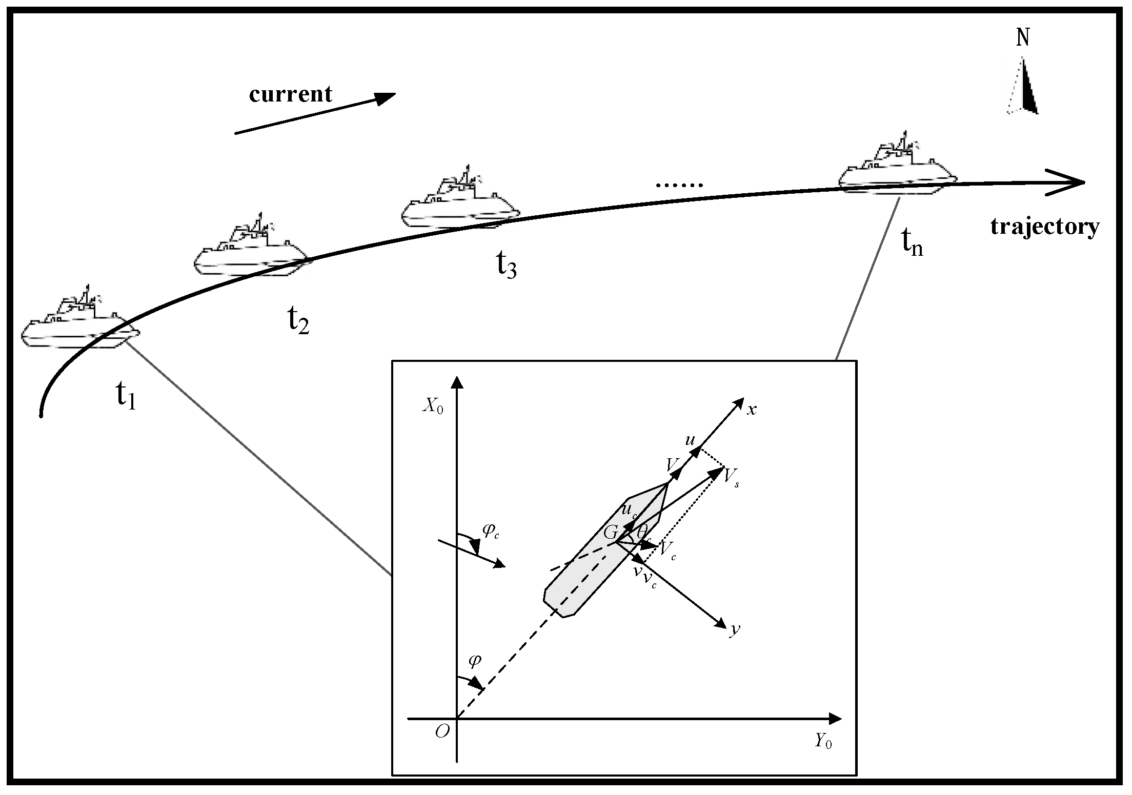
3.3. Ship Speed Correction under the Flow Field Effect

Due to the influence of water flow on the ship, the SOG values in the AIS information may be higher or lower than the actual speed value provided by the ship’s main engine, which will bring a large error to the emission calculation results. Thus, it is necessary to consider the flow field to correct the SOG values in real time.

The influence of the flow field on ship movement is shown in Figure 2. In the figure, OX₀Y₀ is the earth-fixed coordinate system, and Gxy is the ship coordinate system. V represents the actual speed provided by the main engine, Vs represents the SOG value in the AIS information, and V_c represents the current velocity predicted by simulation. u and v are the components of SOG in the ship heading and perpendicular to the ship heading, respectively. u_c and v_c are the rectangular components of V_c. θ_c is the flow angle between V and V_c.

As shown in Figure 2, the vector relationship among V_s, V, and V_c can be expressed by the following formula.

$$\stackrel{\rightharpoonup }{V_s}=\stackrel{\rightharpoonup }{V}+\stackrel{\rightharpoonup }{V_c}$$

(4)

The decomposed orthogonal of V_s can be represented by the equation group of Equation (5).

$$\{\begin{array}{c} u=V+V_c\cos {\theta }_c\\ v=V_c\sin {\theta }_c \\ V_s=\sqrt{u^2+v^{2 } } \end{array}$$

(5)

Then, the actual speed of the ship after adjustment can be obtained from Equation (6).

$$\mathrm{V}=\sqrt{V_s{}^2-V_c^{2}si{n}^2{\theta }_c}-V_{c}cos{\theta }_c$$

(6)

In this study, the flow field data output is based on an irregular triangular grid distribution, in which each grid center node contains information such as position, velocity, and flow direction. Since the flow field changes very slowly within a certain period, this paper assumes it as a constant flow to simplify the workload, which means that the physical quantities (flow velocity, flow direction, etc.) at any point in the flow field do not change with time in a day. The real-time location information of the ship can be obtained directly from the AIS data. Based on the relative position of the ship and flow field nodes, the current velocity and flow direction of the ship’s position at each moment can be determined by the principle of the nearest distance, and the SOG values from the AIS data can be modified continuously. The steps are as follows:

Step 1: The latitude and longitude coordinates in the AIS data are converted into 54 Beijing plane coordinates, which are unified with the coordinate units of the flow field.

Step 2: The distance between ship position at a certain time and each node of the flow field is calculated by iteration.

Step 3: The principle of the nearest distance is adopted to determine the flow field information of the ship position at a given time.

Step 4: Equation (6) is used to correct the SOG values to obtain the actual speed of the ship.

Step 5: By iterating Steps 2 through 4, the SOG values can be corrected in real time.

3.4. Estimation Model for Inland Ship Exhaust Emissions

3.4.1. Model Optimization

The traditional STEAM model can be represented by Equation (7), which calculates the ship exhaust emissions under different navigation conditions based on the power of the ship engine equipment multiplied by the corresponding emission factors and load factors [18].

$$E_i={\displaystyle \sum }_j{P}_j\times L{F}_j\times T_j\times E{F}_{i,j}$$

(7)

where E is engine emission in g; i is the type of exhaust emission. P represents the maximum continuous rating (%MCR) of the ship’s engine in kW; j is the type of power equipment, including the main engine and the auxiliary engine. LF is the load factor for the engines. T is the activity duration of the ship in h. EF represents the emission factor in g/kW·h.

Based on the traditional model, an optimal model considering the influence of the complex flow field in the inland river is proposed. The improved emission calculation model for inland ships is represented by Equation (8).

$$\{\begin{array}{c} E_i=P_m\times {(\frac{V}{V_{max}})}^3\times T_m\times E{F}_{i,m}+P_a\times L{F}_a\times T_a\times E{F}_{i,a}, under sailing\\ E_i=P_a\times L{F}_a\times T_a\times E{F}_{i,a}, at berthing\end{array}$$

(8)

where subscript m represents the main engine and a represents the auxiliary engine. It is worth noting that the load factor of the main engine should be a variable, which is determined by the maximum design speed and the actual speed of the ship obtained after correction under the influence of the flow field.

The emission of atmospheric pollutants from ships is closely related to the operating conditions. Taking the inland river ferry as an example, when the ship is in the navigation state, both the main engine and the auxiliary engine are working at the same time. When it is berthing, the main engine is shut down while the auxiliary engine is still running. Here, we use the sailing speed to divide the operating conditions of the ferries; that is, speed within 0–1 kn means that the ship is berthing, and a speed of greater than 1 kn means that it is sailing.

3.4.2. Model Parameters

The main parameters of the emission calculation model include the power of the main and auxiliary engine, load factor, emission factor, and maximum design speed. In general, the static information of the ship (such as engine power and maximum design speed) can be matched from Lloyd’s database or the ship registration database. In this study, the engine power and the maximum design speed of ferries were obtained through field investigation. The load factor of the main engine is calculated by Equation (1). For auxiliary engines, the Propeller principle does not apply. Since the load of the ferry auxiliary engine is relatively stable, it generally operates under the rated conditions. Therefore, following the study of Xu [31], the auxiliary load factor in this paper was set as 0.43. Many factors should be taken into account in the selection of ship emission factors, such as engine type, speed, fuel type, and sulfur content. There is a large gap in terms of the design standards, fuel quality, and energy consumption level between inland ships and seagoing ships; thus, the emission factors of ocean ships cannot be referred to directly. In recent years, there has been relevant research on the localization of the emission factors of inland river ships [32,33]. In this study, according to the relevant literature, the emission factors regarding engine/fuel type for the main and auxiliary engines of the ferry are shown in

Table 1. Emission factors of engines in g/kW·h.

Engine	Engine Type	Fuel Type	CO2	SO2	NOx	CO	PM2.5
Main engine	HSDI	Diesel oil	620	5.77	16.29	0.5	0.57
Auxiliary engine	HSDI	Light oil	690	2.12	12.0	1.1	0.29

Note: HSDI means high-speed diesel engine.

.

4. Case Study

Ferry transportation is a common water transportation mode in inland rivers, which mainly serves to connect the land transportation on both sides of the river. It constitutes an important part of the urban transportation system, especially for cities along the Yangtze River, like Wuhan and Nanjing. In this section, three ferries (which are sister ships) in the Wuhan section of the river are selected as a case study to evaluate the effect of the seasonal flow field on emission calculation. The study area is bounded in a rectangular range from 114°15′34″ E to 114°18′13″ E and 30°32′13″ N to 30°34′35″ N, as shown in Figure 3. The parameters of the three sister ships are shown in

Table 2. Basic parameters of the three sister ferries.

Parameters	Values
Length	46 m
Width	10 m
Gross tonnage	400 t
Design sailing speed	24 km/h
Main engine power	220 kW × 2
Auxiliary engine power	120 + 60 kW
Engine rated speed	1500 r/min

.

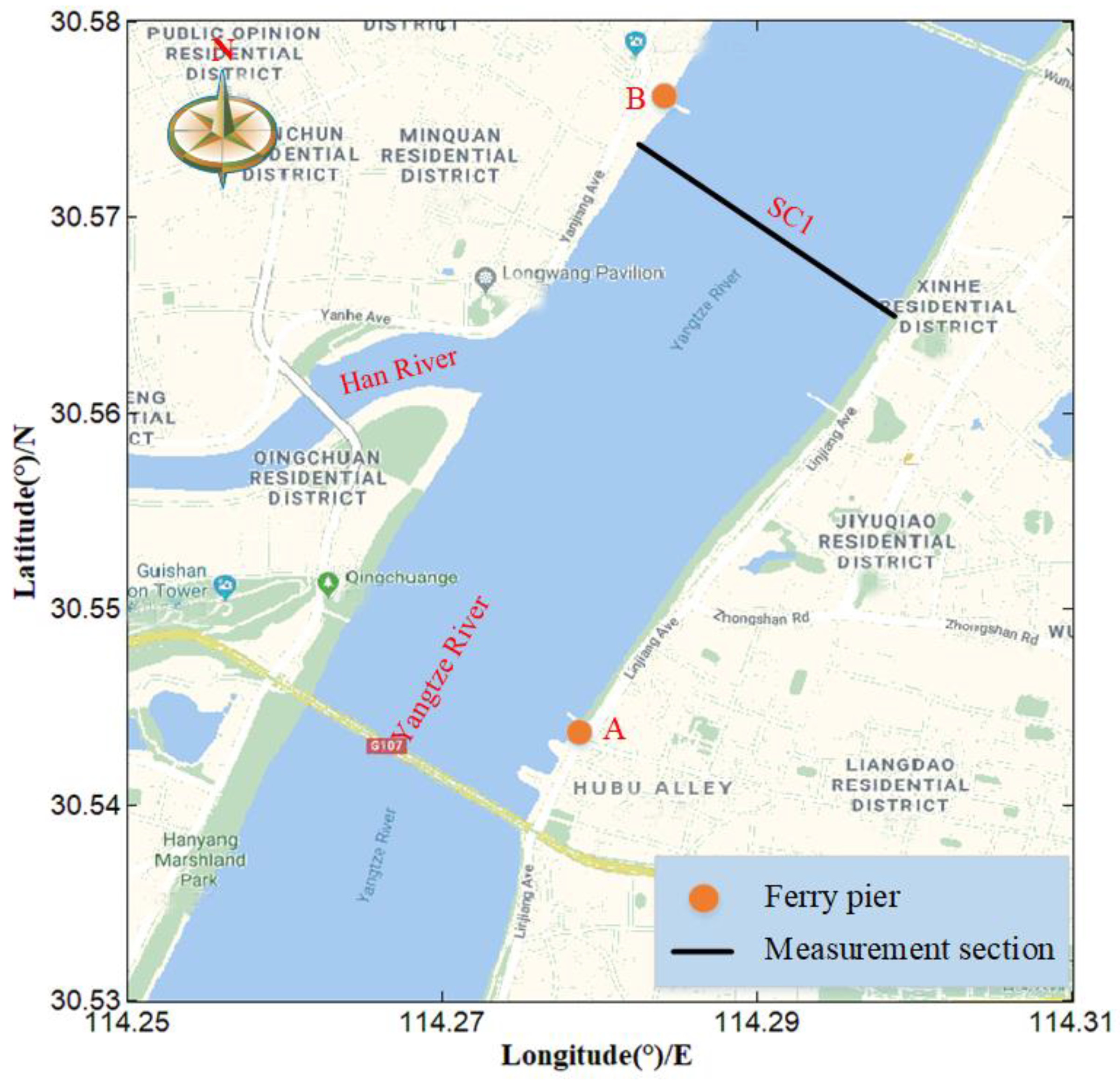
4.1. Data Acquisition

The research data are mainly divided into two categories: hydrological data and channel topographic data used for flow field numerical simulation, and ship AIS data and technical parameter data used for emission calculation.

The hydrological data were obtained from the hydrological station and the river report in the Bureau of Hydrology and Water Resources of Hubei Province (http://113.57.190.228:8001/web/Report/RiverReport), and mainly included historical water level, discharge, water depth, and other information, as well as measured velocity data. The channel topographic data came from electronic channel maps that included topographic data and boundary data, which are basic for constructing the regional flow fields.

The AIS data came from the three ferries sailing on the route from the Wuhan Customs Marina to the Zhonghua Road Marina, mainly including MMSI (maritime mobile service identity), timestamp, position information (longitude and latitude), sailing speed (SOG), heading, and so on. In addition, the technical parameters of the ferries were obtained from the local maritime bureau and other departments. They mainly include the diesel engine type, the rated power of the main and auxiliary engines, and the maximum design speed of the ship.

4.2. Numerical Simulation Experiment of the Flow Field

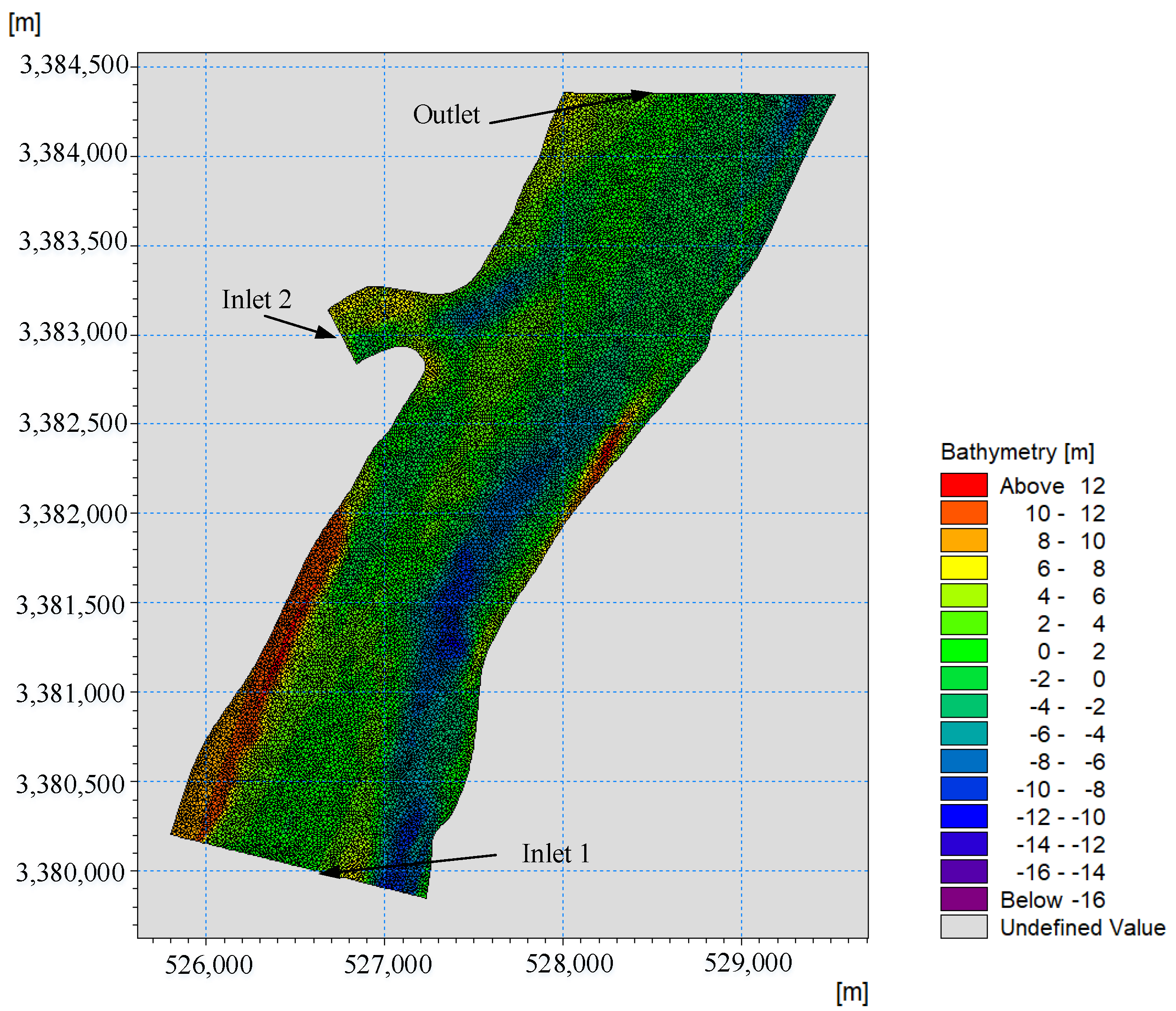
4.2.1. Terrain and Grid Generation

The calculation range of the water area was the section from the Wuhan Yangtze River Bridge to the Hankow Customs House, with a total mileage of about 4.2 km, in which the intersection of the Han River and the Yangtze River is about 0.3 km. Based on the 1954 Beijing Coordinate System and irregular triangular grid, the region is divided into 34,807 effective grids and 24,914 generated nodes. Figure 4 shows the terrain and grid map of the research area, which was obtained by interpolation according to the elevation data of the electronic channel map. The datum level is based on the 1985 National Height Datum.

4.2.2. Simulation Schemes and Parameter Settings

Considering the impact of tributary inflow on the mainstream, the flow field model in this study sets the Yangtze River as Inlet 1 and the Han River as Inlet 2 (as shown in Figure 4). Summer and winter are taken as the time background, and flow field simulation conditions are set according to the historical hydrological data of the water area in January (the dry season) and June (the flood season) of 2018, as shown in

Table 3. Simulation conditions of the hydrodynamic model.

Water Season	Initial Conditions		Boundary Conditions
	Water Level (m)	Initial Velocity (m/s)	Given Discharge of Inlet 1 (m3/s)	Given Discharge of Inlet 2 (m3/s)	Given Water Level of Outlet (m)
January	13.50	0	14,200	680	13.62
June	24.80	0	42,700	1610	24.82

.

To ensure the stability and accuracy of the flow field simulation, the time step of the model is set as 0.75 s in the dry season and 0.3 s in the flood season. The roughness coefficient is 0.02 for the main trough and 0.03 for the beach in the simulated area, and the viscosity coefficient of the flow turbulence is 1. In addition, the density is calculated in a barotropic mode, in which the salinity and temperature remain unchanged during the model calculation.

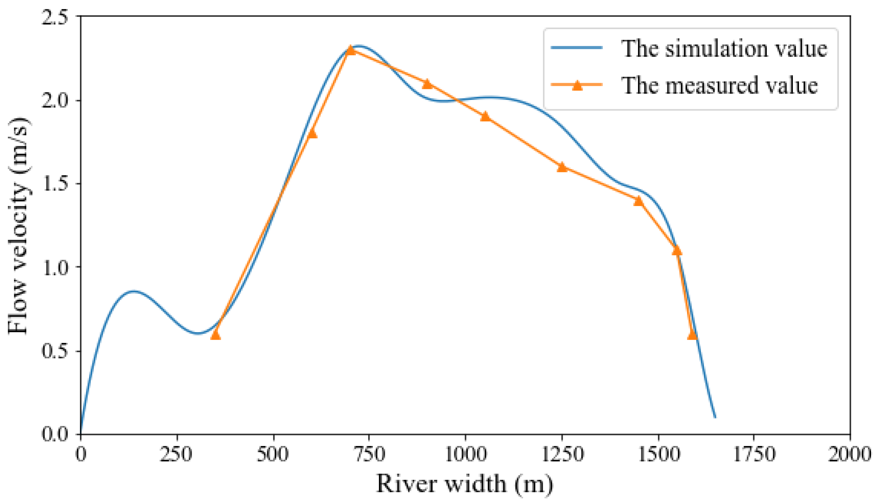
4.2.3. Model Validation

The accuracy of the numerical model of the flow field is the premise of calculation. Surface velocity data of the cross-section were measured and obtained on 22 June 2018, and were used to validate the model (Figure 3 shows the locations of the measured section). According to the data of the Hankou hydrological station, the discharge is 39,835 m³/s and the water level was 24.39 m at that time. By using the mathematical model of the flow field established in this study, the simulated velocity distribution of Section SC1 at a time under the aforementioned parameters was obtained and was compared with the measured value, as shown in Figure 5. It can be seen from the figure that the simulation results are in good agreement with the measured values, which demonstrates that the model parameter selection is reasonable, and the model has a good simulation effect for reflecting the distribution characteristics of the flow field in the study area.

5. Results and Analysis

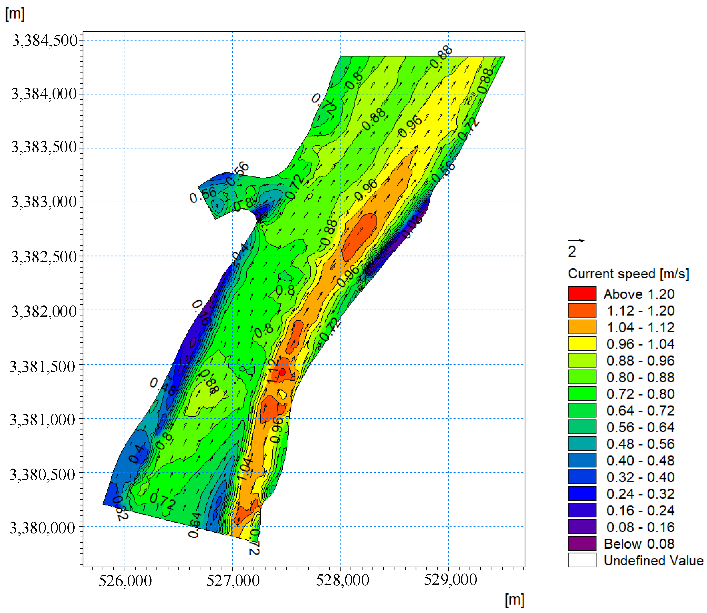
5.1. Results and Analysis of the Calculation of the Flow Field

The flow field is influenced by topography, water level, and other factors, and has different characteristics in different seasons. Figure 6 and Figure 7 show the distributions of flow field calculation results in the dry season and the flood season, respectively. In the dry season, the average velocity of the main channel is 0.80–0.90 m/s. The velocity increases with the increase of water depth, and the maximum velocity is 1.20 m/s. During the flood season, due to the increase of the water level, the average velocity reaches 1.8–2.0 m/s, and the maximum velocity at the intersection of the Yangtze River and the Han River can reach 2.8 m/s. Combined with the historical hydrological data of the area, the simulation results can accurately reflect the distribution characteristics of flow velocity and direction in different seasons.

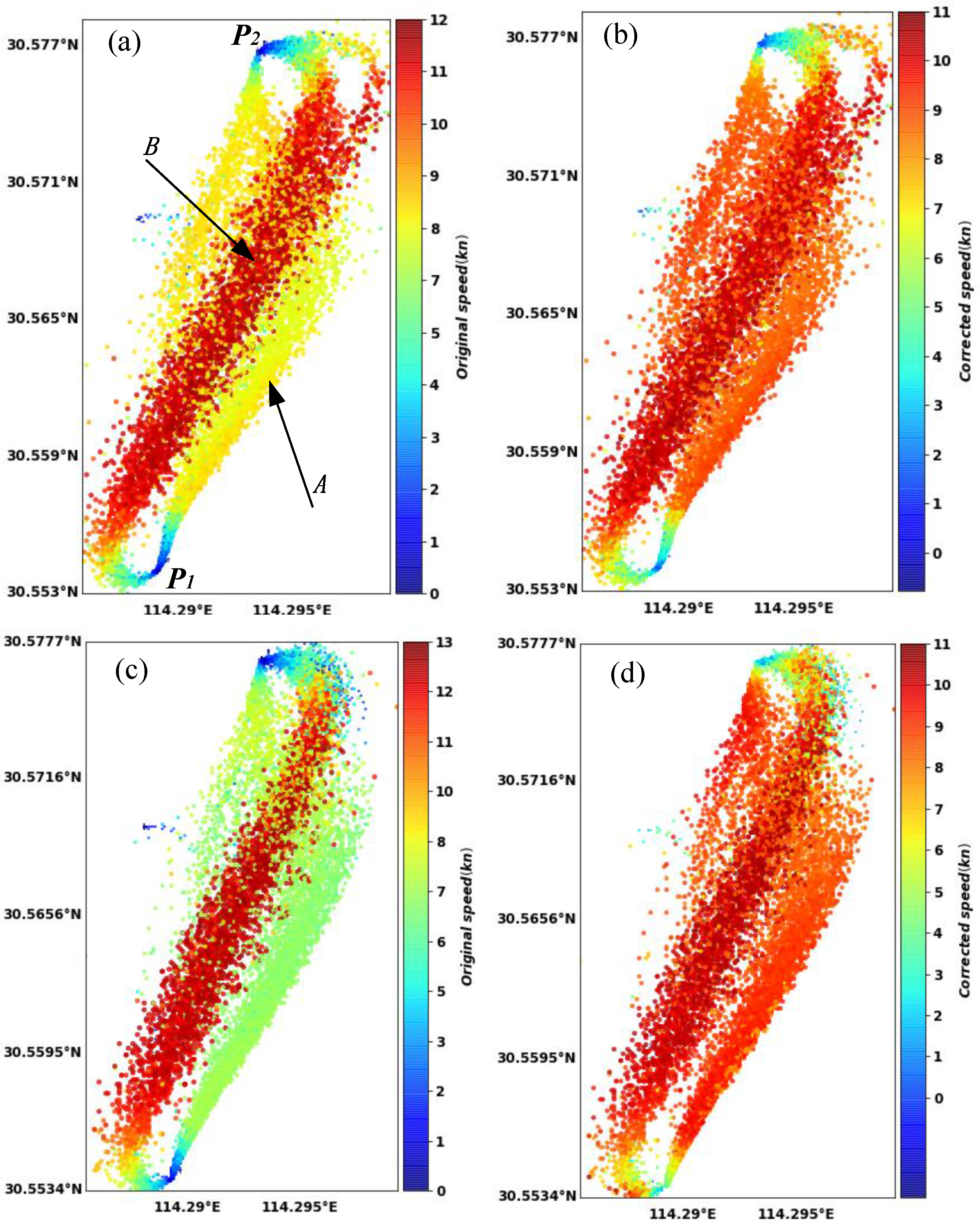
5.2. Results and Analysis of the Seasonal Flow Field Effect on Ship Speed

In the inland waters, flow velocity varies greatly at different water levels with seasonality variation; thus, the impact on the ship speed is also different. To evaluate this effect more visually, the simulated flow field data are used to correct the speed of the ferry in January and June, respectively. The spatial distribution visualization of the original speed in the AIS data and the actual speed obtained from correction was performed, as shown in Figure 8. Subplots (a) and (b) in the figure show the comparison of ship speed before and after correction in January, while subplots (c) and (d) are in June. In subplot (a), P₁ and P₂ represent the location of the Zhonghua Road Marina and Wuhan Guan Marina, respectively, while Arrow A (the yellow cluster) and Arrow B (the red cluster) represent the speed distribution of the ferry sailing up and sailing down the river.

It can be seen from Figure 8 that, due to the influence of the flow field disturbance on the ship speed, there is a relatively obvious error between the speed in the AIS information and the actual speed provided by the main engine. Especially in the flood season, the error caused by the increase of flow velocity is more obvious. We can see that when the ferry is sailing up the river, under the influence of flow resistance, the original speed in the AIS information is lower than the actual speed provided by the main engine (the average errors of these two speeds are about 1 kn in January, but 2–3 kn in June). In contrast, the original speed in the AIS information is higher than the actual speed due to the push of the current when the ferry is sailing down the river. The average errors of these two speeds are about 1 kn in January and 1–2 kn in June. Equation (1) has demonstrated that the error between the two will bring uncertainty to the emission calculation, which makes it necessary to use seasonal flow field factors in inland ship emission calculation.

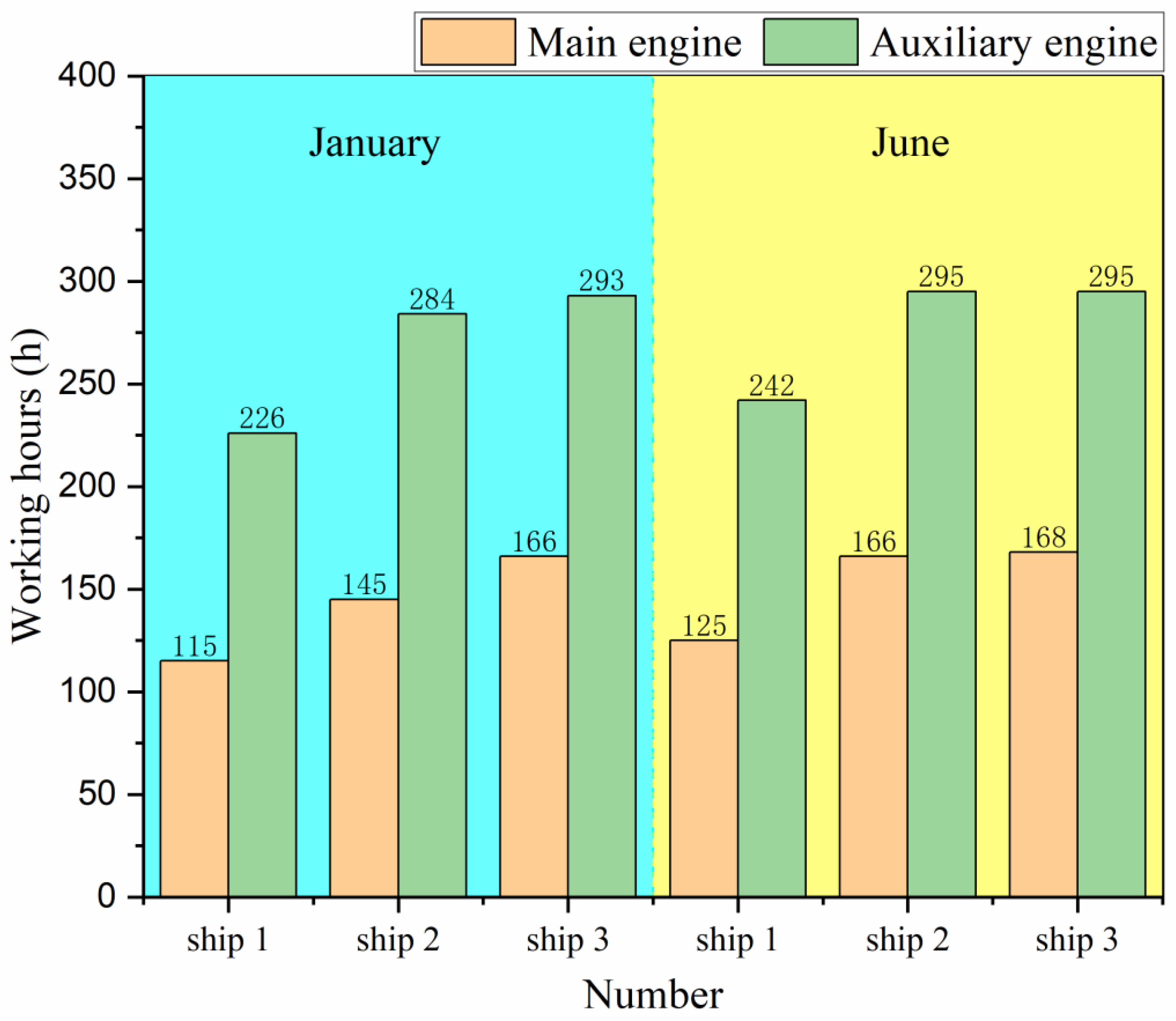
5.3. Results and Analysis of the Seasonal Flow Field Effect on Emission Calculation

To further quantify the influence of seasonal flow field on the calculation of inland ship emissions, AIS data from the three ferries were selected for exhaust emission calculation. After the data were preprocessed, there were 46,395 effective AIS records in January and 44,641 in June. Figure 9 shows the working hours of the main and auxiliary engines of the three ferries in January and June.

The traditional STEAM model and the improved emission calculation model for inland ships considering the influence of the flow field were respectively used to calculate the ship emissions. The results are shown in

Table 4. The calculation results of ferry emissions in January (unit: ton).

Number	MMSI	Group	CO2	SO2	NOx	CO	PM2.5	Total	Error
Ship 1	413932544	A	19.419	0.130	0.438	0.023	0.014	20.024	1.28%
		B	19.173	0.127	0.431	0.022	0.014	19.768
Ship 2	413932545	A	23.217	0.153	0.520	0.028	0.016	23.935	1.42%
		B	22.891	0.150	0.512	0.027	0.016	23.596
Ship 3	413932548	A	25.148	0.166	0.563	0.030	0.018	25.925	1.61%
		B	24.746	0.162	0.553	0.029	0.017	25.507

and

Table 5. The calculation results of ferry emissions in June (unit: ton).

Number	MMSI	Group	CO2	SO2	NOx	CO	PM2.5	Total	Error
Ship 1	413932544	A	21.380	0.143	0.482	0.025	0.015	22.045	13.64%
		B	18.481	0.116	0.406	0.023	0.013	19.039
Ship 2	413932545	A	30.915	0.220	0.716	0.035	0.023	31.909	13.23%
		B	26.846	0.182	0.608	0.031	0.019	27.687
Ship 3	413932548	A	23.206	0.167	0.540	0.026	0.017	23.957	21.64%
		B	18.208	0.121	0.409	0.021	0.013	18.772

, in which Group A is the calculation result when considering the influence of the flow field, and Group B is the calculation result using the traditional model.

As can be seen from Table 4, the relative errors between the total emissions of Group A and Group B from the three ferries are 1.28%, 1.42%, and 1.61%, respectively, in January. The results show that the use of the flow field model during the winter season is not necessary because the error of 1% is less than the uncertainty in the estimation of real emissions. From Table 5, the relative errors are 13.64%, 13.23%, and 21.64%, respectively, in June. The results indicate that without considering the flow field, the results of emission calculations are often underestimated, especially in summer.

In fact, ferries travelling to and from the two sides of the Yangtze River are affected by both the thrust and resistance of the current, which may offset part of the influence of the water flow on them. It is because of this offset effect that the calculation error of ship emissions is small in the dry season, while the error is still significant during the flood season. In addition, it should be noted that the flow field only affects the emission of the main engine. It can be seen from Figure 9 that the working time of the auxiliary equipment of the ferry is longer than that of the main engine. Therefore, considering the emission of the auxiliary engine will also reduce the error.

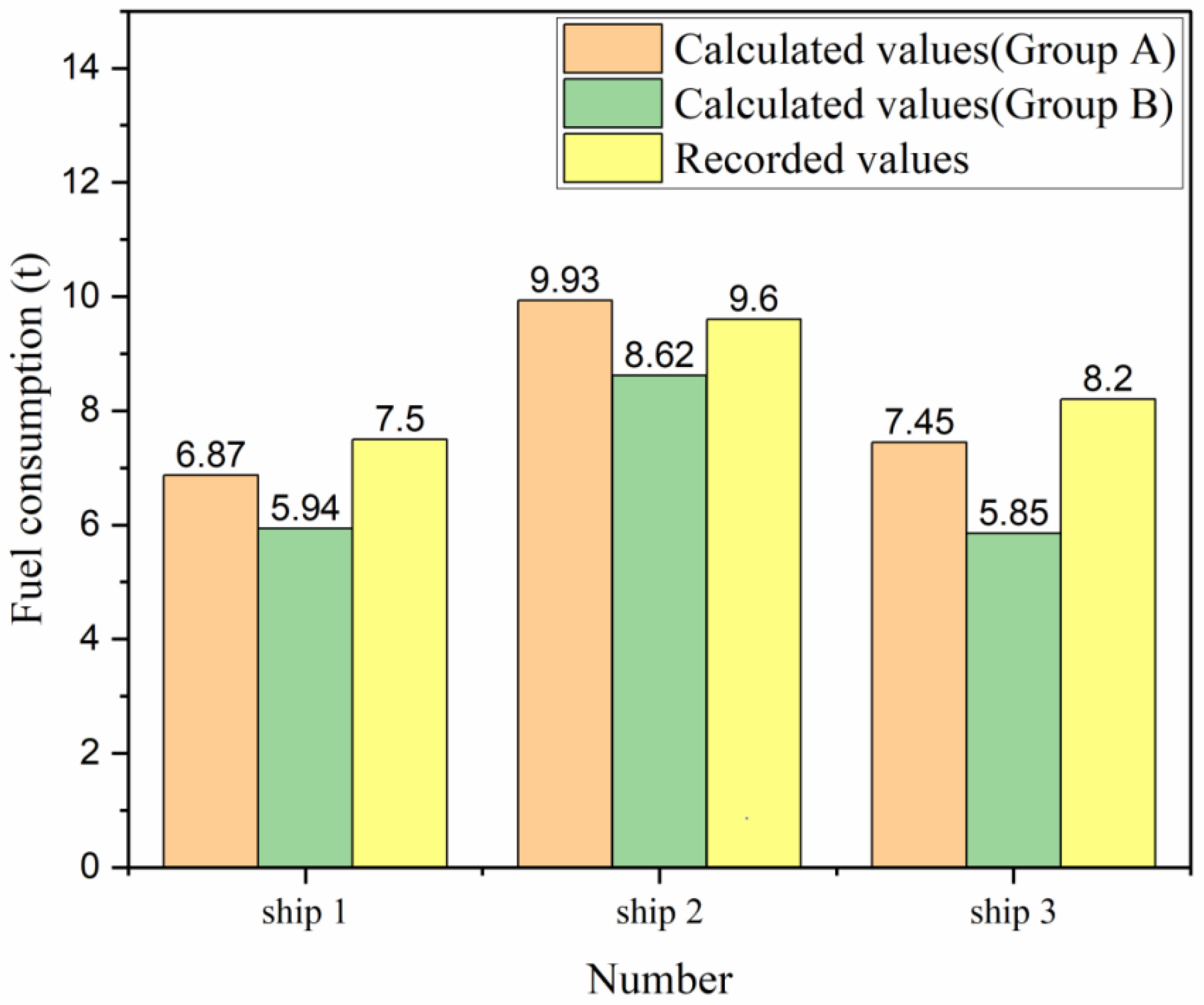
5.4. Analysis of the Effectiveness of the Improved Model

To verify the effectiveness and accuracy of the improved emission calculation model, this paper uses the backward deduction method, which means that the fuel consumption of the ferries is calculated backward by dividing the CO₂ emissions by the emission factor based on fuel consumption, and is then compared with the recorded fuel consumption. According to a research report by the International Maritime Organization (IMO) [34], the emission factor of CO₂ based on fuel consumption was selected as 3.114 t/t. The fuel consumption record report was obtained from an investigation of the ferry company; this is regarded as the real fuel consumption data.

According to the results shown in Table 4 and Table 5, the relative errors between the total emissions of Group A and Group B are 1–2% in January, while they are 13–22% in June. The use of the flow field model during the winter season is not necessary in the estimation of real emissions. To verify the effectiveness and accuracy of the proposed model, the data of CO₂ emissions from Table 5 were used to calculate the fuel consumption of each ferry in June of 2018.

In Figure 10, the calculated values and recorded values of fuel consumption of the three ships are compared. In the histogram, the orange bars represent the calculated fuel consumption of the optimized model proposed in this study, the green bars represent the calculated fuel consumption of the traditional model, and the yellow bars represent the actual values recorded in the logbook. It can be seen that the fuel consumption value calculated according to the emission results of Group A is closer to the real fuel consumption (the average error of Group A is 1.8% and that of Group B is 19.3%), which fully indicates that the proposed model is precise. That is, the proposed model can effectively reduce the error in calculation of inland ship emissions compared with the traditional model.

6. Conclusions

In this study, a calculation model of inland ship emissions considering the influence of the seasonal flow field is proposed. The main purpose was to evaluate the effect of flow field factors on ship speed and to quantify the emission calculation error caused by them. Based on the construction of the flow field model, a dynamic real-time correction method of ship speed under the effect of flow field factors is proposed to further optimize the load factor of the main engine. The proposed method can solve the error in calculating exhaust emissions of inland ships caused by water flow. Three ferries in the Wuhan section of the Yangtze River were selected as case studies to discuss the effects of different seasonal flow fields on ship speed. At the same time, to further quantify the impact of the seasonal flow field on the emission calculation, the traditional model and the improved model considering the influence of the flow field were respectively used to calculate the emissions. The results showed that the flow field in the flood season causes more errors in ship emission calculation. This indicates that without considering the influence of the flow field, the emission calculations are often lower than the actual ones, which is more significant in summer. Moreover, the calculation model proposed in this study is more accurate than the traditional model.

Emissions from inland ships have a serious impact on the atmospheric environment and the health of urban residents. In this study, an inland ferry was used as the research object for the calculation of exhaust emissions, which fills a blank in emission calculation for small ships. The proposed optimization model in this study can also be used for different types of ships, and has certain referential significance for the construction and enrichment of ship exhaust emission inventories in the Yangtze River.

However, the emission factors of the main and auxiliary engines of inland ferries were mainly obtained from relevant literature in this study, and their applicability to ferries remains to be further verified. Moreover, we just considered the influence of the seasonal flow field factors on inland ship emissions. In inland water, wind is also one of the factors that affects the movement of ships. In addition, the dead weight of the ship also influences the ship’s fuel consumption, which will affect the emissions in turn. In the future, factors such as wind and passenger capacity are expected to be added to the calculation model to make it more complete and accurate.

References

1. Zhang, Y.; Yang, X.; Brown, R.; Yang, L.; Morawska, L.; Ristovski, Z.; Fu, Q.; Huang, C. Shipping emissions and their impacts on air quality in China. Sci. Total Environ. 2017, 581, 186–198. [Google Scholar] [CrossRef] [PubMed]
2. Feng, J.; Zhang, Y.; Li, S.; Mao, J.; Patton, A.P.; Zhou, Y.; Ma, W.; Liu, C.; Kan, H.; Huang, C.; et al. The influence of spatiality on shipping emissions, air quality and potential human exposure in the Yangtze River Delta/Shanghai, China. Atmos. Chem. Phys. 2019, 19, 6167–6183. [Google Scholar] [CrossRef] [Green Version]
3. Chen, D.; Wang, X.; Li, Y.; Lang, J.; Zhou, Y.; Guo, X.; Zhao, Y. High-spatiotemporal-resolution ship emission inventory of China based on AIS data in 2014. Sci. Total Environ. 2017, 609, 776–787. [Google Scholar] [CrossRef] [PubMed]
4. Jalkanen, J.P.; Johansson, L.; Kukkonen, J. A comprehensive inventory of ship traffic exhaust emissions in the European sea areas in 2011. Atmos. Chem. Phys. 2016, 16, 71–84. [Google Scholar] [CrossRef] [Green Version]
5. Li, C.; Yuan, Z.; Ou, J.; Fan, X.; Ye, S.; Xiao, T.; Shi, Y.; Huang, Z.; Ng, S.K.; Zhong, Z.; et al. An AIS-based high-resolution ship emission inventory and its uncertainty in Pearl River Delta region, China. Sci. Total Environ. 2016, 573, 1–10. [Google Scholar] [CrossRef] [PubMed]
6. El-Taybany, A.; Moustafa, M.M.; Mansour, M.; Tawfik, A.A. Quantification of the exhaust emissions from seagoing ships in Suez Canal waterway. Alex. Eng. J. 2019, 58, 19–25. [Google Scholar] [CrossRef]
7. Chen, D.; Tian, X.; Lang, J.; Zhou, Y.; Li, Y.; Guo, X.; Wang, W.; Liu, B. The impact of ship emissions on PM2. 5 and the deposition of nitrogen and sulfur in Yangtze River Delta, China. Sci. Total Environ. 2019, 649, 1609–1619. [Google Scholar] [CrossRef]
8. Wan, Z.; Zhou, X.; Zhang, Q.; Chen, J. Do ship emission control areas in China reduce sulfur dioxide concentrations in local air? A study on causal effect using the difference-in-difference model. Mar. Pollut. Bull. 2019, 149, 110506. [Google Scholar] [CrossRef]
9. Nunes, R.A.; Alvim-Ferraz, M.C.; Martins, F.G.; Sousa, S.I. The activity-based methodology to assess ship emissions—A review. Environ. Pollut. 2017, 231, 87–103. [Google Scholar] [CrossRef]
10. Jia, P.; Wang, Q.; Lu, X.; Zhang, B.; Li, C.; Li, S.; Li, S.; Wang, Y. Simulation of the effect of an oil refining project on the water environment using the MIKE 21 model. Phys. Chem. EarthParts A/B/C 2018, 103, 91–100. [Google Scholar] [CrossRef]
11. Xu, M.J.; Yu, L.; Zhao, Y.W.; Li, M. The simulation of shallow reservoir eutrophication based on MIKE21: A case study of Douhe Reservoir in North China. Procedia Environ. Sci. 2012, 13, 1975–1988. [Google Scholar] [CrossRef] [Green Version]
12. Song, S.; Shon, Z. Current and future emission estimates of exhaust gases and particles from shipping at the largest port in Korea. Environ. Sci. Pollut. Res. 2014, 21, 6612–6622. [Google Scholar] [CrossRef]
13. Nielsen, O.K. EMEP/EEA Air Pollutant Emission Inventory Guidebook 2013: Technical Guidance to Prepare National Emission Inventories EEA Technical Report; EEA-European Environment Agency: Luxembourg, 2013; Volume 10, p. 92722. [Google Scholar]
14. Miola, A.; Ciuffo, B. Estimating air emissions from ships: Meta-analysis of modelling approaches and available data sources. Atmos. Environ. 2011, 45, 2242–2251. [Google Scholar] [CrossRef]
15. Liu, H.; Shang, Y.; Jin, X.X. Review of methods and progress on shipping emission inventory studies. Acta Sci. Circumstantiae 2018, 38, 1–11. (In Chinese) [Google Scholar] [CrossRef] [Green Version]
16. Toscano, D.; Murena, F. Atmospheric ship emissions in ports: A review. Correlation with data of ship traffic. Atmos. Environ. X 2019, 4, 100050. [Google Scholar] [CrossRef]
17. Jalkanen, J.P.; Brink, A.; Kalli, J.; Pettersson, H.; Kukkonen, J.; Stipa, T. A modelling system for the exhaust emissions of marine traffic and its application in the Baltic Sea area. Atmos. Chem. Phys. 2009, 9, 9209–9223. [Google Scholar] [CrossRef] [Green Version]
18. Jalkanen, J.P.; Johansson, L.; Kukkonen, J.; Brink, A.; Kalli, J.; Stipa, T.; Kerminen, V.M. Extension of an assessment model of ship traffic exhaust emissions for particulate matter and carbon monoxide. Atmos. Chem. Phys. 2012, 12, 2641–2659. [Google Scholar] [CrossRef] [Green Version]
19. Johansson, L.; Jalkanen, J.P.; Kukkonen, J. Global assessment of shipping emissions in 2015 on a high spatial and temporal resolution. Atmos. Environ. 2017, 167, 403–415. [Google Scholar] [CrossRef]
20. Huang, L.; Wen, Y.; Geng, X.; Zhou, C.; Xiao, C. Integrating multi-source maritime information to estimate ship exhaust emissions under wind, wave and current conditions. Transp. Res. Part D Transp. Environ. 2018, 59, 148–159. [Google Scholar] [CrossRef]
21. Zhang, Y.; Fung, J.C.; Chan, J.W.; Lau, A.K. The Significance of Incorporating Unidentified Vessels Into AIS-based Ship Emission Inventory. Atmos. Environ. 2019, 203, 102–113. [Google Scholar] [CrossRef]
22. Huang, C.; Hu, Q.; Wang, H.; Qiao, L.; Wang, H.; Zhou, M.; Zhu, S.; Ma, Y.; Lou, S.; Li, L.; et al. Emission factors of particulate and gaseous compounds from a large cargo vessel operated under real-world conditions. Environ. Pollut. 2018, 242, 667–674. [Google Scholar] [CrossRef] [PubMed]
23. Zhang, Y.; Gu, J.; Wang, W.; Peng, Y.; Wu, X.; Feng, X. Inland port vessel emissions inventory based on Ship Traffic Emission Assessment Model–Automatic Identification System. Adv. Mech. Eng. 2017, 9. [Google Scholar] [CrossRef]
24. Van, L.T.; Macharis, C. Assessing the Environmental Impact of Inland Waterway Transport Using a Lifecycle Assessment Approach: The Case of Flanders. Res. Transp. Bus. Manag. 2014, 12, 29–40. [Google Scholar]
25. Keuken, M.P.; Moerman, M.; Jonkers, J.; Hulskotte, J.; van der Gon, H.D.; Hoek, G.; Sokhi, R.S. Impact of inland shipping emissions on elemental carbon concentrations near waterways in The Netherlands. Atmos. Environ. 2014, 95, 1–9. [Google Scholar] [CrossRef]
26. Sun, X.; Yan, X.; Wu, B.; Song, X. Analysis of the operational energy efficiency for inland river ships. Transp. Res. Part D Transp. Environ. 2013, 22, 34–39. [Google Scholar] [CrossRef]
27. Wang, K.; Yan, X.; Yuan, Y.; Jiang, X.; Lin, X.; Negenborn, R.R. Dynamic optimization of ship energy efficiency considering time-varying environmental factors. Transp. Res. Part D Transp. Environ. 2018, 62, 685–698. [Google Scholar] [CrossRef]
28. Cao, Y.L.; Wang, X.; Yin, C.Q.; Xu, W.W.; Shi, W.; Qian, G.R.; Xun, Z.M. Inland vessels emission inventory and the emission characteristics of the Beijing-Hangzhou Grand Canal in Jiangsu province. Process Saf. Environ. Prot. 2018, 113, 498–506. [Google Scholar] [CrossRef]
29. Browning, L. Current Methodologies in Preparing Mobile Source Port-Related Emission Inventories; Final Report; US Environmental Protection Agency: Washington, DC, USA, 2009.
30. Danish Hydraulic Institute (DHI). MKE21: A Modeling System for Rivers and Channels Reference Manual; DHI Water & Environment: Hørsholm, Demark, 2007; pp. 1–3. [Google Scholar]
31. Xu, W.W.; Yin, C.Q.; Xu, X.J.; Zhang, W. Vessels Emission Inventory and Its Emission Characteristics on Inland River in Jiangsu Province. Environ. Sci. 2018, 40, 2595–2606. (In Chinese) [Google Scholar]
32. Xiao, X.; Li, C.; Ye, X.; Wang, R.; Yu, K.; Xie, Y.; Liao, S.; Huang, Z.; Zheng, J. Emission characteristics of gas- and particle- phase pollutants from river vessels in cruising mode. Acta Sci. Circumstantiae 2019, 39, 13–24. (In Chinese) [Google Scholar]
33. Zhang, F.; Chen, Y.; Cui, M.; Feng, Y.; Yang, X.; Chen, J.; Zhang, Y.; Gao, H.; Tian, C.; Matthias, V.; et al. Emission factors and environmental implication of organic pollutants in PM emitted from various vessels in China. Atmos. Environ. 2019, 200, 302–311. [Google Scholar] [CrossRef]
34. IMO. Third IMO GHG Study 2014; International Maritime Organization (IMO): London, UK, 2014. [Google Scholar]
Figure 1. The framework of inland ship emission estimation considering flow field factors.
Sustainability 12 07484 g001
Figure 2. Schematic diagram of the influence of flow field on ship movement.
Sustainability 12 07484 g002
Figure 3. Study area. SC1 represents the section position of measured velocity; point A is the Zhonghua Road Marina and point B is the Wuhan Customs Marina.
Sustainability 12 07484 g003
Figure 4. The terrain and grid map of the calculation simulation area.
Sustainability 12 07484 g004
Figure 5. Comparison between the simulation value and the measured value of flow velocity at Section SC1 (Q = 39,835 m3/s).
Sustainability 12 07484 g005
Figure 6. Flow field distribution in the dry season (January).
Sustainability 12 07484 g006
Figure 7. Flow field distribution in the flood season (June).
Sustainability 12 07484 g007
Figure 8. Comparison and visualization of ship speed correction. (a,c) show the original speed distribution from the AIS data; (b,d) show the corrected speed distribution after considering the influence of flow field factors.
Sustainability 12 07484 g008
Figure 9. Working hours of the main and auxiliary engines.
Sustainability 12 07484 g009
Figure 10. Comparison between calculated values and recorded values of fuel consumption.
Sustainability 12 07484 g010