Abstract
The development of adaptation indicators and metrics that can be aggregated and compared to support environmental management is a key challenge for climate experts, finance institutions, and decision-makers. To provide an operational ex-ante evaluation of alternative adaptation strategies, statistical evaluation was conducted on 1562 adaptation projects contained in the Nationally Determined Contributions (NDCs) submitted by almost all parties who signed the Paris Agreement in 2015. As a preliminary stage, we are suggesting a physical risk taxonomy derived from climate model databases and an adaptation project taxonomy using a text analysis. The second stage, consisting of an evaluation metric using a correspondence analysis between adaptation projects and risk classes, was inspired by the analogy with adaptation mechanisms in living organisms—assessing the correct correspondence between threats from the environment and adaptive solutions. It allowed us to develop a coefficient ranging from 0 to 1, expressing the degree of correspondence between adaptive measures’ categories and hazard levels, which we refer to as fitness. Our coefficient would make it possible to compare project classes with each other ex-ante or, conversely, to deduce the most relevant adaptation solutions from climate-change-related hazards. The fitness coefficient could also be used as a preliminary stage of assessment to create a short-list of adaptation projects that are relevant to address a given physical hazard with a given intensity.
1. Introduction
Adaptation to climate change has been difficult and is likely to persist as a major challenge in the future. Global warming, as well as the resulting extreme fluctuation in temperature and precipitation, creates many difficulties in various sectors, such as energy, agriculture, health, security, etc. [1,2,3,4]. Global organizations such as the Intergovernmental Panel on Climate Change (IPCC, created in 1988) and the United Nations Framework Convention on Climate Change (UNFCCC, adopted by 154 Parties in 1992 at the Earth Summit in Rio de Janeiro) were created to document climate change impacts and to develop and evaluate possible mitigation and adaptation strategies.
Mitigation should not be the only lever for action. Indeed, insufficient mitigation makes adaptation necessary. Thus, the idea that synergies between mitigation and adaptation should be promoted is now widely accepted [5,6]. In 2014, the IPCC stated that: “Adaptation and mitigation are complementary strategies to reduce and control the risks associated with climate change” [7]. In 2015, Article 7 of the Paris Agreement stated that: “The Parties shall establish the global objective on adaptation to enhance adaptive capacity, increase resilience to climate change, and reduce vulnerability to climate change (…)”. However, before this recent acknowledgement, adaptation to climate change has long remained the “poor side” in terms of thinking and funding, given the many difficulties (e.g., spatial and temporal planning) involved [8].
According to Article 4 of the Paris Agreement, countries must submit their Nationally Determined Contributions (NDCs) every five years, informing about their projects in terms of mitigation and adaptation. National Adaptation Plans (NAPs) are also available for monitoring the least developed countries, following a model established by the UNFCCC. However, in the absence of quantification of adaptation measures or an accurate assessment of adaptation projects, it is difficult for both investors and public decision-makers to assess the quality of projects and, thus, to allocate funds for their implementation. The development of expert methods leading to adaptation indicators and quantifiable parameters that can be aggregated and compared within the same adaptive issue is therefore a key challenge [9,10]. The objective of evaluating adaptation projects through the identification of similarities and the establishment of a taxonomy is to enable their comparison, selection, funding, implementation, and monitoring.
Therefore, we pursue two objectives using an analysis of more than 1550 adaptation projects contained in the NDCs submitted at the 21st Conference of Parties (COP-21) at the end of 2015 in Paris. First, we establish a risk taxonomy using the literature and an adaptation project taxonomy using an automatic text analysis. By developing classes of adaptation projects, we aim to distinguish between adaptation measures, taking into account identified physical risks (storms, floods, droughts, heat waves)—without, however, treating each situation specifically—to allow comparability. Second, we propose an evaluation metric using a correspondence analysis between classes of risks and classes of projects.
2. Literature Review
Adaptation is a polysemic concept. For example, Smit and Skinner [11] define it as “one of the policy options in response to climate change impacts”, while Adger et al. [12] use a 2001 IPCC definition, stating that adaptation is “an adjustment in ecological, social, or economic systems in response to observed or expected changes in climatic stimuli and their effects and impacts in order to alleviate adverse impacts of change or take advantage of new opportunities”. In 2007, the IPCC defined adaptation as “adjustment in natural or human systems in response to actual or expected climatic stimuli or their effects, which moderates harm or exploits beneficial opportunities” [13], and used a very similar definition in 2014: “Adaptation is the process of adjustment to actual or expected climate and its effects in order to either lessen or avoid harm or exploit beneficial opportunities” [7]. These IPCC definitions refer to two concepts that have been distinguished in the literature [14]—on the one hand, adaptation means taking measures to reduce impacts of harmful events and to adapt progressively to variable risks and stimuli (gradual rise in sea level, increase in temperature). On the other hand, the coping capacity refers to short-term reactive efforts implemented rapidly to counter the immediate impacts of catastrophic change (such as droughts, floods, or epidemics) [15,16]. Both concepts also apply to the broader definition of resilience, i.e., the capacity of a system to anticipate, learn, adapt, and recover from a disastrous event [17]. Resilience has become a key concept of international politics consisting of Disaster Risk Reduction [18]. Several authors stressed the complex relationship between an ex-ante vulnerability and an ex-post resilience [19]. Vulnerability drivers do not systematically predict resilience, as the latter concept is not only determined by pre-existing conditions to the crisis (risk), but also by the post-catastrophe situation [20]. In this article, we do not distinguish these two concepts of coping and adapting, as we only consider the correspondence between a class of risk and the kind of adaptation answer that was envisaged. Our approach could reduce risks by providing an ex-ante assessment of the relevance of adaptation choices. Resilience provides a larger framework to deal with vulnerabilities preventively and ex post—in the short term and long term—for decision-makers and project leaders to strengthen and adjust the necessary adaptive measures once they have been chosen.
Decision-makers, project leaders, and funders agree on the usefulness of creating classes or categories for both climate vulnerabilities and adaptation measures, as described below. A taxonomy on which everyone would agree would allow, among other uses, the prioritization of actions in relation to the issues at stake and, above all, the comparison of projects’ relevance, efficacy, or efficiency with each other.
In 2014, the IPCC [7] released a comprehensive report on future climate changes, risks, and impacts, as well as on possible pathways for adaptation and mitigation. More recently, Mora et al. [21] studied the risks related to climate change as an expression of hazards and their frequency by highlighting already existing risks and their possible amplification in the future. As the necessity for adaptation actions is clearer, the foundations of a framework for assessing the relevance and the monitoring and evaluation (M&E) of adaptation projects have been laid [22]. The IDDRI (the French Institute for Sustainable Development and International Relations) proposed an approach that consists of assessing progress on adaptation directly at the global level so as to avoid being locked into the political and diplomatic barriers inherent to any country-level reporting system. Training tools and modules for Parties to the UNFCCC have been proposed, such as those of the Consultative Group of Experts [23], and others from international bodies such as the EU Climate support tool, the UK Climate Wizard, the US Agency for International Development (USAID) framework, and Climate Risk Informed Decision Analysis (CRIDA). These are adaptive project planning methods, based partly on vulnerability and needs assessments, which belong to the broader category of “adaptive management”. Adaptive management considers decisions as an iterative process [24], and “uses management actions as experiments to provide data supporting, or failing to support, competing hypotheses when there is uncertainty regarding the response of ecological systems to management activities, to better meet management objectives over time” [25]. However, adaptive management is applied as the project is developing, and uses a deductive method to increase the resilience of the system [26], but not to predict the best solution ex-ante. In this article, we are working exclusively ex-ante, and we use the deductive approach based on the NDCs and their successive revisions in order to describe classes of adaptation projects.
Bosello et al. established several criteria for classifying adaptation projects based on an early work from Smit et al.: purposefulness (autonomous to planned), timing (anticipatory to reactive), temporal scope (short term to long term), spatial scope (localized to widespread), function (protect, retreat, accommodate, or prevent), form (structural, legal, or institutional), and valuation of performance (effectiveness, efficiency, equity, feasibility) [27]. More recently, Biagini et al. [28] classified 92 adaptation projects into 10 categories according to their own framework. This taxonomy was then applied to the coastal sector, for example [29]. Other sectors have been analyzed according to Smit et al.’s framework, such as agriculture or transport [11,30]. In addition, an attempt has been made to classify projects according to four modes of governance [31]. It appears, however, that most of the analyses involve specific sectors or places without real prospects of more global applications. Our aim is to statistically identify constants and common features among climate situations and adaptation actions observed at the global level and recorded in countries’ NDCs.
In addition to being designed at very local levels, adaptation projects address a wide variety of sectors and ecosystem sub-levels. They are also projects with uncertain results, as they are developed over long time frames during which the social and scientific contexts evolve [12,22,32]. The choice of an adaptation option depends on and influences the vulnerability of the environment to which it applies, i.e., “the degree to which a system is susceptible to, and unable to cope with, adverse effects of climate change, including climate variability and extremes” [13]. Recent scientific literature has attempted to define a taxonomy of vulnerabilities [15]; however, such a taxonomy also presents difficulties, as perceptions of vulnerability also vary according to the socio-economic context [33]. Although it is difficult to establish a universal classification of adaptation projects and to find relevant indicators [34,35], a more comprehensive approach to evaluating adaptation projects is recommended [9,36]. According to Berrang-Ford [37], an intergovernmental comparison is possible through transferable and scalable concepts that are evaluated by governments themselves. Similarly, the report of the French Economic Council for Sustainable Development [8] shows that for specific projects, it is possible to find similarities that allow a comparison. For the sake of an overall synthesis, indicators must be able to be aggregated and, therefore, have common points [38,39].
3. Materials and Methods
The evaluation of NDCs’ adaptation projects has so far been carried out mainly from the point of view of the technical or financial support needed to implement the announced measures [40,41]. Here, we are building a new metric to assess a project category’s relevance depending on the risk it is addressing. We therefore grouped the adaptation projects of the NDCs into risk categories and then adaptation project categories, and conducted a correspondence analysis to quantify the vectoral distance (fitness) of a project category to the targeted level of vulnerability in a specific category of risk. The process of work is displayed in Figure 1. The intention to simplify in our analysis, was to be non-systemic, voluntarily ignoring the possible interactions between stakes and between adaptation actions at this stage of the study, as physical hazards and intensities were only characterized at the national level due to the lack of regional data for the whole world. In addition, the precise geographic area where the project is meant to be implemented is rarely mentioned in NDCs or NAPs, making it difficult to conduct analysis at the regional level. This modeling of a few variables explaining the issues and choices is intended to describe reality to obtain a quick but nevertheless significant result.
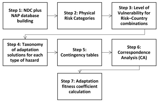
Figure 1.
Diagram displaying the working process. The methodology for each step is detailed below.
The intuition tested in this contribution came from an analogy using the adaptive biological mechanisms observed in the living: “The ‘adaptations’ of an animal, its anatomical details, instincts, and internal biochemistry, are a series of keys that exquisitely fit the locks that constituted its ancestral environments” (Richard Dawkins, www.edge.com). Our project is thus to quantify some correspondence, affinity, distance, or relevance between a class of adaptive solutions (“keys”) and a class of vulnerabilities related to climate change (“locks”).
3.1. Step 1: NDC Plus NAP Database Building
Our database of projects focused on climate change adaptation uses two main sources. The first includes 1562 adaptation projects contained in the NDCs submitted to the Paris Accord in 2015. The second includes 547 High-Priority Projects (HPPs) from the National Adaptation Plans (NAPs) provided since 2011 to the UNFCCC by the fifty least-developed countries, which need adaptation the most [42,43,44]. When a project consigned in the NDC of one of the least-developed countries was not explicit enough, we used the NAP description of the same project.
The database is thus composed of 1562 lines, each presenting an adaptation project and its country of adoption.
3.2. Step 2: Physical Risk Categories
Adaptation cannot be detached from the climate-change-induced hazard’s impacts that it claims to reduce, which is why authors have focused a great deal of attention on articulating vulnerability assessment in relation to the challenges posed locally by climate change [45,46]. However, while vulnerability is defined for a specific system, sector, or region (as a degree of sensitivity to a risk), physical risk applies to all system, sectors, and regions. Therefore, we chose to associate the projects in the NDCs with physical risks, which are external threats.
We drew up a list of eight physical risks that adaptation projects were designed to mitigate, drawn from Mirza [15], with addition of the “Unknown hazard” category, since many projects are not necessarily focused on specific threat types:
- Drought
- Flood
- Heat waves
- Sea level rise
- Storm
- Rainfall
- Temperature increase
- Unknown hazard.
Each of the 1562 adaptation projects was reviewed by the authors, and assignment to a category was made; the categories of risk are specified in our database for each project. The same project can be associated with several risk categories for future analyses.
3.3. Step 3: Level of Vulnerability for Risk–Country Combinations
We associated a level of vulnerability with each country–risk pair for each of the projects using the Climate Vulnerability Monitor developed by the DARA organization and the Climate Vulnerable Forum. DARA is a non-profit organization aiming at improving humanitarian aid performance by conducting evaluations, research, and policy studies. We chose to work with DARA’s Vulnerability Monitor instead of the vulnerabilities sometimes described within NDC documents in order to preserve the independence from national or supranational interests, and because the vulnerabilities were better documented. Our calculations can be run again using other databases, or when DARA issues an updated version of countries’ vulnerabilities. No vulnerability is assigned to “Unknown hazard” and “Precipitation” in this repertory, as information was not available. We therefore did not calculate the coefficients for these categories. Because the adaptation projects are designed to be implemented at national scales and the precise locations of the implementations of these projects are rarely given in the NDCs, our reference vulnerability is that of the national level, despite potential significant variations within countries.
The estimates of the levels of vulnerability (in the sense of the hazard, excluding social and economic issues) are available in the selected bases for 2010 and 2030. We have chosen to work with 2010 data, with the assumption that a country tends to base its measures on its “current” situation (i.e., the situation in 2011 for NAPs and 2015 for NDCs), given that the stakes related to adaptation actions are often already a reality. Thus, each project is no longer associated with a risk, but with one of the following four levels of vulnerability to this risk: LowModerate, High, Severe, and Acute, which allows their quantitative comparison.
3.4. Step 4: Taxonomy of Adaptive Solutions for Each Type of Vulnerability
A code for an automated text analysis was developed in R by the authors and was used as part of a three-step method analysis. The code is available as supplementary material.
First, the code analyzed the frequency of words describing the projects associated with a certain type of risk that were gathered in our database, the classification of these occurrences, and links from the most important to the weakest, which allowed the creation of project categories.
Then, the analyzed projects were manually distributed in the created categories. One project can correspond to several categories; in this case, they were each attributed to one of these classes. The text analysis process was restarted in a more detailed way on the projects not assigned at this stage, and this step was repeated until all the projects were classified (or only a few remained to be assigned manually).
The number of categories created for each risk is given in Table 1. The names of the categories and the number of projects per category are available in the results section and in Appendix A.

Table 1.
Number of project categories created for each risk class.
Finally, an expert (and manual) interpretation of the stakes of each risk class and each adaptation solution class led to the construction of a tree structure.
3.5. Step 5: Contingency Tables
For each type of risk, we constructed contingency tables with the classes of adaptation projects determined in the previous step in columns, and the four levels of vulnerability in rows.
Our ambition is to use as much information as possible from the contingency tables. The variables’ distribution across columns is one important feature to utilize. That is the reason for why we chose to carry out a correspondence analysis (CA). Indeed, a CA makes it possible to study the statistical correspondence between several qualitative variables as well as the dynamics between different variables that could not be identified solely based on the contingency table. A CA also allows the study of the possible relationship between the items considered in the rows (adaptation project categories) and the items considered in the columns (hazard intensities).
3.6. Step 6: Correspondence Analysis (CA)
This statistical method has been used occasionally in the literature to guide the choice of adaptation decision-makers. For example, Hajer et al. [47] use the multiple correspondence method in the livestock sector with respect to their relative adaptation strategies for increasing water capacity for livestock and crop production and improving livestock and housing conditions. However, such analyses are rare due to the singular, local, and, at first glance, incomparable nature of the impacts, vulnerabilities, and adaptive responses.
Here, we applied the CA method to each of our contingency tables (one for each hazard). The CA allowed us to define a new vectoral space, composed of as many dimensions as there are variables (hazard vulnerabilities) in the contingency table. These dimensions were constructed from the values contained in the contingency table. Thus, each project category contributed to a certain degree to the construction of each dimension.
Our correspondence analysis is the result of two principal component analyses (PCAs). One PCA was carried out on the rows (adaptation project categories) and another PCA on the columns (vulnerability levels). The PCA allows a large part of the sample’s variance to be expressed in a reduced number of dimensions, thus facilitating the graphical representation of the data. Indeed, as each dimension in the newly formed vectoral space contains a part of the variance (i.e., information) of the original contingency table, one can obtain a simplified vision of reality while preserving a certain level of information (by keeping a large percentage of the variance explained). In our analysis, we kept the first three dimensions (instead of the initial four levels of vulnerability), which define at least 80% of the variance for the different vulnerabilities. For each dimension, the variables (levels of vulnerability) and individuals (project classes) have coordinates, allowing us to position each of them in the vectoral space.
3.7. Step 7: Adaptation Fitness Coefficient Calculation
The method consisted of calculating the vectoral distance obtained via the CA between all categories of projects and all levels of vulnerability within a single risk class, and then constructing a score between 0 and 1 using the minimum and maximum distances observed in the entire sample to normalize the distances. As each hazard intensity and each project class have coordinates in the three-dimensional vectoral space, we can compute a distance between each project class and each hazard intensity. The vectoral distance between an environmental key and hazard intensity is calculated as follows:
where is the coordinate of environmental key i for the first dimension, and is the coordinate of hazard intensity j for the first dimension.
At this point, we have vectoral distances that are expressed numerically. The smaller the distance, the greater the link between project class and hazard intensity.
Vectoral distances are then normalized between zero and one, with the following transformation:
where is the vectoral distance between environmental key i and hazard intensity j. The maximum () and minimum () vectoral distances are taken for one hazard, with the four intensity features characterizing it.
Hence, we can define the fitness coefficient, expressed between zero and one, with the following transformation:
The closer the coefficient is to the value of “one”, the smaller the vectoral distance between the project class and the vulnerability level is, and, thus, the more the adaptive action is statistically “attracted” to this vulnerability level. By “statistical attraction” between classes of projects and vulnerability levels, we mean that these classes share similarities in their construction, as their coordinates in the different dimensions are close. As those choices are supposed to be rational and because we are comparing all projects described in the NDC documents, we assume that the smaller the distance between adaptation project class and hazard intensity, the higher the relevance of an adaptation project choice.
This calculation was made for each hazard in the taxonomy. The value obtained for the fitness coefficient is obviously dependent on the width of the categories. These classes have been constructed wide enough to group together a satisfactory number of solutions to be compared, without, however, losing the unambiguous meaning of the class.
4. Results
As a significant example, below, we only present the results of the analysis of projects assigned to the “Flood” risk. Similar analyses were conducted for the other seven risk categories and are presented in Appendix A.
The text analysis of adaptation projects assigned to the “Flood” class allowed us to construct a taxonomy in 27 categories, as shown in Figure 2.
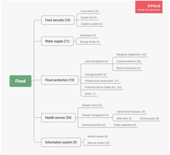
Figure 2.
Taxonomy of adaptation projects associated with the “Flood” class. The number of projects associated with each category is specified in brackets.
The projects in each class were then assigned to the level of vulnerability to flooding in their country of adoption, resulting in the construction of a contingency table (see Table 2).
Table 2.
Contingency table for the “Flood” class.
Table 2 already provides us with information on the distribution of project types. For example, 52% of “Warning system” measures are taken for a LowModerate vulnerability level. A total of 31 of the “Health service” measures are taken for a LowModerate vulnerability level, which represents more than 30% for the entire meta-category.
We then conducted a statistical analysis to obtain a quantification of the relevance of a class of projects to address a given level of vulnerability. A CA carried out on this table allowed us to calculate the fitness coefficients of the different project categories (see Table 3 and Table 4).
Table 3.
Adaptation fitness coefficient (between 0 and 1) calculated for adaptive project sub-categories associated with “Flood” risk.
Table 4.
Adaptation fitness coefficient (between 0 and 1) calculated for adaptive project meta-categories associated with “Flood” risk.
Sub- and meta-categories were analyzed separately. The calculation of fitness coefficients considering all twenty-seven categories was also carried out (see Appendix A). For this risk class, the sub-category “Land management” was analyzed together with the meta-categories as well, since this is an important category, which here includes sixty-eight projects.
Here, we can see that the “Health service” measures have a high fitness for a LowModerate vulnerability level, which is consistent with what we noted earlier in the contingency table. However, this new analysis tells us that these measures are even more relevant for a High vulnerability level, with a fitness of 1. In addition, the meta-categories “Water supply” and “Flood protection” appear to be relevant (fitness of 0.94 and 0.90, respectively) with respect to an Acute vulnerability, which was not obvious at first glance on the contingency table. This result can be refined by the sub-category analysis: In the “Water supply” category, it is the “Watershed” class that presents the highest score for an Acute vulnerability.
5. Discussion
Each step of the method is debatable. In this section, we detail the limitations of our approach and justify our decisions. We also discuss the future of the fitness coefficient and how it can be improved.
5.1. The Taxonomic Approach
The database of adaptation projects was built from two heterogeneous sources; the number of projects differs and the HPPs are much more detailed. This led us to look for more information in the NAPs when the NDCs were too succinct, and may lead, overall, to an overweighting of the least-developed countries. However, without ruling out any risk of bias, countries that have adopted NAPs have been able to benefit from a financial fund for least-developed countries set up by the Conference of the Parties (COP). It can therefore be assumed that differences in resources did not significantly affect the choices of countries that submitted their NAPs compared to those that submitted only their NDCs.
Regarding the universality of the database, a review of the consultation and bidding process undertaken in 2014 and 2015 by multilateral development banks for the benefit of the Parties to the UNFCCC led us to formulate the hypothesis that the adaptation measures recorded in the NDCs were very often designed by independent experts, recommending specific actions for each country, and were designed in a rational manner with regard to climate issues and available knowledge (climate models, knowledge of ecosystems, etc.), even if they were sometimes merely sketching well-documented climate planning. Thus, for the sake of the argument, we considered this 2015 database from the UNFCCC repertory representative of an independent position of each country. When this was not the case (application of routines or mimicry between several countries, interventions of the same consultants, crude cross-cutting recipes, etc.), national choices should become more specific and independent each time as the successive revisions of national adaptation documents are submitted (with two major stages in 2020 and 2025). We acknowledge the biases that may arise from potential common decision-makers across countries and the lack of a “bottom-up” type of process in the development of most of these NDCs without this contradicting our hypothesis of independence as a first approximation.
The risk allocation stage (step 2) is questionable on several points—the categories selected (it would have been possible to add others), but also the subjectivity of the association, which makes errors and inconsistencies possible. In fact, the association is not based on any previously documented method. Moreover, some projects addressing multiple risks have been attributed to a specific risk if it is dominant. The ranking, in general, does not capture the effects of projects on different risks at the same time.
In the third step of the method, we used a characterization of vulnerability levels at the national level to allow an initial analysis. Vulnerability assessment at a national scale is not new in the literature. Studies have shown that it is possible to construct an exposure score for a given climate risk [48]. We used the Climate Vulnerability Monitor developed by DARA and the Climate Vulnerability Forum because they appeared to be independent of national or supranational interests and well-informed. However, other baseline choices would have been possible. Regional climate downscaling could also be more accurate.
Finally, the project taxonomy was constructed depending on the prior step of risk assignment. However, we believe that the possible mistakes are too few in relation to the sample size to have an impact on the result of the statistical analysis. Nevertheless, the assignment of projects to a category was also subjective and depended on the correct interpretation of the descriptive terms of the categories. Since one project can belong to several categories, it will be accounted for several times in the contingency table. We do not believe it is a problem, however, as it allows for broader projects to have more weight. Moreover, such a taxonomy does not allow for the precision of the projects to be taken into account: A very detailed project may find itself isolated if it is alone in a category, or, on the contrary, drowned among fuzzier projects if it is attributed to a broader category. This justifies the importance of taxonomic construction into meta-categories and sub-categories.
5.2. The Adaptation Fitness Coefficient
Based on a statistical analysis, the value of this coefficient depends on the initial sample and the number of projects related to a level of vulnerability: The fewer the projects, the more the score will be influenced by a small variation in the sample. In addition, CA is a method that is very interested in the sample variation; distribution across intensities is very important in the construction of the new vectoral space. Hence, a rather even distribution, such as that for “Warning system” below (see Table 5), will display lower fitness coefficients than a more concentrated distribution (such as for “Monitor system”), even if the number of occurrences is lower. Six times out of eight, a “Monitor system” was chosen for a LowModerate vulnerability to “Flood”. On the other hand, “Warning system” was chosen 13 times out 28 for LowModerate situations. “Monitor system” scored a higher fitness than “Warning system” for LowModerate vulnerability to “Flood”, even though the number of occurrences is lower for this pair.
Here, a project category will have a high fitness for a given level of vulnerability if several countries have used an adaptation project of this category to provide an answer to this specific level of vulnerability.
In addition, the significance of the fitness score depends on our hypothesis about independence discussed in the preceding section.
Finally, it is important to mention that the coefficient is normalized between 0 and 1; however, this normalization is done within the whole risk class, and not for only one level of vulnerability, allowing us to compare solutions between intensities. For weighting purposes, it was also possible to construct a score in relation to the variation from the mean, which would have made it possible to put the many extreme scores we obtained into perspective.
5.3. Prospects and Further Work
The overall approach of the study is not challenged by the limitations discussed above. Indeed, changes to the margin remain possible for the attribution of risks (or the attribution of projects to a category) during a reviewing process. Ideally, countries should more clearly indicate the risks that their projects claim to address in their NAPs or NDCs.
The progressive increase in the number of adaptation projects and their improvement—notably, by raising the objectives, strengthening national climate teams, and improving regional climate models in predictive analysis, all within a new transparent framework—should make it possible to consider a renewed statistical treatment of the model developed here based on the successive revisions of the NDCs planned in the Paris Agreement. Article 4 of this Agreement calls for these documents to be updated every five years, starting with a new submission of updated targets and means in 2020–2021. The new NDC database “version II” could be screened using our statistical method. It would allow us, on the one hand, to validate the taxonomies: As the transparency increases and the choices of solutions to address a specific risk converge, the taxonomy should be more precise and robust to changes. On the other hand, it would help validate the values of the fitness coefficients. A similar exercise could be carried out in 2025, with new NDCs displaying raised targets in the context of increased transparency. As the objectives and transparency of adaptation actions are progressively updated and strengthened, the NDCs in their successive versions would constitute an example of mankind’s reference system for adaptation choices, often in relation to cross-cutting issues. The comparison of one version with another of the NDCs and NAPs, as well as between stakes, intensities of vulnerabilities, and fitness values for each level of vulnerability, will be rich in lessons.
We are aware that a characterization of vulnerabilities at a finer level (regional, for example) would allow a more precise analysis of the correspondence between “keys” (solutions) and “locks” (risks). A complementary analysis using hazard projections from regional climate models could be undertaken on this same 2015 database and, thus, constitute a more accurate version of a reference frame of climate solutions and challenges.
It would also be relevant to renew the statistical analysis according to risks projected for 2030 or 2050 in order to complete this analysis of national risks in 2010. This year, which belongs to the past, is, of course, better described than a projection, but does not contain all the elements for assessing adaptation choices.
6. Conclusions
A statistical analysis of 1562 adaptation projects recorded in the NDCs submitted by Parties to the UNFCCC in 2015, cross-referenced with national climate hazards, enabled us to develop a fitness coefficient. Its values, evolving between 0 and 1, indicate the mathematical correspondence between adaptation solutions and climate challenges. We believe that this new metric provides useful ex-ante evaluation of the relevance of national adaptation choices given the issues at stake within the reference framework that was set for humanity’s choices. The usefulness of the fitness coefficient relates to the evolution of this fitness value thanks to successive versions of the NDCs and the evolution of climate hazard projections over time. This new metric also allows international comparisons for classes of solutions and classes of risks. To enable these comparisons between projects and between vulnerabilities, we propose a taxonomy of risks and adaptation choices with a universal vocation. Our medium-term ambition is to be able to refine those statistical estimates by using improved regional climate models and by screening more transparent and more documented adaptation projects through successive versions of NDCs and NAPs. Such ex-ante metrics will provide finance institutions with additional information on the projects submitted for funding in a comparative manner, allowing them to keep only the most relevant ones for further consideration.
Author Contributions
Conceptualization, J.B. and E.F.; methodology, E.F., C.L., and J.B.; software, C.L. and E.F.; validation, J.B. and E.F.; formal analysis, E.F.; investigation, J.B. and E.F.; resources, J.B., E.F., C.L., and B.B.; data curation, J.B., E.F., C.L., and B.B.; writing—original draft preparation, J.B., E.F., C.L., and B.B.; writing—review and editing, J.B., E.F., and B.B.; supervision, J.B. and E.F.; project administration, J.B., E.F., and B.B. All authors have read and agreed to the published version of the manuscript.
Funding
This research received no external funding.
Acknowledgments
Translation: Tuddenham, Mark (Citepa); consulting and pre-reviewing: Linkov, Igor (US Army Corps of Engineers, Concord, Massachusetts, USA) and Galaitsi, Stephanie (Stockholm Environment Institute, US Center, Somerville, USA).
Conflicts of Interest
The authors declare no conflict of interest.
Appendix A
Appendix A.1. Flood
Table A1.
Adaptive Fitness Coefficient (between 0 and 1) calculated for adaptive project categories associated with “Flood” risk.
Table A1.
Adaptive Fitness Coefficient (between 0 and 1) calculated for adaptive project categories associated with “Flood” risk.
| Fitness All Keys | LowMod | High | Severe | Acute |
|---|---|---|---|---|
| Coastal protection | 0.89 | 0.87 | 0.53 | 0.53 |
| Crop variety | 0.80 | 0.58 | 0.52 | 0.88 |
| Disease control | 0.55 | 0.55 | 0.84 | 0.76 |
| Disease management | 0.86 | 0.72 | 0.58 | 0.86 |
| Disease prevention | 0.70 | 0.42 | 0.26 | 0.33 |
| Drainage system | 0.38 | 0.26 | 0.28 | 0.74 |
| Drinking water | 0.94 | 0.75 | 0.44 | 0.60 |
| Flood protection | 0.77 | 0.69 | 0.76 | 0.90 |
| Food security | 0.76 | 0.91 | 0.72 | 0.61 |
| Health service | 0.59 | 0.57 | 0.94 | 0.73 |
| Information system | 0.91 | 0.71 | 0.60 | 0.83 |
| Infrastructure construction | 1.00 | 0.82 | 0.57 | 0.66 |
| Irrigation system | 0.88 | 0.74 | 0.76 | 0.78 |
| Land management | 0.86 | 0.65 | 0.76 | 0.78 |
| Mangrove | 0.67 | 0.45 | 0.41 | 0.84 |
| Monitor system | 0.76 | 0.86 | 0.64 | 0.49 |
| Protection barrier (dykes, etc.) | 0.85 | 0.72 | 0.81 | 0.71 |
| Public awareness | 0.78 | 0.75 | 0.35 | 0.40 |
| Restore ecosystem | 0.61 | 0.65 | 0.83 | 0.77 |
| Safe water | 0.48 | 0.75 | 0.23 | 0.24 |
| Sewer | 0.39 | 0.52 | 0.77 | 0.49 |
| Storage facility | 0.07 | 0.00 | 0.06 | 0.47 |
| Sustain fish | 0.81 | 0.58 | 0.74 | 0.77 |
| Vector-borne diseases | 0.18 | 0.15 | 0.63 | 0.17 |
| Warning system | 0.93 | 0.71 | 0.71 | 0.74 |
| Water supply | 0.59 | 0.54 | 0.73 | 0.91 |
| Watershed | 0.72 | 0.53 | 0.67 | 0.93 |
Appendix A.2. Drought

Figure A1.
Taxonomy of adaptive projects associated with the “Drought” class. The number of projects associated with each category is specified in brackets.
Figure A1.
Taxonomy of adaptive projects associated with the “Drought” class. The number of projects associated with each category is specified in brackets.

Table A2.
Contingency table for the “Drought” class.
Table A2.
Contingency table for the “Drought” class.
| Drought | LowMod | High | Severe | Acute | Category | Total |
|---|---|---|---|---|---|---|
| Resistant variety | 4 | 24 | 2 | 3 | Food security | 33 |
| Food security | 4 | 16 | 0 | 0 | Food security | 20 |
| Irrigation system | 3 | 6 | 0 | 3 | Food security | 12 |
| Agricultural production | 1 | 8 | 0 | 1 | Food security | 10 |
| Livestock production | 4 | 6 | 0 | 0 | Food security | 10 |
| Fish production | 0 | 6 | 1 | 0 | Food security | 7 |
| Capacity building | 1 | 1 | 0 | 0 | Food security | 2 |
| Warning system | 2 | 8 | 1 | 2 | Info | 13 |
| Public awareness | 0 | 7 | 0 | 0 | Info | 7 |
| Insurance program | 0 | 4 | 0 | 0 | Info | 4 |
| Land management | 2 | 19 | 1 | 1 | Land management | 23 |
| Forest management | 1 | 14 | 2 | 2 | Land management | 19 |
| Wetland management | 4 | 12 | 1 | 0 | Land management | 17 |
| Forest fire | 1 | 14 | 0 | 1 | Land management | 16 |
| Rangeland management | 3 | 4 | 1 | 0 | Land management | 8 |
| Develop infrastructure | 0 | 2 | 0 | 0 | Land management | 2 |
| Water management | 1 | 10 | 1 | 7 | Water management | 19 |
| Epidemic disease | 0 | 6 | 0 | 0 | Water management | 6 |
| Groundwater | 1 | 3 | 0 | 1 | Water management | 5 |
| Surface water | 0 | 1 | 0 | 1 | Water management | 2 |
| Water supply | 2 | 15 | 0 | 2 | Water supply | 19 |
| Water storage | 0 | 8 | 0 | 2 | Water supply | 10 |
| Rainwater harvest | 3 | 4 | 0 | 0 | Water supply | 7 |
| Drinking water | 0 | 5 | 0 | 1 | Water supply | 6 |
| Total | 37 | 203 | 10 | 27 | 277 |
Table A3.
Adaptive fitness coefficient (between 0 and 1) calculated for adaptive project meta-categories associated with “Drought” risk.
Table A3.
Adaptive fitness coefficient (between 0 and 1) calculated for adaptive project meta-categories associated with “Drought” risk.
| Fitness Groups | LowMod | High | Severe | Acute |
|---|---|---|---|---|
| Food security | 0.967 | 0.952 | 0.463 | 0.142 |
| Info | 0.630 | 0.989 | 0.534 | 0.213 |
| Land management | 0.765 | 0.945 | 0.675 | 0.047 |
| Water management | 0.087 | 0.313 | 0.000 | 1.000 |
| Water supply | 0.649 | 0.876 | 0.254 | 0.350 |
Table A4.
Adaptive fitness coefficient (between 0 and 1) calculated for adaptive project sub-categories associated with “Drought” risk.
Table A4.
Adaptive fitness coefficient (between 0 and 1) calculated for adaptive project sub-categories associated with “Drought” risk.
| Fitness SK | LowMod | High | Severe | Acute |
|---|---|---|---|---|
| Agricultural production | 0.52 | 0.99 | 0.38 | 0.58 |
| Capacity building | 0.97 | 0.47 | 0.21 | 0.19 |
| Develop infrastructure | 0.35 | 0.88 | 0.34 | 0.36 |
| Epidemic disease | 0.35 | 0.88 | 0.34 | 0.36 |
| Fish production | 0.33 | 0.76 | 0.70 | 0.32 |
| Forest fire | 0.47 | 1.00 | 0.38 | 0.50 |
| Forest management | 0.45 | 0.88 | 0.65 | 0.55 |
| Groundwater | 0.61 | 0.77 | 0.34 | 0.74 |
| Insurance program | 0.35 | 0.88 | 0.34 | 0.36 |
| Irrigation system | 0.61 | 0.64 | 0.28 | 0.76 |
| Livestock production | 0.93 | 0.62 | 0.29 | 0.28 |
| Public awareness | 0.35 | 0.88 | 0.34 | 0.36 |
| Rainwater harvest | 0.95 | 0.58 | 0.27 | 0.26 |
| Rangeland management | 0.81 | 0.58 | 0.58 | 0.25 |
| Resistant variety | 0.57 | 0.99 | 0.55 | 0.57 |
| Surface water | 0.04 | 0.27 | 0.00 | 0.84 |
| Warning system | 0.59 | 0.85 | 0.57 | 0.66 |
| Drinking water | 0.36 | 0.86 | 0.34 | 0.67 |
| Water storage | 0.35 | 0.81 | 0.32 | 0.73 |
| Wetland management | 0.72 | 0.85 | 0.53 | 0.37 |
Table A5.
Adaptive fitness coefficient (between 0 and 1) calculated for adaptive project categories associated with “Drought” risk.
Table A5.
Adaptive fitness coefficient (between 0 and 1) calculated for adaptive project categories associated with “Drought” risk.
| Fitness All Keys | LowMod | High | Severe | Acute |
|---|---|---|---|---|
| Agricultural production | 0.509 | 0.958 | 0.312 | 0.441 |
| Capacity building | 0.906 | 0.389 | 0.095 | 0.039 |
| Develop infrastructure | 0.287 | 0.676 | 0.639 | 0.199 |
| Epidemic disease | 0.651 | 0.843 | 0.284 | 0.244 |
| Fish production | 0.932 | 0.550 | 0.185 | 0.132 |
| Food security | 0.554 | 0.933 | 0.496 | 0.434 |
| Forest fire | 0.325 | 0.826 | 0.248 | 0.228 |
| Forest management | 0.325 | 0.826 | 0.248 | 0.228 |
| Groundwater | 0.569 | 0.794 | 0.531 | 0.533 |
| Insurance program | 0.325 | 0.826 | 0.248 | 0.228 |
| Irrigation system | 0.448 | 0.959 | 0.298 | 0.365 |
| Land management | 0.416 | 0.811 | 0.616 | 0.432 |
| Livestock production | 0.591 | 0.597 | 0.235 | 0.623 |
| Public awareness | 0.499 | 1.000 | 0.429 | 0.347 |
| Rainwater harvest | 0.755 | 0.492 | 0.485 | 0.118 |
| Rangeland management | 0.720 | 0.788 | 0.441 | 0.240 |
| Resistant variety | 0.325 | 0.826 | 0.248 | 0.228 |
| Surface water | 0.600 | 0.728 | 0.283 | 0.592 |
| Warning system | 0.006 | 0.240 | 0.000 | 0.876 |
| Drinking water | 0.236 | 0.480 | 0.283 | 0.943 |
| Water management | 0.946 | 0.504 | 0.161 | 0.108 |
| Water storage | 0.333 | 0.817 | 0.277 | 0.539 |
| Water supply | 0.318 | 0.770 | 0.268 | 0.600 |
| Wetland management | 0.517 | 0.950 | 0.313 | 0.451 |
Appendix A.3. Heatwaves

Figure A2.
Taxonomy of adaptive projects associated with the “Heatwaves” class. The number of projects associated with each category is specified in brackets.
Figure A2.
Taxonomy of adaptive projects associated with the “Heatwaves” class. The number of projects associated with each category is specified in brackets.

Table A6.
Contingency table for the “Heatwaves” class.
Table A6.
Contingency table for the “Heatwaves” class.
| Heatwaves | LowMod | High | Severe | Acute | Category | Total |
|---|---|---|---|---|---|---|
| Other | 0 | 1 | 1 | 2 | Public health | 4 |
| Disease prevention | 1 | 0 | 1 | 2 | Public health | 4 |
| Health management | 1 | 1 | 0 | 0 | Public health | 2 |
| Health surveillance | 1 | 0 | 1 | 1 | Public health | 3 |
| Information system | 1 | 2 | 2 | 3 | Public health | 8 |
| Public health | 1 | 8 | 10 | 8 | Public health | 27 |
| Warning system | 1 | 1 | 1 | 1 | Public health | 4 |
| Water supply | 0 | 0 | 2 | 0 | Public health | 2 |
| Total | 6 | 13 | 18 | 17 | 54 |
Table A7.
Adaptive fitness coefficient (between 0 and 1) calculated for adaptive project categories associated with the “Heatwaves” risk.
Table A7.
Adaptive fitness coefficient (between 0 and 1) calculated for adaptive project categories associated with the “Heatwaves” risk.
| Fitness All Keys | LowMod | High | Severe | Acute |
|---|---|---|---|---|
| Disease prevention | 0.66 | 0.49 | 0.58 | 0.81 |
| Health management | 0.65 | 0.39 | 0.14 | 0.22 |
| Health surveillance | 0.79 | 0.46 | 0.58 | 0.68 |
| Information system | 0.57 | 0.84 | 0.77 | 1.00 |
| Public health | 0.41 | 0.89 | 0.89 | 0.87 |
| Warning system | 0.77 | 0.77 | 0.69 | 0.79 |
| Water supply | 0.00 | 0.21 | 0.61 | 0.25 |
Appendix A.4. Rainfall

Figure A3.
Taxonomy of adaptive projects associated with the “Rainfall” class. The number of projects associated with each category is specified in brackets.
Figure A3.
Taxonomy of adaptive projects associated with the “Rainfall” class. The number of projects associated with each category is specified in brackets.

Appendix A.5. Sea Level Rise

Figure A4.
Taxonomy of adaptive projects associated with the “Sea level rise” class. The number of projects associated with each category is specified in brackets.
Figure A4.
Taxonomy of adaptive projects associated with the “Sea level rise” class. The number of projects associated with each category is specified in brackets.

Table A8.
Contingency table for the “Sea level rise” class.
Table A8.
Contingency table for the “Sea level rise” class.
| Sea Level Rise | LowMod | High | Severe | Acute | Category | Total |
|---|---|---|---|---|---|---|
| Coastal protection | 10 | 3 | 3 | 7 | Coastal protection | 23 |
| Infrastructure management | 6 | 2 | 4 | 3 | Coastal protection | 15 |
| Coastal defense | 5 | 4 | 3 | 0 | Coastal protection | 12 |
| Erosion defense | 5 | 0 | 1 | 0 | Coastal protection | 6 |
| Build code | 3 | 2 | 1 | 0 | Coastal protection | 6 |
| Build design | 0 | 0 | 1 | 1 | Coastal protection | 2 |
| Coastal zone management | 11 | 5 | 2 | 3 | Coastal zone management | 21 |
| Marine resources | 5 | 3 | 1 | 3 | Coastal zone management | 12 |
| Human settlement | 6 | 2 | 2 | 0 | Coastal zone management | 10 |
| Protect coastal ecosystem | 4 | 3 | 2 | 1 | Coastal zone management | 10 |
| Mangrove | 6 | 1 | 1 | 1 | Coastal zone management | 9 |
| Sea induce flood | 2 | 1 | 1 | 5 | Coastal zone management | 9 |
| Water supply | 1 | 2 | 1 | 0 | Coastal zone management | 4 |
| Potable water | 1 | 2 | 0 | 0 | Coastal zone management | 3 |
| Salt tolerant | 1 | 1 | 1 | 0 | Coastal zone management | 3 |
| Reverse osmosis | 0 | 2 | 0 | 0 | Coastal zone management | 2 |
| Information system | 7 | 1 | 0 | 0 | Information system | 8 |
| Monitoring program | 6 | 0 | 1 | 0 | Information system | 7 |
| Predict sea level rise | 1 | 1 | 0 | 1 | Information system | 3 |
| Warning system | 2 | 0 | 0 | 0 | Information system | 2 |
| Total | 82 | 35 | 25 | 25 | 167 |
Table A9.
Adaptive fitness coefficient (between 0 and 1) calculated for adaptive project meta-categories associated with “Sea level rise” risk.
Table A9.
Adaptive fitness coefficient (between 0 and 1) calculated for adaptive project meta-categories associated with “Sea level rise” risk.
| Fitness Groups | LowMod | High | Severe | Acute |
|---|---|---|---|---|
| Coastal protection | 0.72 | 0.68 | 0.96 | 0.93 |
| Coastal zone management | 0.74 | 1.00 | 0.69 | 0.88 |
| Information system | 0.67 | 0.08 | 0.00 | 0.04 |
Table A10.
Adaptive fitness coefficient (between 0 and 1) calculated for adaptive project sub-categories associated with “Sea level rise” risk.
Table A10.
Adaptive fitness coefficient (between 0 and 1) calculated for adaptive project sub-categories associated with “Sea level rise” risk.
| Fitness SK | LowMod | High | Severe | Acute |
|---|---|---|---|---|
| Build code | 0.80 | 0.77 | 0.73 | 0.33 |
| Build design | 0.27 | 0.22 | 0.48 | 0.62 |
| Coastal defense | 0.75 | 0.77 | 0.80 | 0.33 |
| Erosion defense | 0.86 | 0.42 | 0.63 | 0.27 |
| Human settlement | 0.90 | 0.64 | 0.77 | 0.33 |
| Infrastructure management | 0.75 | 0.59 | 0.86 | 0.57 |
| Mangrove | 0.95 | 0.56 | 0.70 | 0.44 |
| Marine resources | 0.72 | 0.66 | 0.67 | 0.62 |
| Monitoring program | 0.86 | 0.42 | 0.60 | 0.27 |
| Potable water | 0.49 | 0.84 | 0.44 | 0.20 |
| Predict sea level rise | 0.58 | 0.63 | 0.54 | 0.66 |
| Protect coastal ecosystem | 0.78 | 0.77 | 0.81 | 0.45 |
| Reverse osmosis | 0.15 | 0.58 | 0.17 | 0.00 |
| Salt tolerant | 0.67 | 0.73 | 0.83 | 0.32 |
| Sea induce flood | 0.39 | 0.34 | 0.43 | 1.00 |
| Warning system | 0.76 | 0.35 | 0.46 | 0.21 |
| Water supply | 0.58 | 0.87 | 0.68 | 0.29 |
Table A11.
Adaptive fitness coefficient (between 0 and 1) calculated for adaptive project categories associated with “Sea level rise” risk.
Table A11.
Adaptive fitness coefficient (between 0 and 1) calculated for adaptive project categories associated with “Sea level rise” risk.
| Fitness All Keys | LowMod | High | Severe | Acute |
|---|---|---|---|---|
| Build code | 0.79 | 0.81 | 0.73 | 0.41 |
| Build design | 0.26 | 0.23 | 0.51 | 0.58 |
| Coastal defense | 0.73 | 0.80 | 0.80 | 0.40 |
| Coastal protection | 0.74 | 0.60 | 0.71 | 0.78 |
| Coastal zone management | 0.88 | 0.74 | 0.72 | 0.58 |
| Erosion defense | 0.86 | 0.45 | 0.62 | 0.35 |
| Human settlement | 0.88 | 0.68 | 0.77 | 0.41 |
| Information system | 0.85 | 0.51 | 0.51 | 0.34 |
| Infrastructure management | 0.76 | 0.63 | 0.90 | 0.64 |
| Mangrove | 1 | 0.60 | 0.70 | 0.52 |
| Marine resources | 0.76 | 0.72 | 0.69 | 0.70 |
| Monitoring program | 0.86 | 0.45 | 0.60 | 0.35 |
| Potable water | 0.47 | 0.82 | 0.41 | 0.25 |
| Predict sea level rise | 0.62 | 0.69 | 0.55 | 0.71 |
| Protect coastal ecosystem | 0.78 | 0.82 | 0.82 | 0.53 |
| Reverse osmosis | 0.10 | 0.51 | 0.12 | 0 |
| Salt tolerant | 0.65 | 0.74 | 0.83 | 0.38 |
| Sea induce flood | 0.44 | 0.39 | 0.47 | 0.99 |
| Warning system | 0.77 | 0.38 | 0.44 | 0.29 |
| Water supply | 0.56 | 0.87 | 0.67 | 0.34 |
Appendix A.6. Storm

Figure A5.
Taxonomy of adaptive projects associated with the “Storm” class. The number of projects associated with each category is specified in brackets.
Figure A5.
Taxonomy of adaptive projects associated with the “Storm” class. The number of projects associated with each category is specified in brackets.

Table A12.
Contingency table for the “Storm” class.
Table A12.
Contingency table for the “Storm” class.
| Storm | LowMod | High | Severe | Acute | Category | Category2 | Total |
|---|---|---|---|---|---|---|---|
| Mangrove | 24 | 3 | 0 | 8 | Coastal protection | Coastal defense | 35 |
| Coastal defense | 2 | 2 | 0 | 0 | Coastal protection | Coastal defense | 4 |
| Forest | 5 | 1 | 1 | 2 | Coastal protection | Coastal defense | 9 |
| Coastal protection | 10 | 4 | 1 | 1 | Coastal protection | NA | 16 |
| Warning system | 8 | 0 | 0 | 1 | Coastal protection | Information system | 9 |
| Build code | 3 | 1 | 0 | 2 | Coastal protection | Infrastructure capacity build | 6 |
| Information system | 4 | 0 | 0 | 1 | Coastal protection | Information system | 5 |
| Infrastructure capacity build | 13 | 0 | 0 | 2 | Coastal protection | Infrastructure capacity build | 15 |
| Sea wall | 3 | 0 | 0 | 1 | Coastal protection | Coastal defense | 4 |
| Windbreak | 3 | 0 | 0 | 1 | Coastal protection | Coastal defense | 4 |
| Cyclone shelter | 1 | 0 | 0 | 2 | Coastal protection | Coastal defense | 3 |
| Enhance awareness | 3 | 0 | 0 | 0 | Coastal protection | Information system | 3 |
| Green belt | 1 | 0 | 0 | 1 | Coastal protection | Coastal defense | 2 |
| Coastal zone management | 11 | 1 | 0 | 2 | Coastal zone management | NA | 14 |
| Human settlement | 6 | 1 | 0 | 1 | Coastal zone management | Human settlement | 8 |
| Sea grass | 5 | 1 | 0 | 0 | Coastal zone management | Resilient ecosystem | 6 |
| Coastal fish | 3 | 1 | 0 | 0 | Coastal zone management | Resilient ecosystem | 4 |
| Renewable energy | 2 | 0 | 0 | 2 | Coastal zone management | Resilient ecosystem | 4 |
| Resilient ecosystem | 6 | 2 | 0 | 0 | Coastal zone management | Resilient ecosystem | 8 |
| Water management | 3 | 0 | 0 | 0 | Coastal zone management | Water management | 3 |
| Watershed | 1 | 0 | 1 | 0 | Coastal zone management | Resilient ecosystem | 2 |
| Total | 117 | 17 | 3 | 27 | 164 |
Table A13.
Adaptive fitness coefficient (between 0 and 1) calculated for adaptive project meta-categories associated with the “Storm” risk.
Table A13.
Adaptive fitness coefficient (between 0 and 1) calculated for adaptive project meta-categories associated with the “Storm” risk.
| Fitness Groups | LowMod | High | Severe | Acute |
|---|---|---|---|---|
| Coastal defense | 0.88 | 0.67 | 0.32 | 0.94 |
| Human settlement | 0.96 | 0.66 | 0.29 | 0.67 |
| Information system | 0.89 | 0.34 | 0.06 | 0.57 |
| Infrastructure capacity build | 1.00 | 0.50 | 0.16 | 0.79 |
| Resilient ecosystem | 0.77 | 0.84 | 0.59 | 0.53 |
| Water management | 0.72 | 0.23 | 0.00 | 0.33 |
Table A14.
Adaptive fitness coefficient (between 0 and 1) calculated for adaptive project sub-categories associated with the “Storm” risk.
Table A14.
Adaptive fitness coefficient (between 0 and 1) calculated for adaptive project sub-categories associated with the “Storm” risk.
| Fitness SK | LowMod | High | Severe | Acute |
|---|---|---|---|---|
| Build code | 0.87 | 0.79 | 0.04 | 0.90 |
| Coastal defense | 0.70 | 0.96 | 0.00 | 0.61 |
| Coastal fish | 0.88 | 0.88 | 0.04 | 0.73 |
| Cyclone shelter | 0.72 | 0.59 | 0.01 | 0.92 |
| Enhance awareness | 0.93 | 0.70 | 0.04 | 0.75 |
| Forest | 0.82 | 0.72 | 0.25 | 0.79 |
| Green belt | 0.81 | 0.65 | 0.03 | 1.00 |
| Human settlement | 0.98 | 0.80 | 0.05 | 0.82 |
| Information system | 0.96 | 0.70 | 0.05 | 0.86 |
| Infrastructure capacity build | 0.97 | 0.71 | 0.05 | 0.82 |
| Mangrove | 0.96 | 0.76 | 0.05 | 0.88 |
| Renewable energy | 0.81 | 0.65 | 0.03 | 1.00 |
| Resilient ecosystem | 0.88 | 0.88 | 0.04 | 0.73 |
| Sea grass | 0.93 | 0.82 | 0.04 | 0.75 |
| Sea wall | 0.94 | 0.70 | 0.05 | 0.89 |
| Warning system | 0.97 | 0.70 | 0.05 | 0.81 |
| Water management | 0.93 | 0.70 | 0.04 | 0.75 |
| Watershed | 0.15 | 0.10 | 0.92 | 0.12 |
| Windbreak | 0.94 | 0.70 | 0.05 | 0.89 |
Table A15.
Adaptive fitness coefficient (between 0 and 1) calculated for adaptive project categories associated with the “Storm” risk.
Table A15.
Adaptive fitness coefficient (between 0 and 1) calculated for adaptive project categories associated with the “Storm” risk.
| Fitness Keys | LowMod | High | Severe | Acute |
|---|---|---|---|---|
| Build code | 0.84 | 0.74 | 0.08 | 0.89 |
| Coastal defense | 0.65 | 0.94 | 0.04 | 0.53 |
| Coastal fish | 0.86 | 0.86 | 0.08 | 0.66 |
| Coastal protection | 0.84 | 0.86 | 0.21 | 0.69 |
| Coastal zone management | 1.00 | 0.72 | 0.09 | 0.80 |
| Cyclone shelter | 0.63 | 0.49 | 0.01 | 0.88 |
| Enhance awareness | 0.91 | 0.65 | 0.07 | 0.68 |
| Forest | 0.80 | 0.69 | 0.31 | 0.76 |
| Green belt | 0.75 | 0.57 | 0.05 | 0.99 |
| Human settlement | 0.98 | 0.77 | 0.09 | 0.78 |
| Information system | 0.94 | 0.65 | 0.08 | 0.83 |
| Infrastructure capacity build | 0.96 | 0.66 | 0.08 | 0.78 |
| Mangrove | 0.94 | 0.72 | 0.09 | 0.86 |
| Renewable energy | 0.75 | 0.57 | 0.05 | 0.99 |
| Resilient ecosystem | 0.86 | 0.86 | 0.08 | 0.66 |
| Sea grass | 0.92 | 0.79 | 0.09 | 0.69 |
| Sea wall | 0.92 | 0.65 | 0.08 | 0.87 |
| Warning system | 0.95 | 0.66 | 0.08 | 0.76 |
| Water management | 0.91 | 0.65 | 0.07 | 0.68 |
| Watershed | 0.05 | 0.01 | 0.91 | 0.00 |
| Windbreak | 0.92 | 0.65 | 0.08 | 0.87 |
Appendix A.7. Temperature Increase

Figure A6.
Taxonomy of adaptive projects associated with the “Temperature increase” class. The number of projects associated with each category is specified in brackets.
Figure A6.
Taxonomy of adaptive projects associated with the “Temperature increase” class. The number of projects associated with each category is specified in brackets.

Table A16.
Contingency table for the “Temperature increase” class.
Table A16.
Contingency table for the “Temperature increase” class.
| Temperature | LowMod | High | Severe | Acute | Category | Total |
|---|---|---|---|---|---|---|
| Agricultural production | 11 | 10 | 1 | 1 | Ensure food security | 23 |
| Agroforestry | 10 | 4 | 0 | 0 | Ensure food security | 14 |
| Capacity building | 2 | 6 | 0 | 0 | Ensure food security | 8 |
| Crop diversification | 5 | 8 | 0 | 0 | Ensure food security | 13 |
| Ensure food security | 14 | 10 | 4 | 2 | Ensure food security | 30 |
| Fishery sector | 16 | 15 | 2 | 2 | Ensure food security | 35 |
| Livestock management | 7 | 8 | 1 | 0 | Ensure food security | 16 |
| Livestock production | 6 | 1 | 0 | 1 | Ensure food security | 8 |
| Rangeland management | 5 | 4 | 3 | 0 | Ensure food security | 12 |
| Resilient crop variety | 18 | 7 | 3 | 1 | Ensure food security | 29 |
| Smart agriculture | 3 | 4 | 1 | 0 | Ensure food security | 8 |
| Disease control | 16 | 4 | 0 | 1 | Health system | 21 |
| Health surveillance | 5 | 5 | 1 | 0 | Health system | 11 |
| Health system | 15 | 8 | 0 | 0 | Health system | 23 |
| Safe water | 0 | 3 | 1 | 0 | Health system | 4 |
| Vector-borne diseases | 12 | 6 | 1 | 0 | Health system | 19 |
| Water management | 5 | 0 | 2 | 1 | Health system | 8 |
| Water supply | 4 | 5 | 0 | 0 | Health system | 9 |
| Agricultural research | 5 | 3 | 0 | 0 | Information system | 8 |
| Information system | 4 | 0 | 2 | 0 | Information system | 6 |
| Warning system | 3 | 0 | 0 | 0 | Information system | 3 |
| Afforestation | 10 | 2 | 1 | 0 | Land management | 13 |
| Forest management | 12 | 7 | 1 | 0 | Land management | 20 |
| Land management | 27 | 11 | 5 | 1 | Land management | 44 |
| Marine ecosystem | 9 | 8 | 1 | 0 | Land management | 18 |
| Reforestation | 3 | 3 | 1 | 0 | Land management | 7 |
| Watershed management | 13 | 17 | 5 | 1 | Land management | 36 |
| Total | 240 | 159 | 36 | 11 | 446 |
Table A17.
Adaptive fitness coefficient (between 0 and 1) calculated for adaptive project meta-categories associated with “Temperature increase” risk.
Table A17.
Adaptive fitness coefficient (between 0 and 1) calculated for adaptive project meta-categories associated with “Temperature increase” risk.
| Fitness Groups | LowMod | High | Severe | Acute |
|---|---|---|---|---|
| Ensure food security | 0.79 | 1.00 | 0.69 | 0.64 |
| Health system | 0.94 | 0.75 | 0.61 | 0.43 |
| Information system | 0.61 | 0.35 | 0.54 | 0.00 |
| Land management | 0.89 | 0.81 | 0.86 | 0.41 |
Table A18.
Adaptive fitness coefficient (between 0 and 1) calculated for adaptive project sub-categories associated with “Temperature increase” risk.
Table A18.
Adaptive fitness coefficient (between 0 and 1) calculated for adaptive project sub-categories associated with “Temperature increase” risk.
| Fitness SK | LowMod | High | Severe | Acute |
|---|---|---|---|---|
| Afforestation | 0.93 | 0.60 | 0.50 | 0.28 |
| Agricultural production | 0.87 | 0.90 | 0.53 | 0.40 |
| Agricultural research | 0.92 | 0.80 | 0.42 | 0.25 |
| Agroforestry | 0.96 | 0.70 | 0.40 | 0.26 |
| Capacity building | 0.53 | 0.87 | 0.34 | 0.10 |
| Crop diversification | 0.69 | 0.96 | 0.40 | 0.17 |
| Disease control | 0.93 | 0.60 | 0.38 | 0.43 |
| Fishery sector | 0.84 | 0.87 | 0.55 | 0.45 |
| Forest management | 0.96 | 0.82 | 0.52 | 0.28 |
| Health surveillance | 0.83 | 0.95 | 0.62 | 0.25 |
| Livestock management | 0.80 | 1.00 | 0.55 | 0.24 |
| Livestock production | 0.69 | 0.43 | 0.29 | 0.68 |
| Marine ecosystem | 0.87 | 0.93 | 0.54 | 0.26 |
| Rangeland management | 0.63 | 0.65 | 0.93 | 0.21 |
| Reforestation | 0.78 | 0.87 | 0.72 | 0.25 |
| Resilient crop variety | 0.97 | 0.71 | 0.62 | 0.42 |
| Safe water | 0.30 | 0.59 | 0.59 | 0.00 |
| Smart agriculture | 0.74 | 0.94 | 0.67 | 0.23 |
| Vector-borne diseases | 0.99 | 0.78 | 0.52 | 0.28 |
| Warning system | 0.73 | 0.37 | 0.24 | 0.20 |
| Water management | 0.49 | 0.30 | 0.58 | 0.59 |
| Water supply | 0.75 | 0.95 | 0.42 | 0.20 |
| Watershed management | 0.74 | 0.90 | 0.72 | 0.33 |
Table A19.
Adaptive fitness coefficient (between 0 and 1) calculated for adaptive project categories associated with “Temperature increase” risk.
Table A19.
Adaptive fitness coefficient (between 0 and 1) calculated for adaptive project categories associated with “Temperature increase” risk.
| Fitness All Keys | LowMod | High | Severe | Acute |
|---|---|---|---|---|
| Afforestation | 0.93 | 0.58 | 0.49 | 0.27 |
| Agricultural production | 0.83 | 0.90 | 0.49 | 0.41 |
| Agricultural research | 0.89 | 0.79 | 0.39 | 0.25 |
| Agroforestry | 0.93 | 0.69 | 0.37 | 0.25 |
| Capacity building | 0.47 | 0.83 | 0.26 | 0.08 |
| Crop diversification | 0.64 | 0.94 | 0.34 | 0.17 |
| Disease control | 0.91 | 0.58 | 0.36 | 0.41 |
| Ensure food security | 0.80 | 0.75 | 0.67 | 0.53 |
| Fishery sector | 0.81 | 0.87 | 0.52 | 0.46 |
| Forest management | 0.94 | 0.81 | 0.49 | 0.27 |
| Health surveillance | 0.80 | 0.95 | 0.57 | 0.26 |
| Health system | 0.91 | 0.76 | 0.39 | 0.25 |
| Information system | 0.46 | 0.27 | 0.73 | 0.14 |
| Land management | 0.96 | 0.71 | 0.63 | 0.38 |
| Livestock management | 0.77 | 1.00 | 0.50 | 0.24 |
| Livestock production | 0.66 | 0.41 | 0.28 | 0.65 |
| Marine ecosystem | 0.84 | 0.93 | 0.50 | 0.26 |
| Rangeland management | 0.63 | 0.63 | 0.89 | 0.23 |
| Reforestation | 0.76 | 0.86 | 0.67 | 0.26 |
| Resilient crop variety | 0.98 | 0.70 | 0.61 | 0.42 |
| Safe water | 0.25 | 0.55 | 0.48 | 0.00 |
| Smart agriculture | 0.71 | 0.93 | 0.61 | 0.23 |
| Vector-borne diseases | 0.97 | 0.77 | 0.50 | 0.28 |
| Warning system | 0.69 | 0.34 | 0.23 | 0.16 |
| Water management | 0.48 | 0.27 | 0.59 | 0.60 |
| Water supply | 0.71 | 0.94 | 0.36 | 0.19 |
| Watershed management | 0.72 | 0.89 | 0.66 | 0.34 |
Appendix A.8. Unknown Hazard

Figure A7.
Taxonomy of adaptive projects associated with the “Unknown hazard” class. The number of projects associated with each category is specified in brackets.
Figure A7.
Taxonomy of adaptive projects associated with the “Unknown hazard” class. The number of projects associated with each category is specified in brackets.

References
- Ebinger, J.O.; Vergara, W. Climate Impacts on Energy Systems. Key Issues for Energy Sector Adaptation; World Bank: Washington, DC, USA, 2011. [Google Scholar] [CrossRef]
- Wheeler, T.; von Braun, J. Climate Change Impacts on Global Food Security. Science 2013, 341, 508–513. [Google Scholar] [CrossRef] [PubMed]
- Bocci, M.; Smanis, T. Assesment of the Impacts of Climate Change on the Agricultural Sector in the Southern Mediterranean; Union for the Mediterranean: Barcelona, Spain, 2019. [Google Scholar]
- Gemenne, F.; Rankovic, A. Atlas de l’anthropocène; Les Presses de Sciences Po: Paris, France, 2019. [Google Scholar]
- Biesbroek, G.R.; Swart, R.J.; Van der Knaap, W.G.M. The mitigation-adaptation dichotomy and the role of spatial planning. Habitat Int. 2009, 33, 230–237. [Google Scholar] [CrossRef]
- Rousset, A.; Le Treut, H. Anticiper les Changements Climatiques en Nouvelle-Aquitaine; Rapport AcclimaTerra; Editions Région Nouvelle-Aquitaine: Bordeaux, France, 2018; Available online: http://www.acclimaterra.fr/uploads/2018/05/Rapport-AcclimaTerra.pdf (accessed on 14 September 2020).
- IPCC. Climate Change 2014: Synthesis Report; Contribution of Working Groups I, II and III to the Fifth Assessment Report of the Intergovernmental Panel on Climate Change; Pachauri, R., Meyer, L., Eds.; IPCC: Geneva, Switzerland, 2014; p. 151. ISBN 978-92-9169-143-2. [Google Scholar]
- De Perthuis, C.; Hallegate, S.; Lecocq, F. Economie de L’adaptation au Changement Climatique; Conseil Economique Pour le Développement Durable: Paris, France, 2010; Available online: https://www.vie-publique.fr/sites/default/files/rapport/pdf/104000108.pdf (accessed on 14 September 2020).
- Magnan, A.K.; Ribera, T. Global adaptation after Paris. Science 2016, 352, 1280–1282. [Google Scholar] [PubMed]
- Berrang-Ford, L.; Wang, F.M.; Lesnikowski, A.; Ford, J.; Biesbroek, R. Towards the Assessment of adaptation progress at the global level. In The Adaptation Gap Report 2017—Towards Global Assessment; United Nations Environment Programme (UNEP): Nairobi, Kenya, 2017; Chapter 5; pp. 35–47. [Google Scholar]
- Smit, B.; Skinner, M. Adaptation options in agriculture to climate change: A topology. Mitig. Adapt. Strateg. Glob. Chang. 2002, 7, 85–114. [Google Scholar] [CrossRef]
- Adger, W.; Arnell, M.W.; Tompkins, E.L. Successful Adaptation to Climate Change across Scales. Glob. Environ. Chang. 2004, 15, 77–86. [Google Scholar] [CrossRef]
- IPCC. Appendix I: Glossary. In Climate Change 2007: Impacts, Adaptation, and Vulnerability. Contribution of Working Group II to the Fourth Assessment Report of the Intergovernmental Panel on Climate Change; Parry, M.L., Canziani, O.F., Palutikof, J.P., van der Linden, P.J., Hanson, C.E., Eds.; Cambridge University Press: New York, NY, USA, 2007. [Google Scholar]
- Reser, J.P.; Swim, J.K. Adapting to and coping with the threat and impacts of climate change. Am. Psychol. 2011, 66, 277–289. [Google Scholar] [CrossRef]
- Mirza, M.Q.Q. Climate Change and Extreme Weather Events: Can Developing Countries Adapt? Clim. Policy 2003, 3, 233–248. [Google Scholar] [CrossRef]
- Fischer, A.P. Adapting and Coping with Climate change in temperate forests. Glob. Environ. Chang. 2019, 54, 160–171. [Google Scholar] [CrossRef]
- Linkov, I.; Palma-Oliveira, J.M. An introduction to resilience for critical infrastructures. In Resilience and Risk; Linkov, I., Palma-Oliveira, J.M., Eds.; Springer: Dordrecht, The Netherlands, 2017; Chapter 1; pp. 3–17. [Google Scholar] [CrossRef]
- Weichselgartner, J.; Kelman, I. Geographies of resilience: Challenges and opportunities of a descriptive concept. Prog. Hum. Geogr. 2014, 39, 249–267. [Google Scholar] [CrossRef]
- Cutter, S.L. Resilience of what? Resilience for whom? Geogr. J. 2016, 182, 110–113. [Google Scholar] [CrossRef]
- Reghezza, M. La résilience: Opportunité ou fausse piste. Responsab. Environ. 2020, 88, 69–73. [Google Scholar]
- Mora, C.; Spirandelli, D.; Franklin, E.C.; Lynham, J.; Kantar, M.B.; Miles, W.; Smith, C.; Freel, K.; Moy, J.; Louis, L.; et al. Broad threat to humanity from cumulative climate hazards intensified by greenhouse gas emissions. Nat. Clim. Chang. 2018, 8, 1062–1071. [Google Scholar] [CrossRef]
- Bours, D.; McGinn, C.; Pringle, P. Monitoring Evaluation for Climate Change Adaptation: A Synthesis of Tools, Frameworks and Approaches; SEA Change CoP, Phnom Penh and UKCIP: Oxford, UK, 2013. [Google Scholar]
- CGE. Hands-On Training Workshop on Identifying and Reporting Adaptation Actions in National Communications; UNFCCC: Lomé, Togo, 2018. [Google Scholar]
- Nelson, D.R.; Adger, W.N.; Brown, K. Adaptation to Environmental Change: Contributions of a Resilience Framework. Annu. Rev. Environ. Resour. 2007, 32, 395–419. [Google Scholar] [CrossRef]
- Allen, R.C.; Gunderson, H.L. Pathology and Failure in the Design and Implementation of Adaptive Management. J. Environ. Manag. 2011, 92, 1379–1384. [Google Scholar] [CrossRef]
- Tompkins, E.L.; Adger, W.N. Does Adaptive Management of Natural Resources Enhance Resilience to Climate Change? Ecol. Soc. 2004, 9. [Google Scholar] [CrossRef]
- Bosello, F.; Carraro, C.; De Cian, E. An Analysis of Adaptation as a Response to Climate Change; Economics Research Paper Series No. 26_09, 2009; University Ca’ Foscari of Venice: Venice, Italy, 2009. [Google Scholar] [CrossRef]
- Biagini, B.; Bierbaum, R.; Stults, M.; Dobardzic, S.; McNeeley, S.M. A typology of adaptation actions: A global look at climate adaptation actions financed through the Global Environment Facility. Glob. Environ. Chang. 2014, 25, 97–108. [Google Scholar] [CrossRef]
- Kuhl, L.; Van Maanen, K.; Scyphers, S. An analysis of UNFCCC-financed coastal adaptation projects: Assessing patterns of project design and contributions to adaptative capacity. World Dev. 2020, 127, 104748. [Google Scholar] [CrossRef]
- Eisenack, K.; Stecker, R.; Reckien, D.; Hoffmann, E. Adaptation to climate change in the transport sector: A review of actions and actors. Mitig. Adapt. Strategy Glob. Chang. 2012, 17, 451–469. [Google Scholar] [CrossRef]
- Bednar, D.; Henstra, D. Applying a Typology of Governance Modes to Climate Change Adaptation. Politics Gov. 2018, 6, 147–158. [Google Scholar] [CrossRef]
- Dantec, R.; Roux, J.-Y. Adapter la France aux Dérèglements Climatiques à L’horizon 2050: Urgence déclarée; Rapport d’information 511 pour la délégation sénatoriale à la prospective du Sénat; Senat: Paris, France, 2019. [Google Scholar]
- Lee, T.; Markowitz, E.M.; Howe, P.D.; Ko, C.-Y.; Leiserowitz, A.A. Predictors of public climate change awareness and risk perception around the world. Nat. Clim. Chang. 2015, 5. [Google Scholar] [CrossRef]
- Lesnikowski, A.; Ford, J.D.; Berrang-Ford, L.; Barrera, M.; Heymann, J. How are we adapting to climate change? A global assessment. Mitig. Adapt. Strateg. Glob. Chang. 2015, 20, 277–293. [Google Scholar] [CrossRef]
- Hallegate, S.; Engle, L.N. The search for the perfect indicator: Reflections on monitoring and evaluation of resilience for improved climate risk management. Clim. Risk Manag. 2019, 23, 1–6. [Google Scholar] [CrossRef]
- Magnan, A.K.; Chalastani, V.I. Towards a Global Adaptation Progress Tracker: First thoughts; Working Paper N 01/19; IDDRI: Paris, France, 2019. [Google Scholar]
- Berrang-Ford, L. Tracking global climate change adaptation among governments. Nat. Clim. Chang. 2019, 9, 440–449. [Google Scholar] [CrossRef]
- Stadelmann, M.; Michaelowa, A.; Butzengeiger-Geyer, S.; Köhler, M. Universal metrics to compare the effectiveness of climate change adaptation projects. Handb. Clim. Chang. Adapt. 2011, 2143–2160. [Google Scholar] [CrossRef]
- Ford, J.; Berrang-Ford, L. The 4Cs of adaptation tracking: Consistency, comparability, comprehensiveness, coherency. Mitig. Adapt. Strateg. Glob. Chang. 2016, 21, 839–859. [Google Scholar] [CrossRef]
- USAID. Analysis of Intended Nationally Determined Contributions (INDCs); USAID: Washington, DC, USA, 2016. [Google Scholar]
- ACP. Climate Ambitions: An Analysis of Nationally Determined Contributions (NDCs) in the ACP Group of States; ACP: Brussels, Belgium, 2018. [Google Scholar]
- Ford, J.; Berrang-Ford, L.; Paterson, J. A systematic review of observed climate change adaptation in developed nations: A letter. Clim. Chang. 2011, 106, 327–336. [Google Scholar] [CrossRef]
- Asumadu-Sarkodie, S.; Strezov, V. Economic, social and governance adaptation readiness for mitigation of climate change vulnerability: Evidence from 192 countries. Sci. Total. Environ. 2019, 656, 150–164. [Google Scholar] [CrossRef]
- Winsemius, H.C.; Jongman, B.; Veldkamp, T.I.E.; Hallegate, S.; Bangalore, M.; Ward, P.J. Disaster risk, climate change, and poverty: Assessing the global exposure of poor people to floods and droughts. Environ. Dev. Econ. 2018, 23, 328–348. [Google Scholar] [CrossRef]
- Moser, S.C.; Luers, A.L. Managing climate risks in California: The need to engage resource managers for successful adaptation to change. Clim. Chang. 2008, 87, 309–322. [Google Scholar]
- Pachauri, R.K. Foreword. In Climate Change and Adaptation; Leary, N., Adejuwon, J., Barros, V., Burton, I., Kulkarni, J., Lasco, R., Eds.; Earthscan: London, UK, 2008; p. xiv. [Google Scholar]
- Hajer, A.; Ben Sassi, M.; Aouadi, H.; Khemiri, H.; Mahouachi, M.; Beckers, Y.; Hammami, H. Climate change-related risks and adaptation strategies as perceived in dairy cattle farming systems in Tunisia. Clim. Risk Manag. 2018, 20, 38–49. [Google Scholar] [CrossRef]
- Christenson, E.; Elliott, M.; Banerjee, O.; Hamrick, L.; Bartram, J. Climate-Related Hazards: A Method for Global Assessment of Urban and Rural Population Exposure to Cyclones, Droughts, and Floods. Int. J. Environ. Res. Public Health 2014, 11, 2169–2192. [Google Scholar] [CrossRef] [PubMed]


© 2020 by the authors. Licensee MDPI, Basel, Switzerland. This article is an open access article distributed under the terms and conditions of the Creative Commons Attribution (CC BY) license (http://creativecommons.org/licenses/by/4.0/).