Default Behaviors of Contractors under Surety Bond in Construction Industry Based on Evolutionary Game Model

Abstract

In construction projects, some contractors will take default actions against the contracts to obtain maximum profits and damage the owners’ benefits as a result. In the construction markets where effective supervision is not performed well, contractors have more opportunities to default. Surety bonds were designed to solve the default problems and promote the sustainable development of the construction markets. This paper was proposed to explore the interactions between owners and contractors and investigate the influence of surety bonds (high penalty and low penalty) on the default behavior of contractors based on a static and dynamic evolutionary game analysis model. The results showed that applying the surety bond strategy is effective at decreasing the probability of the contractors’ default behavior when the credit system based on a surety bond system is well developed in the construction industry and the cost of the surety bond is low enough. Therefore, government strategies such as a better development of the credit system driven by surety bonds and the subsidies on surety bonds to reduce the cost can mitigate the contractors’ default behavior and keep the sustainability of the construction markets.

1. Introduction

Construction projects generally involve a large upfront investment, long-term implementation and many stakeholders [1,2,3,4,5]. Potential risks of these types of projects present themselves in every stage—from planning, design, and construction through to completion. As a result, contracts are well designed to guarantee the interests of each stakeholder. However, the contracts cannot always regulate all the parties, especially the contractors. As a result, the contractors tend to maximize their profits through default behavior in the construction projects. This leads to the distortion of credit in the construction industry and default risk. The default of the contractor harms the project owners, investors, banks and many other stakeholders [6]. Even though the owners and other stakeholders can claim compensation, the process of litigation is still exhausting and expensive, and thus damages the sustainable development of the construction markets. In recent years, surety bonds have been introduced as a risk transfer instrument to protect the owners from the default risk of the contractors and keep the sustainability of the construction markets, especially for the markets without effective supervision.

Despite the agreement on the importance of surety bonds to the contractors’ behavior, very few researchers have studied how the owners use surety bonds to mitigate the default behavior of the contractors. This paper is thus aimed at analyzing the behaviors and interactions between owners and contractors under surety bond from the perspective of Evolutionary Game (EG). Then, we will further investigate the factors related to surety bonds that influence the evolutionary strategies of owners and contractors, especially the default strategies of contractors. The research can illuminate new ideas for improving the sustainability of the construction industry.

The remaining of the paper is as follows. Section 2 reviews the prior research on default risk, surety bond and EG theory applications in the construction industry. Section 3 describes the research problem and related assumptions. Section 4 introduces the static EG model and analysis. Section 5 constructs a dynamic EG model. Section 6 simulates the dynamic EG model and analyzes the simulation results. Section 7 concludes with the findings of this paper and discusses the research that led to such findings.

2. Literature Review

2.1. Default Risk in Construction Industry

Default risk is a widely concerned problem for the government, owners, banks, insurance companies and other stakeholders in the construction industry. Most of the previous research with regard to this issue mainly focuses on the default risk prediction. The models to predict the default risk of the contractors mainly include the linear models built in the early stage of the industry and more recently developed artificial intelligence models based on data mining methods. Kangari et al. [7] proposed a multiple regression model of six variables to analyze the performance of construction companies and make predictions. Russell and Zhai [8] developed a contractor default forecast model based on the stochastic dynamics of economic and financial variables. The error rate for distinguishing between default companies and non-default ones is only 22%. Further improved models have been proposed based in this research, including the Multivariate Discriminant Analysis (MDA) model [9] and Logistic Regression (LR) model [10], with better prediction results. Horta and Camanho [4] have studied contractors in Portugal and proposed a prediction model based on the Supported Vector Machine (SVM) method, which outperformed the LR model in terms of prediction accuracy. Cheng et al. [11] improved the SVM model by combining Enforced Support Vector Machine (ESVM) and grey system theory, which can precisely predict the results based on scarce and incomplete data. Choi et al. [12] have introduced an improved prediction model to predict default risk for two or three years by implementing an ensemble classifier. The model has overcome the shortcomings of short-term forecasts in previous models.

Some other researchers focus on the factors causing the default behavior of contractors. You et al. [13] pointed out the positive effect of uncertainty on contractors’ opportunistic default behavior, but a good control of contracts is helpful to mitigate the environmental uncertainty-induced opportunistic behavior. Nasir and Hadikusumo [14] conducted research on the key factors influencing contractors’ opportunistic default behavior at the preconstruction and construction stage. Zhang and Qian [15] explored the mechanism of the opportunistic default behavior of contractors by considering the role of risk perceptions. Liu et al. [16] identified five groups of inducers influencing contractors’ opportunistic default behavior: culture-related inducers, policy environment, project pressures, individual traits and organizational climate, and used these factors to study the formation mechanism of opportunistic default behavior. Lu et al. [17] used questionnaire-based data to investigate the effect of contract completeness on contractors’ opportunistic default behavior. Zhang et al. [18] constructed a theoretical linkage model to prove that inappropriate risk allocation in contracts will negatively influence the contractor’s cooperative behavior.

2.2. Surety Bond in Construction Industry

A surety bond is introduced as a risk transfer instrument to protect the owners from the unexpected default behavior of contractors [19,20] and promotes the sustainability of construction markets. There are mainly two kinds of surety bond, the low-penalty unconditional bond (on-demand bond) and high-penalty conditional bond (on-default bond), which are popular in the United States and the international markets, respectively [21]. The difference between a conditional bond and unconditional bond is based on whether any preconditions must be met before the claim of the bond. So if the contractors submit an unconditional bond, they are exposed to the risk that default will be claimed even though there is no proof [22,23]. The penalty is the amount one could claim on the bond. The highest penalty is 100% of the project value in the United States, while the proportion lowers itself to about 10% in the international markets [24]. The conditional bond is feasible only with the high-penalty requirement [21] and it will better protect the owners from the default of the contractors. Furthermore, as surety bond institutions are tied to the contractors, they have an incentive to keep the contractors from defaulting through a complicated process of surety underwriting—that is, the contractor prequalification. A great effort has been made to formulate efficient surety underwriting models, including a scoring-based approach [25], fuzzy expert system [26,27], data envelopment analysis [28], artificial intelligence model [29] and so on, which all require detailed information collection and investigation. If the information of contractors from surety institutions can be exchanged through a specific platform, the construction market credit system (CMCS) can be then established to better restrict the default behavior and support the sustainable development of the construction industry.

2.3. Evolutionary Game Analysis in Construction Industry

Evolutionary game (EG) theory is a branch of game theory, which was first proposed by Nash [30]. The basic idea of EG theory is that the game players perform repeated games in a group of a certain size. However, EG theory differs from game theory in that it replaces the assumption of completely rational players with the assumption of bounded rational players [31,32] and replicator dynamics [33]. The assumption of bounded rational individuals indicates that both players cannot reach the optimal equilibrium points in each game and the probabilities of each strategy will change dynamically. We can use Evolutionary Stable Strategy (ESS) to describe the evolution and analyze the equilibrium based on replicator dynamics [31,32]. The replication dynamics describe the frequency of a strategy used in a population in the form of dynamic differential equation. If the growth rate of the replication dynamics is zero, equilibrium is reached. ESS is a special kind of equilibrium which describes a stable state.

The EG model was widely used in different fields. For example, Bester and Guth [34] used evolutionary game theory to explain the altruistic preferences of human beings in natural or cultural choices, which depends on the type of strategic interaction. Dufwenberg and Güth [35] investigated the strategy results of sellers under a duopoly competition market based on evolutionary game analysis. Naini et al. [36] studied the environmental supply chain management based on evolutionary game theory and found the influence of public pressure on environmental supply chain management.

In the construction industry, the EG model has also been applied to analyze the complex behavior strategies evolution. Wang et al. [37] built an EG model to find the behavioral evolution between governments and private investors in Public Private Partnership (PPP) projects considering the information of new media. Li et al. [38] investigated a cooperation mechanism among stakeholders of PPP mega-infrastructure projects by using the EG model. Zhu et al. [39] used EG theory to analyze the cooperation relationship of main contractors and subcontractors in mega-projects. Hao et al. [40] explored the knowledge-sharing behavior evolution of the enterprises in the construction supply chain. Yang et al. [41] constructed a conceptual framework for enhancing risk management in Engineering Procurement Construction (EPC) projects using EG theory. Zheng et al. [42] and Du et al. [43] conducted research on the moral hazard behavior mechanism of Building Information Modeling (BIM) implementations based on the EG model. Sun et al. [44] studied the job mobility of workers by using an EG approach to analyze the dynamic relationship between workers and their employers. Pi et al. [45] analyzed how to improve the construction safety supervision from the perspective of EG theory. Chen et al. [46] used the EG model to investigate the behavior evolution of sponge city developers under the supervision of the government and revealed the effect of key factors on the sponge city construction promotion. Chen et al. [47] explored the behavior mechanism of contractors and the government in construction and demolition waste management through EG analysis. Sun et al. [48] developed an EG model to study the dynamic relationship between construction workers and their employers about vocational skills training. Shi et al. [49] studied the cooperation between suppliers in the supply chain of the construction industry based on EG analysis and identified the critical influential factors. Xu et al. [50] identified the driving factors to enhance the collaboration between designers and contractors for building energy performance by using the EG model. Pan et al. [51] studied the evolutionary behaviors of related stakeholders in the professional liability insurance market of construction industry based on EG analysis.

2.4. Summary of the Literature Review

Previous studies have focused on the topic of default risk, surety bond and evolutionary game applications in construction industry. However, there are still some research gaps. First, the issue regarding how surety bonds influence the default behavior evolution of contractors is still underexplored. Second, few studies have been conducted using an of analysis contractors’ default behavior from the perspective of EG theory. As EG theory can be used to analyze the mechanism of complex behavior strategies’ evolution from a long-term microperspective and identify the effects of influential factors on the equilibrium of strategies, it is appropriate for default behavior research to be carried out in the construction industry. Third, most previous studies on the application of EG theory in the construction industry just use static factors. However, dynamic factors are more common in the construction industry and thus the EG model with dynamic factors is more suitable for the contractors’ default behavior analysis. This paper is aimed to fill the research gaps by proposing a dynamic EG model to investigate the effects of surety bonds on the default behavior evolution of contractors and how to change the factors related to surety bonds to mitigate the default behavior. The results of the paper can provide effective strategies to regulate the contractors’ default behavior and serve as a foundation for risk management in the construction industry so as to promote the sustainability of the industry.

3. Problem Description and Assumptions

3.1. Problem Description

In the construction industry, the most important and complex relationship is between the owners and the contractors. Generally, the contractors will seek to maximize their own benefits at the expense of the owners—that is, the default in construction markets. The typical default behavior of contractors is conducting unsatisfactory work or using inferior materials to increase profits, which results in poor-quality buildings. For a construction market without effective supervision, such as China’s market, thousands of accidents occur due to the default behavior of the contractors. For the owners, they might adopt a surety bond strategy, as mentioned in Section 2.2, to reduce the default risk of contractors but face an increase in cost. It is a game problem related to owners and contractors which strategy to adopt.

In this game problem, both players, contractors and owners, can be treated as bounded rational individuals, as they generally make their own decisions with incomplete information in construction projects. Both players’ initial strategies are not optimal. However, both contractors and owners can adjust their strategies to maximize their benefits after they obtain more information of construction projects. Through a repeated process of strategy adjustment, both contractors and owners gradually reach their optimal strategies. As the game between contractors and owners is in line with EG theory, the behavior evolution between contractors and owners can be analyzed in the EG model.

3.2. Model Assumptions

In this research, we will analyze the behaviors between the owners and the contractors under a low-penalty unconditional bond and high-penalty conditional bond conditions. Here we propose six assumptions: (1) the financial and operational capacity of contractors is good enough, so the default behavior of contractors is subjective; (2) the owners will not default, as regulations such as the contractors’ priority of compensation will ensure that the owners pay the cost of contractors; (3) surety bond institutions obey all the regulations; (4) the contractors’ profits under the “default” strategy are higher than the profits under the “not default” strategy, which is the incentive for the contractors to choose the “default” strategy; (5) generally, the contractors’ claim on additional cost caused by the owners will be included in the revenues of the contractors. However, here we exclude this part, as the contractors’ revenue from claim equals the actual cost caused by the owners, but the additional cost caused by the contractors themselves will not be excluded; (6) the cost of the surety bond is generally paid by the contractors, but here we assume that the cost is transferred to the owners, as the owners will cover all the costs of the contractors.

The two strategies for owners are surety bond and “not surety bond”, while the strategies for contractors are “not default” and “default”. The ideal strategy equilibrium is (not default, not surety bond), which is the goal for the construction markets. In addition, the strategy (not default, not surety bond) is also a good strategy’s equilibrium. Here, we set the proportion of contractors implementing the “not default” strategy as x (x ∈ [0, 1]), while the proportion of contractors implementing the “default” strategy is 1 − x. For owners, the proportion of owners adopting the surety bond strategy is y (y ∈ [0, 1]), while the proportion of owners adopting the “not surety bond” strategy is 1 − y. So, the ideal strategy equilibrium can also be written as (1, 0), and the less perfect one is (1, 1). The following is the meaning of related parameters, which is also shown in

Table 1. Descriptions of related parameters and variables.

Variables	Descriptions	Variables	Descriptions
x	The proportion of contractors adopting “not default” strategy	y	The proportion of owners adopting “surety bond” strategy
Parameters	Descriptions	Parameters	Descriptions
Rof	The owners’ revenue from the construction projects if the contractors adopt “not default” strategy	Cof	The owners’ cost on the construction projects if the contractors adopt “not default” strategy
Rou	The owners’ revenue from the construction projects if the contractors adopt “default” strategy	Cou	The owners’ cost on the construction projects if the contractors adopt “default” strategy
Rcf	The contractors’ revenue from the construction projects if they adopt “not default” strategy	Ccf	The contractors’ cost on the construction projects if they adopt “not default” strategy
Rcu	The contractors’ revenue from the construction projects if they adopt “default” strategy	Ccu	The contractors’ cost on the construction projects if they adopt “default” strategy
Rcl	The contractors’ long-term revenue from the good reputation in surety bond institutions	Lcl	The contractors’ long-term loss from the poor reputation in surety bond institutions
P1	The contractors’ punishment for default under high-penalty conditional bond	Lou	The owners’ loss resulting from the default of the contractors
P2	The contractors’ punishment for default under low-penalty unconditional bonds	Cs1	The owners’ cost on the high-penalty conditional bond
P3	The contractors’ reimbursement due to default under high-penalty conditional bond	Cs2	The owners’ cost on the low-penalty unconditional bond
ΔP4	The bid price reduction under high-penalty conditional bond

.

For the owners, suppose the revenue from the construction projects is R_of if the contractors adopt the “not default” strategy, while the revenue is R_ou (R_ou << R_of) if the contractors default. When the contractors adopt the “default” strategy, the quality of the projects will be reduced and the value of the projects will be much less. So, we can assume R_ou << R_of. We also suppose the owners’ costs of the construction projects are C_of and C_ou (C_ou < C_of) if the contractors implement the “not default” strategy and “default” strategy, respectively. Here the costs of surety bonds are excluded from C_of and C_ou, and are assumed to be C_s1 and C_s2 under the high-penalty conditional bond and low-penalty unconditional bond. When the contractors implement the “default” strategy, they often reduce their bid price by carrying out unsatisfactory work or using inferior materials to win the bid. So, we can assume that the owners’ costs of construction projects are lower when the contractors implement the “default” strategy—that is, C_ou < C_of. The value L_ou is the owners’ loss resulting from the default of contractors. For the contractors, suppose the revenue from the construction projects is R_cf if they adopt the “not default” strategy and the revenue is R_cu if they adopt the “default” strategy. We further suppose the contractors’ costs of the construction projects are C_cf and C_cu under the “not default” strategy and “default” strategy, respectively. Here, according to Assumption 4 above, we can infer that R_cf − C_cf < R_cu − C_cu. If the contractors adopt a “default” strategy, they will be punished P₂ under a low-penalty unconditional bond, while they will not only be punished P₁ but also be pursued P₃ reimbursement under the high-penalty conditional bond, according to the punishment agreement in the construction contracts. Furthermore, the long-term revenue from the good reputation of surety bond institutions is R_cl and the long-term loss from the poor reputation in surety bond institutions is L_cl. Here, we assume that the non-default behavior will improve the reputation while the default behavior will damage the reputation compared to the situation that they do not conduct the construction projects, and the values of R_cl and L_cl are related to the CMCS promoted by the surety bond system. For both players, ΔP₄ is the bid price reduction because of the high-penalty conditional bond. Generally, a composite bid evaluation is implemented to select the contractors under a low-penalty unconditional bond or without a surety bond. However, under a high-penalty conditional bond, the lowest bid price can be selected. Subsequently the bid price will be reduced compared to the composite bid price.

4. Static Model

4.1. Static Model Description

We can create the payoff matrix according to the description in Section 3, as shown in

Table 2. Payoff matrix.

Contractors	Owners
	Surety Bond (y)	Not Surety Bond (1 − y)
not default (x)	C11, O11	C12, O12
default (1 − x)	C21, O21	C22, O22

. The calculations of utility under the low-penalty unconditional bond and high-penalty conditional bond [21] are shown in

Table 3. Calculation of the utility under low-penalty unconditional bond in payoff matrix in static model.

Utility	Calculation	Utility	Calculation
C11	Rcf + Rcl − Ccf	O11	Rof − Cof − Cs2
C12	Rcf − Ccf	O12	Rof − Cof
C21	Rcu − Ccu − P2− Lcl	O21	Rou + P2 − Cou − Cs2 − Lou
C22	Rcu − Ccu	O22	Rou − Cou − Lou

and

Table 4. Calculation of the utility under a high-penalty conditional bond in payoff matrix in static model.

Variables	Descriptions	Variables	Descriptions
C11	Rcf + Rcl − Ccf − ΔP4	O11	Rof − Cof − Cs1+ ΔP4
C12	Rcf − Ccf	O12	Rof − Cof
C21	Rcu − Ccu − P3− P1− Lcl − ΔP4	O21	Rof + P1− Cou − Cs1+ ΔP4
C22	Rcu − Ccu	O22	Rou − Cou − Lou

, respectively. Then, we further calculated related equations to establish the static EG model.

Equations (1) and (2) show the expected utility of contractors with the “not default” strategy and “default” strategy. Then, we calculated the average utility of contractors, as Equation (3) shows.

$$E{1}_x=y\ast C_{11}+\left(1-y\right)\ast C_{12},$$

(1)

$$E{1}_{1-x}=y\ast C_{21}+\left(1-y\right)\ast C_{22},$$

(2)

$$\overline{E1}=x\ast E{1}_x+\left(1-x\right)\ast E{1}_{1-x},$$

(3)

Equations (4) and (5) show the expected utility of owners with the “surety bond” strategy and “not surety bond” strategy. Then, we calculated the average utility of owners, as Equation (6) shows.

$$E{2}_y=x\ast O_{11}+\left(1-x\right)\ast O_{21},$$

(4)

$$E{2}_{1-y}=x\ast O_{12}+\left(1-x\right)\ast O_{22},$$

(5)

$$\overline{E2}=y\ast E{2}_y+\left(1-y\right)\ast E{2}_{1-y},$$

(6)

Resembling the description in the study of Friedman [52], dynamic differential equations are used as the replicator dynamic system to describe the frequency of an especial strategy used in a population. So, the replicator dynamic equations of Contractors, F(x), and Owners, F(y), are calculated as Equations (7) and (8) show.

$$F\left(x\right)=\frac{dx}{dt}=x\left(E{1}_x-\overline{E1}\right)=x\left(1-x\right)\left[\left(C_{11}+C_{22}-C_{12}-C_{21}\right)y+C_{12}-C_{22}\right],$$

(7)

$$F\left(y\right)=\frac{dy}{dt}=y\left(E{2}_y-\overline{E2}\right)=y\left(1-y\right)\left[\left(O_{11}+O_{22}-O_{12}-O_{21}\right)x+O_{21}-O_{22}\right],$$

(8)

4.2. Static Model Analysis

4.2.1. Static Model under Low-Penalty Unconditional Bond

We used the parameters in Table 3 to calculate Equations (7) and (8), and obtain the new equations, Equations (9) and (10). The two equations are the replicator dynamic system (I).

$$F\left(x\right)=x\left(1-x\right)\left[\left(R_{cl}+L_{cl}+P_2\right)y+R_{cf}-R_{cu}+C_{cu}-C_{cf}\right],$$

(9)

$$F\left(y\right)=y\left(1-y\right)\left[-P_{2}x+P_2-C_{s2}\right],$$

(10)

Proposition 1.

The equilibrium points of the replicator dynamic system (I) are (0, 0), (0, 1), (1, 0), (1, 1) and (x₁, y₁), x₁, y₁ ∈ [0, 1]. The calculation of x₁ and y₁ is shown as Equations (11) and (12).

$$x_1=\frac{P_2-C_{s2}}{P_2},$$

(11)

$$y_1=\frac{R_{cu}-R_{cf}+C_{cf}-C_{cu}}{R_{cl}+L_{cl}+P_2},$$

(12)

Proof 1.

Let Equation (9) = 0 and Equation (10) = 0, we can acquire the equilibrium points of the replicator dynamic system (I), (0, 0), (0, 1), (1, 0), (1, 1) and (x₁, y₁), when x₁, y₁ ∈ [0, 1]. □

Not all of the equilibrium points are ESS [52], so the Jacobian matrix is used here to analyze the stability of the equilibrium points, as is shown by Equation (13).

$$\begin{gathered} J1=\left(\begin{array}{cc}\frac{\partial F\left(x\right)}{\partial x}& \frac{\partial F\left(x\right)}{\partial y}\\ \frac{\partial F\left(y\right)}{\partial x}& \frac{\partial F\left(y\right)}{\partial y}\end{array}\right)= \\ \left(\begin{array}{cc}\left(1-2x\right)\left[\left(R_{cl}+L_{cl}+P_2\right)y+R_{cf}-R_{cu}+C_{cu}-C_{cf}\right]& x\left(1-x\right)\left(R_{cl}+L_{cl}+P_2\right)\\ -y\left(1-y\right)P_2& \left(1-2y\right)\left(-P_{2}x+P_2-C_{s2}\right)\end{array}\right), \end{gathered}$$

(13)

Then we calculated the detJ and trJ to analyze the stability of the equilibrium points. If detJ > 0, trJ < 0, the equilibrium points are ESS: if detJ > 0, trJ > 0, the equilibrium points are instability points; if detJ < 0, the equilibrium points are saddle points; if detJ > 0, trJ = 0, the equilibrium points are central points. The calculation of detJ and trJ is shown in Equations (14) and (15):

$$\begin{gathered} detJ1=\left(1-2x\right)\left(1-2y\right)\left[\left(R_{cl}+L_{cl}+P_2\right)y+R_{cf}-R_{cu}+C_{cu}-C_{cf}\right]\left(-P_{2}x+P_2-C_{s2}\right)+ \\ x\left(1-x\right)\left(R_{cl}+L_{cl}+P_2\right)y\left(1-y\right)P_2, \end{gathered}$$

(14)

$$trJ1=\left(1-2x\right)\left[\left(R_{cl}+L_{cl}+P_2\right)y+R_{cf}-R_{cu}+C_{cu}-C_{cf}\right]+\left(1-2y\right)\left(-P_{2}x+P_2-C_{s2}\right),$$

(15)

Proposition 2.

(1) When R_cl + P₂ + L_cl < C_cf + R_cu − R_cf − C_cu, (0, 1) is the ESS of the replicator dynamic system (I) and the strategy is (default, surety bond).

(2) When R_cl + P₂ + L_cl > C_cf + R_cu − R_cf − C_cu, there is no ESS of the replicator dynamic system (I) and there is only a central point (x₁, y₁).

Proof 2.

Based on the principles to judge the stability of the abovementioned equilibrium points, we can obtain the results in

Table 5. Stability of the equilibrium points in static model under low-penalty unconditional bond.

Equilibrium Points	Rcl + P2+ Lcl < Ccf + Rcu − Rcf − Ccu			Rcl + P2+ Lcl > Ccf + Rcu − Rcf − Ccu
	detJ1	trJ1	State	detJ1	trJ1	State
(0, 0)	−	±	Saddle point	−	±	Saddle point
(0, 1)	+	−	ESS	−	±	Saddle point
(1, 0)	−	±	Saddle point	−	±	Saddle point
(1, 1)	+	+	Instability point	−	±	Saddle point
(x1, y1)	/	/	/	+	0	Central point

. □

From the results in Table 5, we can see whether R_cl + P₂ + L_cl < C_cf + R_cu − R_cf − C_cu or R_cl + P₂ + L_cl > C_cf + R_cu − R_cf − C_cu, the ideal strategies cannot be reached under a low-penalty unconditional bond. Here C_cf + R_cu − R_cf − C_cu can be treated as the opportunistic profits of contractors. We assumed that the value of R_cl and L_cl are related to the CMCS promoted by the surety bond system—that is, the value of R_cl and L_cl will be larger if CMCS is better developed. As the value of P₂ is relatively smaller than R_cl and L_cl, the relation between R_cl + P₂ + L_cl and C_cf + R_cu − R_cf − C_cu is mainly determined by the value of R_cl and L_cl. Under the low-penalty unconditional bond, if the CMCS is not well-developed (R_cl + P₂ + L_cl < C_cf + R_cu − R_cf − C_cu), the ESS is (default, surety bond), which is absolutely not a good state. However, CMCS can be developed (R_cl + P₂ + L_cl > C_cf + R_cu − R_cf − C_cu) to reach a better but not ideal state. However, there is not an ESS in the latter case. So, we will introduce dynamic model analysis in Section 5 to further analyze the situation.

4.2.2. Static Model under High-Penalty Conditional Bond

We used the parameters in Table 4 to calculate Equations (7) and (8), and obtain the new equations, Equations (16) and (17). The two equations are the replicator dynamic systems (II).

$$F\left(x\right)=x\left(1-x\right)\left[\left(R_{cl}+L_{cl}+P_1+P_3\right)y+R_{cf}-R_{cu}+C_{cu}-C_{cf}\right],$$

(16)

$$F\left(y\right)=y\left(1-y\right)\left[\left(R_{ou}-L_{ou}-R_{of}-P_1\right)x+R_{of}+P_1-C_{s1}+\Delta P_4-R_{ou}+L_{ou}\right],$$

(17)

Proposition 3.

The equilibrium points of the replicator dynamic system (II) are (0, 0), (0, 1), (1, 0), (1, 1) and (x₂, y₂), x₂, y₂ ∈ [0, 1]. The calculation of x₂ and y₂ is shown in Equations (18) and (19).

$$x_2=\frac{R_{of}+P_1-C_{s1}+\Delta P_4-R_{ou}+L_{ou}}{L_{ou}+R_{of}+P_1-R_{ou}},$$

(18)

$$y_2=\frac{R_{cu}-R_{cf}+C_{cf}-C_{cu}}{R_{cl}+L_{cl}+P_1+P_3},$$

(19)

Proof 3.

Let Equation (18) = 0 and Equation (19) = 0, we can obtain the equilibrium points of the replicator dynamic system (II), (0, 0), (0, 1), (1, 0), (1, 1) and (x₂, y₂), when x₂, y₂ ∈ [0, 1]. □

Then we calculated the Jacobian matrix, detJ and trJ to analyze the stability of the equilibrium points. (The expression of the Jacobian matrix, detJ and trJ is provided in Appendix A as Equations (A1)–(A3)).

Proposition 4.

(1) When R_cl + P₃ + P₁ + L_cl < C_cf + R_cu − R_cf − C_cu and C_s1 < ΔP₄, (0, 1) is the ESS of the replicator dynamic system (II) and the strategy is (default, surety bond).

(2) When R_cl + P₃ + P₁ + L_cl < C_cf + R_cu − R_cf − C_cu and C_s1 > ΔP₄, (0, 1) is the ESS of the replicator dynamic system (II) and the strategy is (default, surety bond).

(3) When R_cl + P₃ + P₁ + L_cl > C_cf + R_cu − R_cf − C_cu and C_s1 < ΔP₄, (1, 1) is the ESS of the replicator dynamic system (II) and the strategy is (not default, surety bond).

(4) When R_cl + P₃ + P₁ + L_cl > C_cf + R_cu − R_cf − C_cu and C_s1 > ΔP₄, there is no ESS of the replicator dynamic system (II) and there is only a central point (x₂, y₂).

Proof 4.

Based on the principles to judge the stability of the abovementioned equilibrium points, we can obtain the results in

Table 6. Stability of the equilibrium points in static model under high-penalty conditional bond.

Equilibrium Points	Rcl + P3+ P1+ Lcl < Ccf + Rcu − Rcf − Ccu
	Cs1< ΔP4			Cs1> ΔP4
	detJ2	trJ2	State	detJ2	trJ2	State
(0, 0)	−	±	Saddle point	−	±	Saddle point
(0, 1)	+	−	ESS	+	−	ESS
(1, 0)	+	+	Instability point	−	±	Saddle point
(1, 1)	−	±	Saddle point	+	+	Instability point
Equilibrium Points	Rcl + P3+ P1+ Lcl > Ccf + Rcu − Rcf − Ccu
	Cs1< ΔP4			Cs1> ΔP4
	detJ2	trJ2	State	detJ2	trJ2	State
(0, 0)	−	±	Saddle point	−	±	Saddle point
(0, 1)	−	±	Saddle point	−	±	Saddle point
(1, 0)	+	+	Instability point	−	±	Saddle point
(1, 1)	+	−	ESS	−	±	Saddle point
(x2, y2)	/	/	/	+	0	Central point

. □

From the results in Table 6, we can see that if R_cl + P₃ + P₁ + L_cl < C_cf + R_cu − R_cf − C_cu, the strategy (default, surety bond) will be reached (no matter C_s1 < ΔP₄ or C_s1 > ΔP₄), which is not our aim. We can improve the state through a better developed CMCS (R_cl + P₃ + P₁ + L_cl > C_cf + R_cu − R_cf − C_cu) promoted by the surety bond system and a reduced cost of high-penalty conditional bond (C_s1 < ΔP₄), and finally the ideal strategy (not default, surety bond) will thus be reached. However, if the cost of high-penalty conditional bonds cannot be reduced enough (C_s1 > ΔP₄), there is not an ESS point. Thus, we need to further study the situation through dynamic model analysis in the following section.

5. Dynamic Model

5.1. Dynamic Model Description

In the construction industry, dynamic factors such as dynamic cost of surety bonds, dynamic punishment and so on are more realistic and desirable. In this section, we introduce dynamic factors to the EG model, and then propose a dynamic EG model to further analyze the behaviors between owners and contractors under both low-penalty unconditional bonds and high-penalty conditional bonds. In this paper, the dynamic EG model indicates the EG model with dynamic factors, while the static EG model indicates the EG model with static factors. The analysis follows the dynamic evolutionary game framework of [53,54]. R_cl, the contractors’ long-term potential revenue from the good reputation of surety bond institutions, is supposed to decrease if more contractors choose the “not default” strategy, while L_cl, the contractors’ long-term potential loss from the poor reputation of surety bond institutions, is supposed to decrease with the growing ratio of contractors implementing the “default” strategy. So, the parameters, R_cl and L_cl, are replaced by dynamic factors R_cl(1 − x) and L_cl ∗ x, respectively, where R_cl indicates the upper bound value of contractors’ long-term revenue from the good reputation of surety bond institutions, L_cl indicates the upper bound value of contractors’ long-term loss from the poor reputation of surety bond institutions. We further assume that the cost of surety bonds (C_s1, C_s2) and the contractors’ contract penalty for defaults (P₁, P₂) will increase if the proportion of contractors adopting the “not default” strategy decreases, because contractors’ default behavior causes a high risk, which produces the risk premium. So, the parameters, C_s1 (or C_s2) and P₁ (or P₂), are replaced by C_s1(1 − px) (or C_s2(1 − qx)) and P₁(1 − mx) (or P₂(1 − nx)), respectively. In detail, p and q describe the influence of contractors’ “not default” strategy on the change of the cost of surety bonds, while m and n describe the influence of contractors’ “not default” strategy on the change of the contract penalty for default. Now C_s1 (or C_s2) and P₁ (or P₂) indicate the upper bound values of surety bond cost and contract penalty for default, respectively. The new calculations of utility and related parameters that we have adjusted are shown in

Table 7. Calculation of the utility under low-penalty unconditional bond in payoff matrix in dynamic model.

Utility	Calculation	Utility	Calculation
C11	Rcf + Rcl(1 − x) − Ccf	O11	Rof − Cof − Cs2(1 − qx)
C12	Rcf − Ccf	O12	Rof − Cof
C21	Rcu − Ccu − P2(1 − nx) − Lcl ∗ x	O21	Rou + P2(1 − nx) − Cou − Cs2(1 − qx) − Lou
C22	Rcu − Ccu	O22	Rou − Cou − Lou

,

Table 8. Calculation of the utility under high-penalty conditional bond in payoff matrix in dynamic model.

Variables	Descriptions	Variables	Descriptions
C11	Rcf + Rcl(1 − x) − Ccf − ΔP4	O11	Rof −Cof −Cs1(1 − px) + ΔP4
C12	Rcf −Ccf	O12	Rof −Cof
C21	Rcu −Ccu −P3−P1(1 − mx) − Lcl*x − ΔP4	O21	Rof + P1(1 − mx) − Cou − Cs1(1 − px) + ΔP4
C22	Rcu −Ccu	O22	Rou −Cou −Lou

and

Table 9. Descriptions of related parameters and variables in dynamic model.

Variables	Descriptions	Variables	Descriptions
x	The proportion of contractors adopting “not default” strategy	y	The proportion of owners adopting “surety bond” strategy
Parameters	Descriptions	Parameters	Descriptions
Rof	The owners’ revenue from the construction projects if the contractors adopt “not default” strategy	Cof	The owners’ cost on the construction projects if the contractors adopt “not default” strategy
Rou	The owners’ revenue from the construction projects if the contractors adopt “default” strategy	Cou	The owners’ cost on the construction projects if the contractors adopt “default” strategy
Rcf	The contractors’ revenue from the construction projects if they adopt “not default” strategy	Ccf	The contractors’ cost on the construction projects if they adopt “not default” strategy
Rcu	The contractors’ revenue from the construction projects if they adopt “default” strategy	Ccu	The contractors’ cost on the construction projects if they adopt “default” strategy
Rcl(1 − x)	The contractors’ dynamic long-term revenue from the good reputation in surety bond institutions	Lcl ∗ x	The contractors’ dynamic long-term loss from the poor reputation in surety bond institutions
P1(1 − mx), m ∈ [0, 1]	The contractors’ dynamic punishment for default under high-penalty conditional bond	Lou	The owners’ loss resulting from the default of the contractors
P2(1 − nx), n ∈ [0, 1]	The contractors’ dynamic punishment for default under low-penalty unconditional bond	Cs1(1 − px), p ∈ [0, 1]	The owners’ dynamic cost on the high-penalty conditional bond
P3	The contractors’ reimbursement due to default under high-penalty conditional bond	Cs2(1 − qx), q ∈ [0, 1]	The owners’ dynamic cost on the low-penalty unconditional bond
ΔP4	The bid price reduction under high-penalty conditional bond

.

5.2. Dynamic Model Analysis

5.2.1. Dynamic Model under Low-penalty Unconditional Bond

We used these new parameters to calculate Equations (7) and (8), and obtain the new equations, Equations (20) and (21). The two equations are the replicator dynamic system (III).

$$F\left(x\right)=x\left(1-x\right)\left[\left(L_{cl}-R_{cl}-P_{2}n\right)xy+\left(R_{cl}+P_2\right)y+R_{cf}-R_{cu}+C_{cu}-C_{cf}\right],$$

(20)

$$F\left(y\right)=y\left(1-y\right)\left[P_{2}n{x}^2+\left(C_{s2}q-P_2-P_{2}n\right)x+P_2-C_{s2}\right],$$

(21)

Proposition 5.

The equilibrium points of the replicator dynamic system (III) are (0, 0), (0, 1), (1, 0), (1, 1), (x₃, y₃) and (x₄, 1), x₃, y₃, x₄ ∈ [0, 1]. The calculation of x₃, y₃ and x₄ is shown in Equations (22)–(24).

$$x_3=\frac{P_2+P_{2}n-C_{s2}q-\sqrt{{\left(C_{s2}q-P_2-P_{2}n\right)}^2-4P_{2}n\left(P_2-C_{s2}\right)}}{2P_{2}n},$$

(22)

$$y_3=\frac{R_{cu}-R_{cf}+C_{cf}-C_{cu}}{\left(L_{cl}-R_{cl}-P_{2}n\right)x_3+R_{cl}+P_2},$$

(23)

$$x_4=\frac{R_{cu}-R_{cf}+C_{cf}-C_{cu}-R_{cl}-P_2}{L_{cl}-R_{cl}-P_{2}n},$$

(24)

Proof 5.

If Equation (20) = 0 and Equation (21) = 0, we can obtain the equilibrium points of the replicator dynamic system (III), (0, 0), (0, 1), (1, 0), (1, 1), (x₃, y₃) and (x₄, 1), when x₃, y₃, x₄ ∈ [0, 1]. □

Then we can calculate the Jacobian matrix, detJ and trJ to analyze the stability of the equilibrium points. (The expression of the Jacobian matrix, detJ and trJ are provided in Appendix A as Equations (A4)–(A6)).

Proposition 6.

(1) When P₂ + R_cl < C_cf + R_cu − R_cf − C_cu and P₂(1 − n) + L_cl < C_cf + R_cu − R_cf − C_cu, (0, 1) is the ESS of the replicator dynamic system (III) and the strategy is (default, surety bond).

(2) When P₂ + R_cl < C_cf + R_cu − R_cf − C_cu and P₂(1 − n) + L_cl > C_cf + R_cu − R_cf − C_cu, (0, 1) is the ESS of the replicator dynamic system (III) and the strategy is (default, surety bond). If x₄ ∈ [0, 1], y₃ ∈ [0, 1], (x₃, y₃) is the central point.

(3) When P₂ + R_cl > C_cf + R_cu − R_cf − C_cu and P₂(1 − n) + L_cl < C_cf + R_cu − R_cf − C_cu, (x₄, 1) is the ESS of the replicator dynamic system (III) if x₄ ∈ [0, 1], y₃ ∉ [0, 1] and there is also an asymptotic stable point (x₃, y₃) if x₄ ∈ [0, 1], y₃ ∈ [0, 1] and L_cl − R_cl − P_2n < 0.

(4) When P₂ + R_cl > C_cf + R_cu − R_cf − C_cu and P₂(1 − n) + L_cl > C_cf + R_cu − R_cf − C_cu, there is no ESS of the replicator dynamic system (III). However, there is an asymptotic stable point (x₃, y₃) if x₄ ∈ [0, 1], y₃ ∈ [0, 1] and L_cl − R_cl − P_2n < 0.

Proof 6.

Based on the principles to judge the stability of the abovementioned equilibrium points, we can obtain the result in

Table 10. Stability of the equilibrium points in dynamic model under low-penalty unconditional bond.

Equilibrium Points	P2+ Rcl < Ccf + Rcu − Rcf − Ccu
	P2(1 − n) + Lcl < Ccf + Rcu − Rcf − Ccu			P2(1 − n) + Lcl > Ccf + Rcu − Rcf − Ccu
	detJ3	trJ3	State	detJ3	trJ3	State	Special Condition
(0, 0)	−	±	Saddle point	−	±	Saddle point	/
(0, 1)	+	−	ESS	+	−	ESS	/
(1, 0)	−	±	Saddle point	−	±	Saddle point	/
(1, 1)	+	+	Instability point	−	±	Saddle point	/
(x3, y3)	/	/	/	+	+	Central point	x4 ∈ [0, 1] y3 ∈ [0, 1]
(x4, 1)	/	/	/	−	±	Saddle point	x4 ∈ [0, 1] y3 ∈ [0, 1]
(x4, 1)	/	/	/	+	+	Instability point	x4 ∈ [0, 1] y3 ∉ [0, 1]
Equilibrium Points	P2+ Rcl > Ccf + Rcu − Rcf − Ccu
	P2(1 − n) + Lcl < Ccf + Rcu − Rcf − Ccu			P2(1 − n) + Lcl > Ccf + Rcu − Rcf − Ccu
	detJ3	trJ3	State	detJ3	trJ3	State	Special Condition
(0, 0)	−	±	Saddle point	−	±	Saddle point	/
(0, 1)	−	±	Saddle point	−	±	Saddle point	/
(1, 0)	−	±	Saddle point	−	±	Saddle point	/
(1, 1)	+	+	Instability point	−	±	Saddle point	/
(x3, y3)	+	−	Asymptotic stable point	+	−	Asymptotic stable point	x4 ∈ [0, 1] y3 ∈ [0, 1] Lcl − Rcl2 − Pn < 0
(x3, y3)	/	/	/	+	+	Central point	x4 ∈ [0, 1] y3 ∈ [0, 1] Lcl − Rcl 2 − Pn > 0
(x4, 1)	−	±	Saddle point	/	/	/	x4 ∈ [0, 1] y3 ∈ [0, 1]
(x4, 1)	+	−	ESS	/	/	/	x4 ∈ [0, 1] y3 ∉ [0, 1]

. □

From the results in Table 10, we can see once the value of R_cl, the contractors’ long-term revenue from the good reputation in surety bond institutions, is not large enough (P₂ + R_cl < C_cf + R_cu − R_cf − C_cu), the strategy (default, surety bond) will be reached as ESS under a low-penalty unconditional bond (no matter P₂ (1 − n) + L_cl < C_cf + R_cu − R_cf − C_cu or P₂(1 − n) + L_cl > C_cf + R_cu − R_cf − C_cu), which is not our goal. So, we need to increase R_cl (P₂ + R_cl > C_cf + R_cu − R_cf − C_cu) to reach a better state—that is, to increase the non-default contractors’ opportunity of getting the bid on construction projects in the future. If P₂(1 − n) + L_cl < C_cf + R_cu − R_cf − C_cu, a good ESS strategy (x₄, 1) and an asymptotic stable point (x₃, y₃) will be reached. Then we decrease the default contractors’ opportunity of getting the bid on construction projects in the future to increase the value of L_cl (P₂(1 − n) + L_cl > C_cf + R_cu − R_cf − C_cu). However, this scenario has no ESS and still has the asymptotic stable point (x₃, y₃) when x₄ ∈ [0, 1], y₃ ∈ [0, 1] and L_cl − R_cl − P_2n < 0. The numerical analysis on the dynamic EG model will be further discussed in Section 6.

5.2.2. Dynamic Model under High-Penalty Conditional Bond

We used these new parameters to calculate Equations (7) and (8), and obtain the new equations, Equations (25) and (26). The two equations are the replicator dynamic system (IV).

$$F\left(x\right)=x\left(1-x\right)\left[\left(L_{cl}-R_{cl}-P_{1}m\right)xy+\left(R_{cl}+P_1+P_3\right)y+R_{cf}-R_{cu}+C_{cu}-C_{cf}\right],$$

(25)

$$F\left(y\right)=y\left(1-y\right)\left[\begin{array}{c}{P}_{1}m{x}^2+\left(R_{ou}-L_{ou}-R_{of}-P_1-P_{1}m+C_{s1}p\right)x\\ +R_{of}+P_1-C_{s1}+\Delta P_4-R_{ou}+L_{ou}\end{array}\right],$$

(26)

Proposition 7.

The equilibrium points of the replicator dynamic system (IV) are (0, 0), (0, 1), (1, 0), (1, 1), (x₅, y₅) and (x₆, 1), x₅, y₅, x₆ ∈ [0, 1]. The calculation of x₅, y₅ and x₆ is shown in Equations (27)–(29).

$$x_5=\frac{L_{ou}+R_{of}+P_1+P_{1}m-C_{s1}p-R_{ou}-\sqrt{\begin{array}{c}{\left(C_{s1}p+R_{ou}-L_{ou}-P_1-P_{1}m-R_{of}\right)}^2\\ -4P_{1}m\left(R_{of}+P_1-C_{s1}+\Delta P_4-R_{ou}+L_{ou}\right)\end{array}}}{2P_{1}m},$$

(27)

$$y_5=\frac{R_{cu}-R_{cf}+C_{cf}-C_{cu}}{\left(L_{cl}-R_{cl}-P_{1}m\right)x_4+R_{cl}+P_1+P_3},$$

(28)

$$x_6=\frac{R_{cu}-R_{cf}+C_{cf}-C_{cu}-R_{cl}-P_1-P_3}{L_{cl}-R_{cl}-P_{1}m},$$

(29)

Proof 7.

Let Equation (25) = 0 and Equation (26) = 0, we can obtain the equilibrium points of the replicator dynamic system (IV), (0, 0), (0, 1), (1, 0), (x₅, y₅) and (x₆, 1), when x₅, y₅, x₆ ∈ [0, 1]. □

Then, we calculated the Jacobian matrix, detJ and trJ to analyze the stability of the equilibrium points. (The expression of Jacobian matrix, detJ and trJ are provided in Appendix A as Equations (A7)–(A9)).

Proposition 8.

(1) When P₃ + P₁ + R_cl < C_cf + R_cu − R_cf − C_cu, P₃ + P₁(1 − m) + L_cl < C_cf + R_cu − R_cf − C_cu and C_s1(1 − p) < ΔP₄, (0, 1) is the ESS of the replicator dynamic system (IV) and the strategy is (default, surety bond).

(2) When P₃ + P₁ + R_cl < C_cf + R_cu − R_cf − C_cu, P₃ + P₁(1 − m) + L_cl < C_cf + R_cu − R_cf − C_cu and C_s1(1 − p) > ΔP₄, (0, 1) is the ESS of the replicator dynamic system (IV) and the strategy is (default, surety bond).

(3) When P₃ + P₁ + R_cl < C_cf + R_cu − R_cf − C_cu, P₃ + P₁(1 − m) + L_cl > C_cf + R_cu − R_cf − C_cu and C_s1(1 − p) < ΔP₄, (0, 1) and (1, 1) are both the ESS of the replicator dynamic system (IV) and the strategies are (default, surety bond) and (not default, surety bond).

(4) When P₃ + P₁ + R_cl < C_cf + R_cu − R_cf − C_cu, P₃ + P₁(1 − m) + L_cl > C_cf + R_cu − R_cf − C_cu and C_s1(1 − p) > ΔP₄, (0, 1) is the ESS of the replicator dynamic system (IV) and the strategy is (default, surety bond).

(5) When P₃ + P₁ + R_cl > C_cf + R_cu − R_cf − C_cu, P₃ + P₁(1 − m) + L_cl < C_cf + R_cu − R_cf − C_cu and C_s1(1 − p) < ΔP₄, (x₆, 1) is the ESS of the replicator dynamic system (IV) if x₆ ∈ [0, 1].

(6) When P₃ + P₁ + R_cl > C_cf + R_cu − R_cf − C_cu, P₃ + P₁(1 − m) + L_cl < C_cf + R_cu − R_cf − C_cu and C_s1(1 − p) > ΔP₄, (x₆, 1) is the ESS of the replicator dynamic system (IV) if x₆ ∈ [0, 1], y₅ ∉ [0, 1]. There is also an asymptotic stable point (x₅, y₅) if x₆ ∈ [0, 1], y₅ ∈ [0, 1].

(7) When P₃ + P₁ + R_cl > C_cf + R_cu − R_cf − C_cu, P₃ + P₁(1 − m) + L_cl > C_cf + R_cu − R_cf − C_cu and C_s1(1 − p) < ΔP₄, (1, 1) is the ESS of the replicator dynamic system (IV) and the strategy is (not default, surety bond).

(8) When P₃ + P₁ + R_cl > C_cf + R_cu − R_cf − C_cu, P₃ + P₁(1 − m) + L_cl > C_cf + R_cu − R_cf − C_cu and C_s1(1 − p) > ΔP₄, there is no ESS of the replicator dynamic system (IV). However, there is an asymptotic stable point (x₅, y₅) if L_cl − R_cl − P_1m < 0.

Proof 8.

Based on the principles to judge the stability of the abovementioned equilibrium points, we can obtain the result in

Table 11. Stability of the equilibrium points in dynamic model under high-penalty conditional bond.

Equilibrium Points	P3+ P1+ Rcl < Ccf + Rcu − Rcf − Ccu P3+ P1(1 − m) + Lcl < Ccf + Rcu − Rcf − Ccu
	Cs1(1 − p) < ΔP4			Cs1(1 − p) > ΔP4
	detJ4	trJ4	State	detJ4	trJ4	State	Special Condition
(0, 0)	−	±	Saddle point	−	±	Saddle point	/
(0, 1)	+	−	ESS	+	−	ESS	/
(1, 0)	+	+	Instability point	−	±	Saddle point	/
(1, 1)	−	±	Saddle point	+	+	Instability point	/
Equilibrium Points	P3+ P1+ Rcl < Ccf + Rcu − Rcf − Ccu P3+ P1(1 − m) + Lcl > Ccf + Rcu − Rcf − Ccu
	Cs1(1 − p) < ΔP4			Cs1(1 − p) > ΔP4
	detJ4	trJ4	State	detJ4	trJ4	State	Special Condition
(0, 0)	−	±	Saddle point	−	±	Saddle point	/
(0, 1)	+	−	ESS	+	−	ESS	/
(1, 0)	+	+	Instability point	-	±	Saddle point	/
(1, 1)	+	−	ESS	−	±	Saddle point	/
(x5, y5)	/	/	/	+	+	Central point	x6 ∈ [0, 1] y5 ∈ [0, 1]
(x6, 1)	−	±	Saddle point	−	±	Saddle point	x6 ∈ [0, 1] y5 ∈ [0, 1]
(x6, 1)	−	±	Saddle point	+	+	Instability point	x6 ∈ [0, 1] y5 ∉ [0, 1]
Equilibrium Points	P3+ P1+ Rcl > Ccf + Rcu − Rcf − Ccu P3+ P1(1 − m) + Lcl < Ccf + Rcu − Rcf − Ccu
	Cs1(1 − p) < ΔP4			Cs1(1 − p) > ΔP4
	detJ4	trJ4	State	detJ4	trJ4	State	Special Condition
(0, 0)	−	±	Saddle point	−	±	Saddle point	/
(0, 1)	−	±	Saddle point	−	±	Saddle point	/
(1, 0)	+	+	Instability point	−	±	Saddle point	/
(1, 1)	−	±	Saddle point	+	+	Instability point	/
(x5, y5)	/	/	/	+	−	Asymptotic stable point	x6 ∈ [0, 1] y5 ∈ [0, 1]
(x6, 1)	+	−	ESS	−	±	Saddle point	x6 ∈ [0, 1] y5 ∈ [0, 1]
(x6, 1)	+	−	ESS	+	−	ESS	x6 ∈ [0, 1] y5 ∉ [0, 1]
Equilibrium Points	P3+ P1+ Rcl > Ccf + Rcu − Rcf − Ccu P3+ P1(1 − m) + Lcl > Ccf + Rcu − Rcf − Ccu
	Cs1(1 − p) < ΔP4			Cs1(1 − p) > ΔP4
	detJ4	trJ4	State	detJ4	trJ4	State	Special Condition
(0, 0)	−	±	Saddle point	−	±	Saddle point	/
(0, 1)	−	±	Saddle point	−	±	Saddle point	/
(1, 0)	+	+	Instability point	−	±	Saddle point	/
(1, 1)	+	−	ESS	−	±	Saddle point	/
(x5, y5)	/	/	/	+	−	Asymptotic stable point	Lcl − Rcl − P1m < 0
(x5, y5)	/	/	/	+	+	Central point	Lcl − Rcl − P1m > 0

. □

From the results in Table 11, if the values of L_cl, and R_cl are not large enough, (P₃ + P₁ + R_cl < C_cf + R_cu − R_cf − C_cu, P₃ + P₁(1 − m) + L_cl < C_cf + R_cu − R_cf − C_cu), the strategy (default, surety bond) will be reached as ESS is under a high-penalty conditional bond (no matter C_s1(1 − p) < ΔP₄ or C_s1(1 − p) > ΔP₄), which is not an ideal state. If the value of L_cl increases when the value of R_cl remains unchanged (P₃ + P₁ + R_cl < C_cf + R_cu − R_cf − C_cu, P₃ + P₁(1 − m) + L_cl > C_cf + R_cu − R_cf − C_cu), the ESS strategy is still not ideal when the cost of the surety bond is not low enough (C_s1(1 − p) > ΔP₄). However, we can reduce the cost (C_s1(1 − p) < ΔP₄) to obtain two stable strategies, (default, surety bond) and (not default, surety bond). The latter strategy, (not default, surety bond) is the ideal ESS that we want to reach. If the value of R_cl increases and the value of L_cl remains unchanged (P₃ + P₁ + R_cl > C_cf + R_cu − R_cf − C_cu, P₃ + P₁(1 − m) + L_cl < C_cf + R_cu − R_cf − C_cu), there is a good ESS point (x₆, 1) when x₆ ∈ [0, 1], y₅ ∉ [0, 1] and C_s1(1 − p) > ΔP₄. We do not need to cut the cost of the surety bond (C_s1(1 − p) < ΔP₄) to reach a better state in this scenario, but we still need to do that when x₆ ∈ [0, 1], y₅ ∈ [0, 1] because we only have an asymptotic stable point (x₅, y₅). Furthermore, if the values of L_cl and R_cl both increase (P₃ + P₁ + R_cl > C_cf + R_cu − R_cf − C_cu, P₃ + P₁(1 − m) + L_cl > C_cf + R_cu − R_cf − C_cu), the perfect ESS strategy (not default, surety bond) will be reached when C_s1(1 − p) < ΔP₄. However, once the cost of surety bond is quite large (C_s1(1 − p) > ΔP₄), there is no ESS point and we only have the asymptotic stable point (x₅, y₅) when L_cl − R_cl − P1m > 0. In the following section, we will further analyze the numerical simulation under a high-penalty conditional bond together with a low-penalty unconditional bond.

6. Numerical Simulation

6.1. Case Assumption

Based on the analysis in Section 5, this section will further verify the contents of the dynamic evolutionary game analysis under a low-penalty unconditional bond and high-penalty conditional bond, and study the influence of L_cl (the contractors’ long-term loss from the poor reputation in surety bond institutions), R_cl (the contractors’ long-term revenue from the good reputation in surety bond institutions) and C_s1 (or C_s2) (the owners’ cost of surety bond) on the behaviors between contractors and owners through the numerical simulation on MATLAB software based on the function of ode45. We discuss the evolution path of the game strategy between owners and contractors based on the variables and parameters baseline assumptions shown in

Table 12. Variables and parameters assumption for simulation.

Variables	Values (Million Dollars)	Variables	Values (Million Dollars)
Rcf	1000	Ccf	900
Rcu	900	Ccu	600
Rof	1100	P3	150
Rou	300	Lou	200
ΔP4	30	P1	30
P2	110	Cs2	50
Parameters	Values	Parameters	Values
p	0.3	m	0.5
q	0.3	n	0.5

. The values of L_cl, R_cl and C_s1 (or C_s2) will be set in the part of simulation, Section 6.2.

6.2. Simulation

We used MATLAB software to simulate the different cases of a low-penalty unconditional bond and high-penalty conditional bond. In the simulation, we assumed that there are mainly two kinds of enterprises in the construction markets—growing enterprises and mature enterprises. For the growing enterprises, we set R_cl = 200 and L_cl = 400, while for the mature enterprises, we set R_cl = 400 and L_cl = 200. Cases 1 and 2 show the simulation under a low-penalty unconditional bond, and Cases 3 to 6 describe the simulation under a high-penalty conditional bond. The value of C_s1 was set as 100 and 10, which indicates the high cost and low cost of the surety bond, respectively.

Case 1. For the mature enterprises under a low-penalty unconditional bond, we set R_cl = 400 and L_cl = 200, with other parameters remaining unchanged, which meets the conditions of P₂ + R_cl > C_cf + R_cu − R_cf − C_cu and P₂(1 − n) + L_cl > C_cf + R_cu − R_cf − C_cu. We chose 100 random initial points to simulate, and we set the starting time to 0 and terminal time to 10. The simulation result of the general evolution tendency is shown as Figure 1a. The point (x₃, y₃) is the asymptotic stable point.

Case 2. For the growing enterprises under a low-penalty unconditional bond, we set R_cl = 200 and L_cl = 400, with other parameters remaining unchanged, which meets the conditions of P₂ + R_cl > C_cf + R_cu − R_cf − C_cu and P₂(1 − n) + L_cl > C_cf + R_cu − R_cf − C_cu. We chose 100 random initial points to simulate, and we set the starting time to 0 and terminal time to 10. The simulation result of the general evolution tendency is shown as Figure 1b. The point (x₃, y₃) is the central point.

Case 3. For the mature enterprises under a high-penalty conditional bond, we set R_cl = 400, L_cl = 200 and C_s1 = 10, with other parameters remaining unchanged, which meets the conditions of P₃ + P₁ + L_cl > C_cf + R_cu − R_cf − C_cu, P₃ + P₁(1 − m) + R_cl > C_cf + R_cu − R_cf − C_cu and C_s1(1 − p) < ΔP₄. We chose 100 random initial points to simulate, and we set the starting time to 0 and terminal time to 10. The simulation result of the general evolution tendency is shown as Figure 1c. The point (1, 1) is the ESS point, which means the “not default” strategy and “surety bond” strategy are the equilibrium choices of contractors and owners.

Case 4. For the mature enterprises under a high-penalty conditional bond, we set R_cl = 400, L_cl = 200 and C_s1 = 100, with other parameters remaining unchanged, which meets the conditions of P₃ + P₁ + R_cl > C_cf + R_cu − R_cf − C_cu, P₃ + P₁(1 − m) + L_cl > C_cf + R_cu − R_cf − C_cu and C_s1(1 − p) > ΔP₄. We chose 100 random initial points to simulate, and we set the starting time to 0 and terminal time to 10. The simulation result of the general evolution tendency is shown as Figure 1d. The point (x₅, y₅) is the asymptotic stable point.

Case 5. For the growing enterprises under a high-penalty conditional bond, we set R_cl = 200, L_cl = 400 and C_s1 = 10, with other parameters remaining unchanged, which meets the conditions of P₃ + P₁ + R_cl > C_cf + R_cu − R_cf − C_cu, P₃ + P₁(1 − m) + L_cl > C_cf + R_cu − R_cf − C_cu and C_s1(1 − p) < ΔP₄. We chose 100 random initial points to simulate, and we set the starting time to 0 and terminal time to 10. The simulation result of the general evolution tendency is shown as Figure 1e. The point (1, 1) is the ESS point, which means the “not default” strategy and “surety bond” strategy are the equilibrium choices of contractors and owners.

Case 6. For the growing enterprises under a high-penalty conditional bond, we set R_cl = 200, L_cl = 400 and C_s1 = 100, with other parameters remaining unchanged, which meets the conditions of P₃ + P₁ + R_cl > C_cf + R_cu − R_cf − C_cu, P₃ + P₁(1 − m) + L_cl > C_cf + R_cu − R_cf − C_cu and C_s1(1 − p) > ΔP₄. We chose 100 random initial points to simulate, and we set the starting time to 0 and terminal time to 10. The simulation result of the general evolution tendency is shown as Figure 1f. The point (x₅, y₅) is the central point.

From the simulation result, we can see that the results are in line with the dynamic analysis in Section 5.2. In the following part, the influence of L_cl, R_cl and C_s1 (or C_s2) on the behaviors between owners and contractors will be further analyzed.

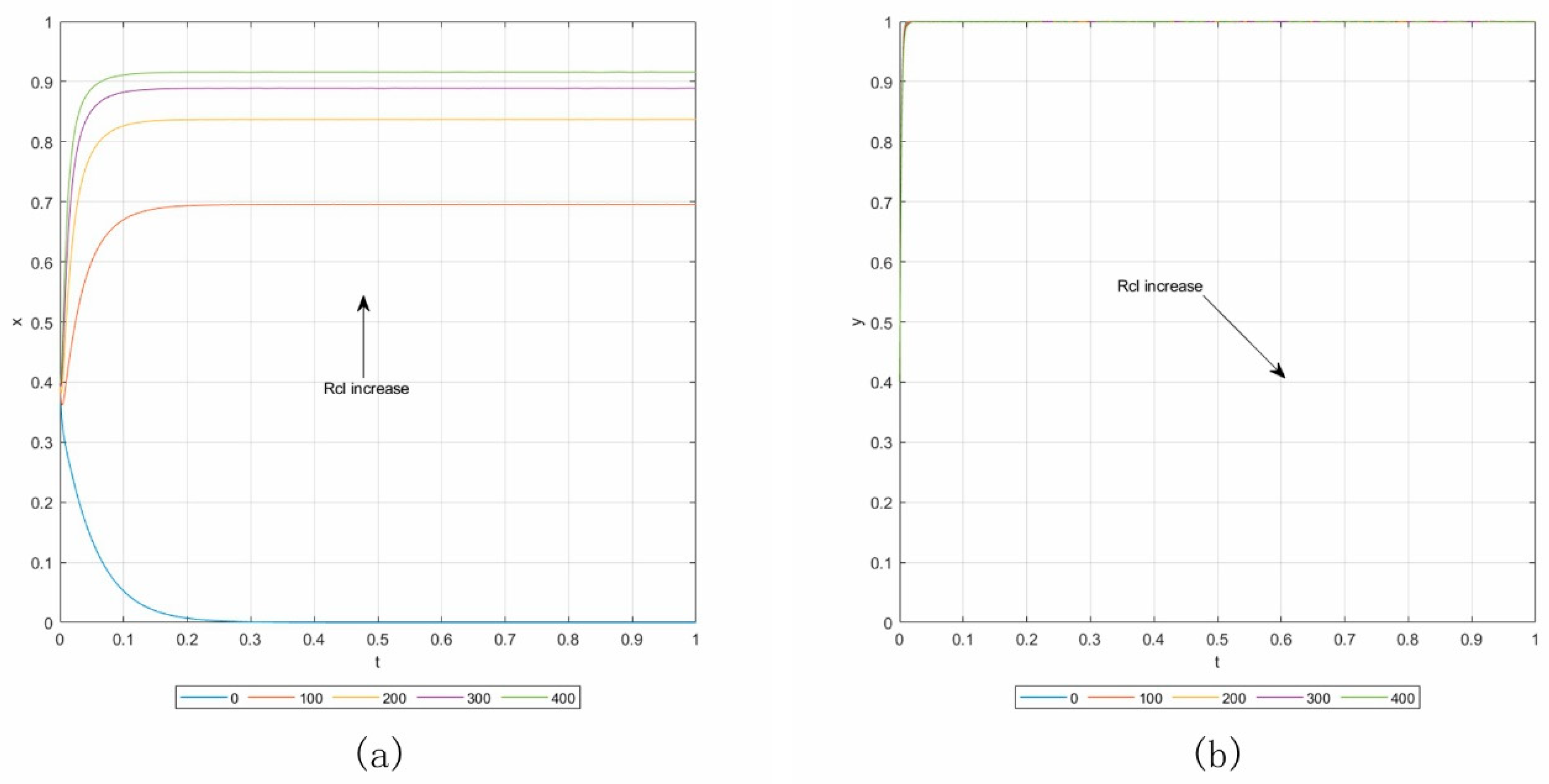
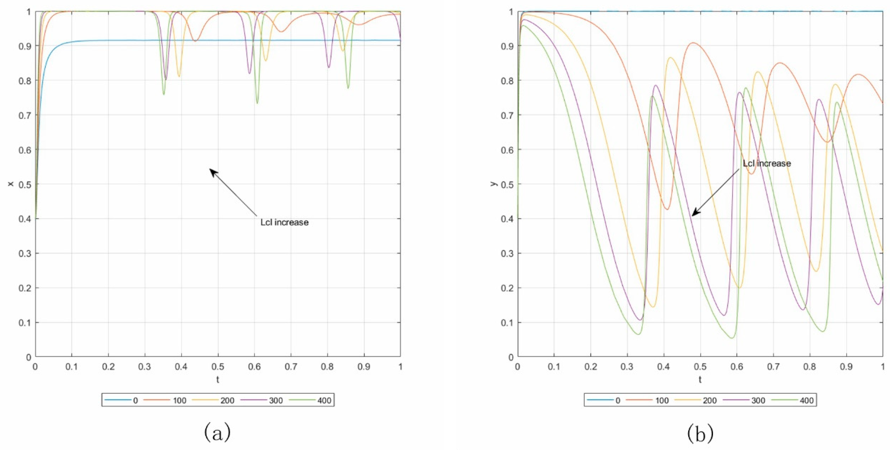
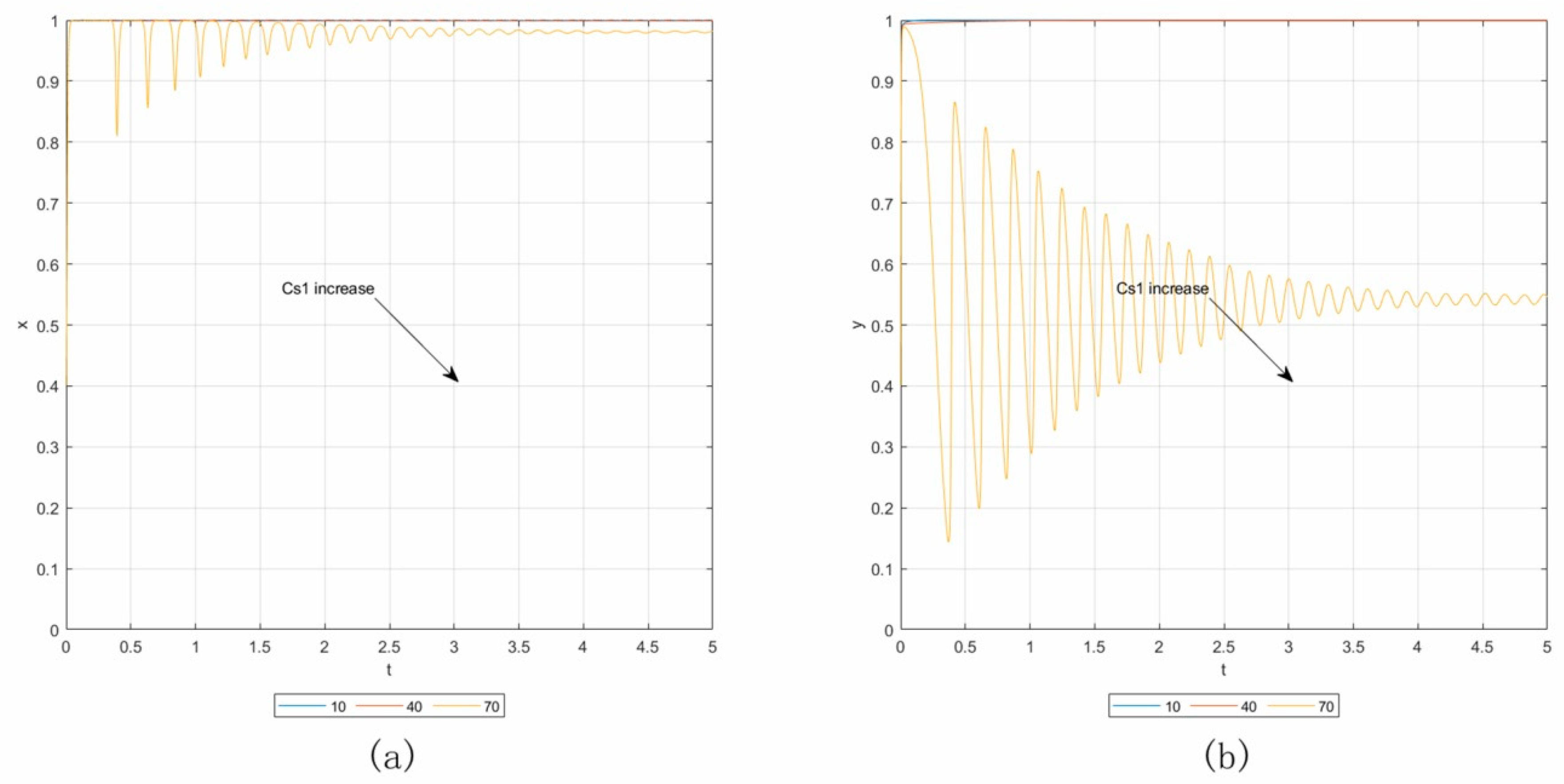
6.3. Influence Analysis of Parameters

In this part, we will further analyze the influence of the parameters related to surety bonds on the behaviors between owners and contractors. Cases 1.1 to 1.4 describe the scenario under a low-penalty unconditional bond, while the analysis under a high-penalty conditional bond is shown in Case 2.1 to 2.7. Here, the starting time is set to 0 and the terminal time to 1 in Cases 1.1 to 2.6. In Case 2.7, the terminal time is set to 5 instead.

Case 1.1. By setting L_cl = 0, C_s2 = 50, and keeping the other parameters consistent with the baseline, the initial point is (0.4, 0.4). Panels (a) and (b) in Figure 2 show the results of the sensitivity analysis, in which R_cl increases from 0 to 320 with an addition of 80. From panel (a), we can see that with an increasing R_cl, contractors are more likely to change its strategy from “default” to “not default”. The more loss caused by the poor reputation in surety bond institutions will help restrict the default behavior of contractors. For panel (b), if R_cl increases, the proportion of owners implementing the “surety bond” strategy will decrease.

Case 1.2. By setting R_cl = 0, C_s2 = 50, and keeping the other parameters consistent with the baseline, the initial point is (0.4, 0.4). Panels (a) and (b) in Figure 3 show the results of the sensitivity analysis, in which L_cl increases from 0 to 320 with an addition of 80. From the results, we can see that the changes of L_cl have almost no influence on the behaviors between owners and contractors.

Case 1.3. By setting R_cl = 0, L_cl = 0, and keeping the other parameters consistent with the baseline, the initial point is (0.4, 0.4). Panels (a) and (b) in Figure 4 show the results of the sensitivity analysis, in which C_s2 increases from 10 to 90 with an addition of 40. From panel (b), when C_s2 increases, the strategies of owners and contractors do not change, but the owners reach the surety bond strategy much more slowly.

Case 1.4. By setting R_cl = 400, L_cl = 200, and keeping the other parameters consistent with the baseline, the initial point is (0.4, 0.4). Panels (a) and (b) in Figure 5 show the results of the sensitivity analysis, in which C_s2 increases from 10 to 90 with an addition of 40. From panels (a) and (b), the increasing C_s2 has a great influence on the strategies of owners and contractors. More contractors are likely to change from the “not default” to “default” strategy, while the owners change from the surety bond to the “not surety bond” strategy.

Case 2.1. By setting L_cl = 0, C_s1 = 70, and keeping the other parameters consistent with the baseline, the initial point is (0.4, 0.4). Panels (a) and (b) in Figure 6 show the results of the sensitivity analysis, in which R_cl increases from 0 to 400 with an addition of 100. In panel (a), it can be seen that with the increasing R_cl, more contractors are likely to change their strategy from “default” to “not default”.

Case 2.2. By setting L_cl = 0, C_s1 = 10, and keeping the other parameters consistent with the baseline, the initial point is (0.4, 0.4). Panels (a) and (b) in Figure 7 show the results of the sensitivity analysis, in which R_cl increases from 0 to 400 with an addition of 100. From panel (a), we can see that with the increasing R_cl, more contractors are likely to change their strategy from “default” to “not default”.

Case 2.3. By setting R_cl = 0, C_s1 = 70, and keeping the other parameters consistent with the baseline, the initial point is (0.4, 0.4). Panels (a) and (b) in Figure 8 show the results of the sensitivity analysis, in which L_cl increases from 0 to 400 with an addition of 100. From panel (a), we can see that when L_cl increases, more contractors are likely to change the “default” strategy to the “not default” strategy. However, the rate of convergence decreases with an increasing L_cl.

Case 2.4. By setting R_cl = 400, C_s1 = 70, and keeping the other parameters consistent with the baseline, the initial point is (0.4, 0.4). Panels (a) and (b) in Figure 9 show the results of the sensitivity analysis, in which L_cl increases from 0 to 400 with an addition of 100. In panel (a), it can be seen that if L_cl increases, the proportion of contractors adopting the “not default” strategy will also increase. Note that the rate of convergence decreases with the increasing L_cl.

Case 2.5. By setting R_cl = 0, C_s1 = 10, and keeping the other parameters consistent with the baseline, the initial point is (0.4, 0.4). Panels (a) and (b) in Figure 10 show the results of the sensitivity analysis, in which L_cl increases from 0 to 400 with an addition of 100. In panel (a), more contractors are likely to implement the “not default” strategy with the increasing L_cl.

Case 2.6. By setting R_cl = 0, L_cl = 0, and keeping the other parameters consistent with the baseline, the initial point is (0.4, 0.4). Panels (a) and (b) in Figure 11 show the results of the sensitivity analysis, in which C_s1 increases from 10 to 70 with an addition of 30. From the results, we can see that the changes of C_s1 have almost no influence on the behaviors between owners and contractors.

Case 2.7. By setting R_cl = 400, L_cl = 200, and keeping the other parameters consistent with the baseline, the initial point is (0.4, 0.4). Panels (a) and (b) in Figure 12 show the results of the sensitivity analysis, in which C_s1 increases from 10 to 70 with an addition of 30. We can see from both panels that the increasing C_s1 will reduce the rate of convergence and change the strategies of owners and contractors. The proportion of contractors implementing the “not default” strategy and the ratio of owners implementing the “surety bond” strategy both decrease with an increasing C_s1.

7. Discussions

This paper analyzes the behaviors between owners and contractors based on dynamic evolutionary game analysis, to discover how to use surety bonds to restrict the default behavior of contractors. Two circumstances are considered—the low-penalty unconditional bond and the high-penalty conditional bond. Though the perfect ESS strategy (not default, not surety bond) cannot be reached in any scenario, some cases still have the good ESS strategy (not default, surety bond). A numerical analysis is also conducted to further explore some parameters’ influence on the behaviors between owners and contractors. The results are discussed as following:

1.

Low-penalty unconditional bond

In the analysis in Section 6.3, R_cl plays a leading role in the influence of the contractors’ strategy choice. More contractors are likely to adopt the “not default” strategy with an increasing R_cl. C_s2 is also an important factor that influences the contractors’ behavior. When R_cl and L_cl are large enough, the decreasing C_s2 will help change the contractors’ strategy from the “default” one to “not default” one. However, if R_cl and L_cl are not large enough, C_s2 has almost no influence on the contractors’ behavior. For the factor L_cl, it has no effect on the strategy choice of contractors, unless combined with R_cl and L_cl.

2.

High-penalty conditional bond

In the analysis in Section 6.3, R_cl still plays a leading role in the influence of the contractors’ strategy choice under a high-penalty conditional bond. With the value of R_cl increasing, more contractors tend to implement the “not default” strategy. Similar to the situation under a low-penalty unconditional bond, C_s1 is also important to influence the contractors’ behavior when R_cl and L_cl are large enough, as the decreasing C_s1 will help the contractors to implement the “not default” strategy with a better rate of convergence. However, different from the situation under a low-penalty unconditional bond, the factor L_cl produces a positive effect on the contractors’ behavior. More contractors want to adopt the “not default” strategy when L_cl increases. However, if the difference between R_cl and L_cl is reduced, the rate of convergence will also decrease.

3.

Comparison

In summary, the high-penalty conditional bond is a preferred method to restrict contractors’ default rather than the low-penalty unconditional bond. The factor R_cl has a more positive effect on the contractors’ behavior under a high-penalty conditional bond. The effect of the cost of surety bonds is almost the same under these two kinds of surety bond, but generally the lower cost of a high-penalty conditional bond will produce more positive effects. The factor L_cl influences the contractors’ behavior positively under a high-penalty conditional bond, while it has almost no influence under a low-penalty unconditional bond.

Based on the discussion above, we hope to give some advice to the policymakers to keep the sustainability of construction markets. The first advice is that the government should put forward the high-penalty conditional bond much more than the low-penalty unconditional bond. It is also necessary to establish the CMCS promoted by the surety bond system. The promotion of surety bonds will be helpful in the establishment of CMCS, as the information exchanged in surety bond systems can ensure that the non-default contractors will obtain more opportunities of construction projects while the default contractors will lose more opportunities in the future. As a result, the values of R_cl and L_cl are positively determined by the development of CMCS, and we should further develop the CMCS to enlarge the values of R_cl and L_cl. Moreover, we need to keep the value of R_cl a little larger than L_cl to reach a more efficient system according to the discussion above. That is to say, the long-term revenue of the “not default” strategy should exceed the long-term loss of the “default” strategy. Furthermore, a larger gap between R_cl and L_cl will help the market to reach the ideal state more quickly. Second, reducing the cost of surety bonds is helpful to the contractors’ “not default” strategy choice only when the CMCS has been established as driven by surety bonds. If the CMCS is not developed well, the cost of surety bonds almost produces no effects on the contractors’ strategy. As a result, CMCS should first be established, and then surety bond institutions need to be subsidized to reduce the cost at the early stage. After the surety bond system has been well developed, some discounts can be provided for the companies with a good reputation.

8. Conclusions

The issue of default in the construction markets is quite important, as it concerns the sustainability of the construction industry. In this paper, we analyzed the mechanism and influential factors of owners’ and contractors’ behaviors under surety bonds, from a new perspective of evolutionary game theory. Another contribution we have made is the dynamic evolutionary game model considering the dynamic factors to solve the problem. The analysis results and the proposed policy suggestions might be suitable for the countries where the CMCS has not been established, such as China. However, there are still some limitations in this paper. First, we just finished the analysis of the behaviors between the owners and the contractors. More parties need to be included through the complex networks and agent models in future work. Second, the analysis in this paper was based on synthetic data, so more real data can be gathered to further evaluate the analysis in the future. Finally, the functions of dynamic factors in this paper are linear. Future studies can explore more types of functions.

References

1. Chava, S.; Jarrow, R.A. Bankruptcy prediction with industry effects. Rev. Finance 2004, 8, 537–569. [Google Scholar] [CrossRef]
2. Tserng, H.P.; Lin, G.-F.; Tsai, L.K.; Chen, P.-C. An enforced support vector machine model for construction contractor default prediction. Autom. Constr. 2011, 20, 1242–1249. [Google Scholar] [CrossRef]
3. Cruz, C.O.; Marques, R.C. Using probabilistic methods to estimate the public sector comparator. Comput. Civ. Infrastruct. Eng. 2012, 27, 782–800. [Google Scholar] [CrossRef]
4. Horta, I.M.; Camanho, A.S. Company failure prediction in the construction industry. Expert Syst. Appl. 2013, 40, 6253–6257. [Google Scholar] [CrossRef]
5. Tserng, H.P.; Ngo, T.L.; Chen, P.C.; Tran, L.Q. A grey system theory-based default prediction model for construction firms. Comput. Civ. Infrastruct. Eng. 2014, 30, 120–134. [Google Scholar] [CrossRef]
6. Wu, W.-W. Beyond business failure prediction. Expert Syst. Appl. 2010, 37, 2371–2376. [Google Scholar] [CrossRef]
7. Kangari, R.; Farid, F.; Elgharib, H.M. Financial performance analysis for construction industry. J. Constr. Eng. Manag. 1992, 118, 349–361. [Google Scholar] [CrossRef]
8. Russell, J.S.; Zhai, H. Predicting contractor failure using stochastic dynamics of economic and financial variables. J. Constr. Eng. Manag. 1996, 122, 183–191. [Google Scholar] [CrossRef] [Green Version]
9. Ng, S.T.; Wong, J.M.; Zhang, J. Applying Z-score model to distinguish insolvent construction companies in China. Habitat Int. 2011, 35, 599–607. [Google Scholar] [CrossRef]
10. Tserng, H.P.; Chen, P.-C.; Huang, W.-H.; Lei, M.C.; Tran, Q.H. Prediction of default probability for construction firms using the logit model. J. Civ. Eng. Manag. 2014, 20, 247–255. [Google Scholar] [CrossRef] [Green Version]
11. Cheng, M.-Y.; Hoang, N.-D.; Limanto, L.; Wu, Y.-W. A novel hybrid intelligent approach for contractor default status prediction. Knowl.-Based Syst. 2014, 71, 314–321. [Google Scholar] [CrossRef]
12. Choi, H.; Son, H.; Kim, C. Predicting financial distress of contractors in the construction industry using ensemble learning. Expert Syst. Appl. 2018, 110, 1–10. [Google Scholar] [CrossRef]
13. You, J.; Chen, Y.; Wang, W.; Shi, C. Uncertainty, opportunistic behavior, and governance in construction projects: The efficacy of contracts. Int. J. Proj. Manag. 2018, 36, 795–807. [Google Scholar] [CrossRef]
14. Nasir, M.K.; Hadikusumo, B.H.W. System dynamics model of contractual relationships between owner and contractor in construction projects. J. Manag. Eng. 2019, 35, 04018052. [Google Scholar] [CrossRef]
15. Zhang, L.; Qian, Q. How mediated power affects opportunism in owner–contractor relationships: The role of risk perceptions. Int. J. Proj. Manag. 2017, 35, 516–529. [Google Scholar] [CrossRef]
16. Liu, J.; Zhao, X.; Li, Y. Exploring the factors inducing contractors’ unethical behavior: Case of China. J. Prof. Issues Eng. Educ. Pr. 2017, 143, 04016023. [Google Scholar] [CrossRef]
17. Lu, W.; Zhang, L.; Zhang, L. Effect of contract completeness on contractors’ opportunistic behavior and the moderating role of interdependence. J. Constr. Eng. Manag. 2016, 142, 04016004. [Google Scholar] [CrossRef]
18. Zhang, S.; Zhang, S.; Gao, Y.; Ding, X. Contractual governance: Effects of risk allocation on contractors’ cooperative behavior in construction projects. J. Constr. Eng. Manag. 2016, 142, 04016005. [Google Scholar] [CrossRef]
19. Kangari, R.; Bakheet, M. Construction surety bonding. J. Constr. Eng. Manag. 2001, 127, 232–238. [Google Scholar] [CrossRef]
20. Awad, A.; Fayek, A.R. Adaptive learning of contractor default prediction model for surety bonding. J. Constr. Eng. Manag. 2013, 139, 694–704. [Google Scholar] [CrossRef]
21. Deng, X.; Ding, S.; Tian, Q. Reasons underlying a mandatory high penalty construction contract bonding system. J. Constr. Eng. Manag. 2004, 130, 67–74. [Google Scholar] [CrossRef]
22. Eaglestone, F.N.; Smyth, C. Insurance under the ICE Contract; Godwin: London, UK, 1985. [Google Scholar]
23. Russell, J.S. Surety Bonds for Construction Contracts; American Society of Civil Engineers (ASCE): Reston, VA, USA, 2000. [Google Scholar]
24. Winston, S.; Ichniowski, T. Procurement: Miller act reforms approved by house. Eng. Newsrev. 1999, 243, 11. [Google Scholar]
25. Bayraktar, M.E.; Hastak, M. Scoring approach to construction bond underwriting. J. Constr. Eng. Manag. 2010, 136, 957–967. [Google Scholar] [CrossRef]
26. Marsh, K.; Fayek, A.R. SuretyAssist: Fuzzy expert system to assist surety underwriters in evaluating construction contractors for bonding. J. Constr. Eng. Manag. 2010, 136, 1219–1226. [Google Scholar] [CrossRef]
27. Awad, A.; Fayek, A.R. A decision support system for contractor prequalification for surety bonding. Autom. Constr. 2012, 21, 89–98. [Google Scholar] [CrossRef]
28. El-Mashaleh, M.S.; Horta, I.M. Evaluating contractors for bonding: DEA decision making model for surety underwriters. J. Manag. Eng. 2016, 32, 04015020. [Google Scholar] [CrossRef]
29. Al-Sobiei, O.S.; Arditi, D.; Polat, G. Managing owner’s risk of contractor default. J. Constr. Eng. Manag. 2005, 131, 973–978. [Google Scholar] [CrossRef]
30. Nash, J. Non-cooperative games. Ann. Math. 1951, 54, 286–295. [Google Scholar] [CrossRef]
31. Smith, J.M.; Price, G.R. The logic of animal conflict. Nat. Cell Biol. 1973, 246, 15–18. [Google Scholar] [CrossRef]
32. Smith, J.M. The theory of games and the evolution of animal conflicts. J. Theor. Biol. 1974, 47, 209–221. [Google Scholar] [CrossRef] [Green Version]
33. Taylor, P.D.; Jonker, L.B. Evolutionary stable strategies and game dynamics. Math. Biosci. 1978, 40, 145–156. [Google Scholar] [CrossRef]
34. Bester, H.; Güth, W. Is altruism evolutionarily stable? J. Econ. Behav. Organ. 1998, 34, 193–209. [Google Scholar] [CrossRef] [Green Version]
35. Dufwenberg, M.; Güth, W. Indirect evolution vs. strategic delegation: A comparison of two approaches to explaining economic institutions. Eur. J. Political-Econ. 1999, 15, 281–295. [Google Scholar] [CrossRef]
36. Naini, S.G.J.; Aliahmadi, A.R.; Jafari-Eskandari, M. Designing a mixed performance measurement system for environmental supply chain management using evolutionary game theory and balanced scorecard: A case study of an auto industry supply chain. Resour. Conserv. Recycl. 2011, 55, 593–603. [Google Scholar] [CrossRef]
37. Wang, G.; Xue, Y.; Skibniewski, M.J.; Song, J.; Lu, H. Analysis of private investors conduct strategies by governments supervising public-private partnership projects in the new media era. Sustainability 2018, 10, 4723. [Google Scholar] [CrossRef] [Green Version]
38. Li, L.; Li, Z.; Jiang, L.; Wu, G.; Cheng, D. Enhanced cooperation among stakeholders in PPP mega-infrastructure projects: A China study. Sustainability 2018, 10, 2791. [Google Scholar] [CrossRef] [Green Version]
39. Zhu, J.; Fang, M.; Shi, Q.; Wang, P.; Li, Q. Contractor cooperation mechanism and evolution of the green supply chain in mega projects. Sustainability 2018, 10, 4306. [Google Scholar] [CrossRef] [Green Version]
40. Hao, C.; Du, Q.; Huang, Y.; Shao, L.; Yan, Y. Evolutionary game analysis on knowledge-sharing behavior in the construction supply chain. Sustainability 2019, 11, 5319. [Google Scholar] [CrossRef] [Green Version]
41. Yang, Y.; Tang, W.; Shen, W.; Wang, T. Enhancing risk management by partnering in international EPC projects: Perspective from evolutionary game in chinese construction companies. Sustainability 2019, 11, 5332. [Google Scholar] [CrossRef] [Green Version]
42. Zheng, L.; Lu, W.; Chen, K.; Chau, K.W.; Niu, Y. Benefit sharing for BIM implementation: Tackling the moral hazard dilemma in inter-firm cooperation. Int. J. Proj. Manag. 2017, 35, 393–405. [Google Scholar] [CrossRef] [Green Version]
43. Du, Y.; Zhou, H.; Yuan, Y.; Xue, H. Exploring the moral hazard evolutionary mechanism for bim implementation in an integrated project team. Sustainability 2019, 11, 5719. [Google Scholar] [CrossRef] [Green Version]
44. Jide, S.; Xincheng, W.; Liangfa, S. Research on the mobility behaviour of Chinese construction workers based on evolutionary game theory. Econ. Res. 2018, 31, 1–14. [Google Scholar] [CrossRef]
45. Pi, Z.; Gao, X.; Chen, L.; Liu, J. The new path to improve construction safety performance in China: An evolutionary game theoretic approach. Int. J. Environ. Res. Public Heal. 2019, 16, 2443. [Google Scholar] [CrossRef] [PubMed] [Green Version]
46. Chen, Y.; Zhu, D.; Zhou, L. A game theory analysis of promoting the spongy city construction at the building and community scale. Habitat Int. 2019, 86, 91–100. [Google Scholar] [CrossRef]
47. Chen, J.; Hua, C.; Liu, C. Considerations for better construction and demolition waste management: Identifying the decision behaviors of contractors and government departments through a game theory decision-making model. J. Clean. Prod. 2019, 212, 190–199. [Google Scholar] [CrossRef]
48. Jide, S.; Xincheng, W.; Liangfa, S. Chinese construction workers’ behaviour towards attending vocational skills trainings: Evolutionary game theory with government participation. J. Differ. Equ. Appl. 2016, 23, 468–485. [Google Scholar] [CrossRef]
49. Shi, Q.; Zhu, J.; Li, Q. Cooperative evolutionary game and applications in construction supplier tendency. Complexity 2018, 2018, 8401813. [Google Scholar] [CrossRef]
50. Xu, X.; Li, Z.; Wang, J.; Huang, W. Collaboration between designers and contractors to improve building energy performance. J. Clean. Prod. 2019, 219, 20–32. [Google Scholar] [CrossRef]
51. Pan, Y.; Deng, X.; Maqbool, R.; Niu, W. Insurance crisis, legal environment, and the sustainability of professional liability insurance market in the construction industry: Based on the US market. Adv. Civ. Eng. 2019, 2019, 1614868. [Google Scholar] [CrossRef] [Green Version]
52. Friedman, D. Evolutionary games in economics. Econ. J. Econ. Soc. 1991, 59, 637. [Google Scholar] [CrossRef] [Green Version]
53. Chen, W.; Hu, Z.-H. Using evolutionary game theory to study governments and manufacturers’ behavioral strategies under various carbon taxes and subsidies. J. Clean. Prod. 2018, 201, 123–141. [Google Scholar] [CrossRef]
54. Fang, Y.; Chen, L.; Mei, S.; Wei, W.; Huang, S.; Liu, F. Coal or electricity? An evolutionary game approach to investigate fuel choices of urban heat supply systems. Energy 2019, 181, 107–122. [Google Scholar] [CrossRef]
Figure 1. Evolution paths of Case 1 to Case 6. (a) Case 1. (b) Case 2. (c) Case 3. (d) Case 4. (e) Case 5. (f) Case 6.
Sustainability 12 09162 g001
Figure 2. Influence of Rcl in Case 1.1. (a) Influence on contractors. (b) Influence on owners.
Sustainability 12 09162 g002
Figure 3. Influence of Lcl in Case 1.2. (a) Influence on contractors. (b) Influence on owners.
Sustainability 12 09162 g003
Figure 4. Influence of Cs2 in Case 1.3. (a) Influence on contractors. (b) Influence on owners.
Sustainability 12 09162 g004
Figure 5. Influence of Cs2 in Case 1.4. (a) Influence on contractors. (b) Influence on owners.
Sustainability 12 09162 g005
Figure 6. Influence of Rcl in Case 2.1. (a) Influence on contractors. (b) Influence on owners.
Sustainability 12 09162 g006
Figure 7. Influence of Rcl in Case 2.2. (a) Influence on contractors. (b) Influence on owners.
Sustainability 12 09162 g007
Figure 8. Influence of Lcl in Case 2.3. (a) Influence on contractors. (b) Influence on owners.
Sustainability 12 09162 g008
Figure 9. Influence of Lcl in Case 2.4. (a) Influence on contractors. (b) Influence on owners.
Sustainability 12 09162 g009
Figure 10. Influence of Lcl in Case 2.5. (a) Influence on contractors. (b) Influence on owners.
Sustainability 12 09162 g010
Figure 11. Influence of Cs1 in Case 2.6. (a) Influence on contractors. (b) Influence on owners.
Sustainability 12 09162 g011
Figure 12. Influence of Cs1 in Case 2.7. (a) Influence on contractors. (b) Influence on owners.
Sustainability 12 09162 g012