The Impact of Monetary Policies on the Sustainable Economic and Financial Development in the Euro Area Countries

Abstract

One of the responses of the monetary policies of central banks to the sustainable development on financial markets, which also affected other markets and economic growth, is the role of non-standard monetary policies, referred to as quantitative easing in the form of Asset Purchase Programme. In this paper, the following main research problem was addressed: How can the Asset Purchase Programme help the European Central Bank fulfill its mandate of supervising the financial stability and financial development? Based on this, we formulated the main objective: to identify the impact of monetary policies on the dynamics of financial markets development, labor markets, and the markets for goods and services. As part of the applied methodology, the impact of the quantitative easing on the government bond yields curve was based on an indirect assessment using the seemingly unrelated regression model, considering the use of parameters from the functional benchmark form. Through the vector error correction model, another additional impact of the application of the monetary policy mechanisms on selected indicators of the considered markets was identified. The relationship between financial markets and economic growth was determined on the basis of the two-stage least square model using endogeneity control instruments. Applying the changes identified by the above models allowed us to determine the expected change in the rate of growth of the aggregate output of the euro area countries. Based on our results, we found out that Asset Purchase Programme had an impact on the growth of government bond yields issued by euro area countries, on lowering the risk rate on corporate bond markets, and increasing the nominal value of shares. In addition, growth in inflation and a decline in interest rates were affected. Finally, the European Central Bank (ECB)’s non-standard monetary policies have positively affected and stimulated the labor market and development in goods and services markets, referred to the sustainable financial development.

1. Introduction

The concept of sustainable development is based on three known pillars: sustainable economic growth, social inclusion, and environmental protection have been recognized as fundamental in the development processes in all the EU countries, according The Agenda 2030 for sustainable development. The European Central Bank as the supreme institution of the EU has a clear mandate—sustaining financial development and price stability in the EU, using its monetary policies and mechanisms.

Quantitative easing is characterized as a monetary policy of redemption of assets funded by the central bank’s provisions, which was first introduced by [1,2] to name the Bank of Japan policy conducted between 2001 and 2006. Many central banks have used outright purchases as part of their monetary policies. It has been employed by the Federal Reserve Board, the Bank of England, and the Bank of Japan. Open market operations are a core instrument of central banks even in standard times.

The central bank intervention, called quantitative easing, took an important place in three major economies (Japan, the US, and England) and in the European Monetary Union (EMU), which brought about differences and distinctive patterns for each. The most significant difference between each country’s quantitative easing was, according to [3], that the Fed’s buy-back and the Bank of England operations were not designed to address the liquidity problem of the banking system (rather focused on increasing asset prices/returns), which is related to the fact that the European Central Bank (ECB) and the Bank of Japan were economies with a stronger focus on the banking sector, while in England and the US, the securities markets are relatively more dominant [4]. According to [5], the relative increase in the size of the banking system against the private sector’s securities market is associated with greater systemic risks and lower economic growth.

The impact of higher liquidity on economic system is also described by [6], primarily focusing on central bank purchases raising asset prices and, if asset prices are higher, lowering borrowing costs and encouraging an increase in consumption and investment. In contrast, analysis by [7,8] can conclude that while quantitative easing (as a central bank’s liquidity-increasing tool) has a significant impact on financial markets and partly on interest (and thus price) on government bonds, it is clear that it is best to understand the transfer of these effects to the economy, and [9] has also addressed this issue in the United Kingdom. Authors [10] propose that the efficiency of the monetary system be identified by an integrated general model of the ultimate goal that most stakeholders could agree on—nominal GDP growth. On the basis of these findings, we proceeded to a smaller adjustment and selected GDP aggregates and in our study, investigated the impact of monetary policy on them.

Authors [11] argue that both quantitative easing and other non-standard (or non-interest-rate) operations changing the composition of the central bank’s assets in its financial statements mainly affect the interest rate, specifically the spread of the money market rather than through the effects of quantity in money demand conditions, assuming that these effects have some delay on impact. However, [12] believe that central bank asset growth is not helpful in restoring economies from crises and is therefore unlikely to become attractive as a major monetary instrument. Authors in [13], who earlier expressed that the effectiveness of quantitative easing is still open to considerable doubts, were similarly interested. In addition, [14] argues that quantitative easing will lead to the control of the common monetary policy by national fiscal policies. Author [15] argues that the simultaneous budgetary consolidation in 2011–2013 has led to a decline in real GDP in the monetary union of around 1% per year. In addition, [16] estimates that public finance savings affects the reduction in bond purchases. Thus, the stimulus effect of central bank budget interventions against the 2009 recession was more or less offset by austerity fiscal policy. This, moreover, is most likely to have contributed to the reuse of this type of instrument within the ECB’s strategies.

The main goal of our study is to identify the impact of monetary policy instruments on the dynamics of financial market development, labor market, and the markets for goods and services, examine and provide a characterization of the dynamic economic interactions between the important macroeconomic, financial, and market indicators, using the methodology of modeling. Special attention is devoted to the effects of Asset Purchase Programmes of the ECB on the economic and financial development in the euro area countries, investigated by means of four research questions, in the context of encourage sustainable development. Our findings demonstrated the important economic effects on financial market development, labor market, and the markets for goods and services, during the examined period.

Based on the mentioned research problems and findings our study focuses on the impact of selected instruments of the European Central Bank (ECB) in its non-standard monetary policy on the economic growth dynamics of euro area countries, focusing on quantitative easing—Section 1 and Section 2. The methodology of our analyses was based on the analysis of empirical studies, the application of existing models (the seemingly unrelated regression (SUR) model, vector error correction model (VECM) models, and the growth two-stage least squares (2SLS) model, specified in Section 3 and Section 4), sample characteristics of the data used for the period under review 3.Q. 2009–3.Q. 2018 and 2000–2018 in the Section 3 and Section 4. Results and discussion are presented in Section 4 and Section 5 while examining the primary concentration of ECB quantitative easing mechanisms on average securities yields and the effects of these yields on financial markets and sustainable economic growth in euro area countries. Then finally in the conclusion we summarize the implications in a broader context.

2. Literature Review—The ECB, Its Monetary Policy at a Time of Financial Crisis and Now

Throughout the crisis, the ECB has used a number of strategies and mechanisms to help promote consumption and reach inflation targets. However, most of the central bank’s instruments in response to the financial crisis already existed within the Bank’s operational frameworks in the pre-crisis period [11]. It is just about extending the current operations of the central banks of the above mentioned entities. The combination of a wide range of measures could have led to different interactions between mechanisms. Authors [17] recommend coordination of unconventional and conventional monetary policy measures, according to the authors, the short-term interest rate should respond to inflation (central bank inflation targets), while purchases of long-term securities (debt) should respond to output (country production). Quantitative easing can certainly affect the real economy through exchange rates and net exports [18]. In addition, such an unconventional policy helps to keep the securities yield spreads steady [19]. According to [20], it is then appropriate to use quantitative easing in the case of a base rate of less (or equal) to zero. In addition, as the EMU is still in a liquidity trap, there is no limit to the number of government bonds redeemed by the ECB without starting inflation [21]. Indeed, such a situation still exists within the EMU. In addition, [22] is convinced that a potential bond shortage in the European Monetary Union exists throughout the duration of the Assets Purchase Programme (APP). Many experts and authors discussed the effects of APP worldwide, and in ECB’s working papers. Authors [23] examined the effects of the APP on the financial markets in the euro area and found the effects in bond yields and spread reduction to decreasing risks for portfolio rebalancing in all countries.

The ECB’s APP includes a number of instruments, some of which have already been completed. The SMP—Securities Market Programme, CBPP I and CBPP II—Covered Bond Purchase Programmes are closed. According to [24] in the case of SMP, the answer to the downturn in some secondary markets for government bonds was to improve the functioning of the transmission mechanism by providing liquidity in the non-functioning segments of the bond markets. In the case of CBPP, it was the renewal of the covered bond market, which is the primary source of funding for EMU banks, by supporting the decline in money market interest rates and simplifying funding conditions for credit institutions and businesses.

We will then move on to the characteristics of the ECB’s current running mechanisms. CBPP III worked on the same principle as previous programmes. ABSPP—Asset Covered Bond Purchase Programme launched to promote the direct provision of bank loans through providing the possibility of packing existing loans in Asset-Backed Securities (ABS) in packages they may sell to the ECB. This would give banks free capital for new lending [25]. CSPP—Private sector redemption Programme, which means the purchase of euro-denominated bonds issued by non-bank entities located in the euro area. Details of the corporate bond structure were not reported, but the ECB said that the programme did not lead to higher purchases under APP. This indicates that bond purchases will be made to support existing programmes [26]. PSPP—Public sector redemption Programme (securities) involving government bonds, agencies, international organizations, and development banks located in monetary union [27]. In addition to the APP Programme, we were still thinking about the impact of the underlying money market interest rate, which is one of the central bank’s primary instruments. The final mechanism to be evaluated is TLTROs—targeted longer-term refinancing operations, which are characterized as Eurosystem operations, providing financing to credit institutions, and providing liquidity in market segments.

The central bank affects only the determination of short-term returns, and long-term yields from securities holdings are determined on the basis of demand and supply on the stock markets. This impact of monetary policy instruments on yield levels of securities and other markets needs to be divided in our designed models and modeling (specified in the Section 3). The difference between long-term and short-term returns on securities is discussed by [28], and others.

3. Materials and Methods

3.1. Methodology

The main objective of this study is to identify the impact of ECB non-standard monetary policies on the dynamics of financial markets development and economic development across EMU countries through selected macroeconomic, market, and financial variables.

The findings of research studies focused on the tools of monetary policies stimulated as to create these research questions, which we formulated as follows. The research problem of this work is whether the individual Programmes (non-standard policies) of the ECB were an effective tool for influencing and sustaining the financial markets, goods, and services markets, or the EMU labor market. The following research questions were formulated in the context of the specific characteristics of the elements involved in the subject matter:

How can the Asset Purchase Programme help the ECB to fulfill its mandate to supervise the financial stability and development? Can this Programme help the ECB to support faster or sustainable growth and job creation in Europe?

Subsequently, we formulated these more detailed research questions (RQ):

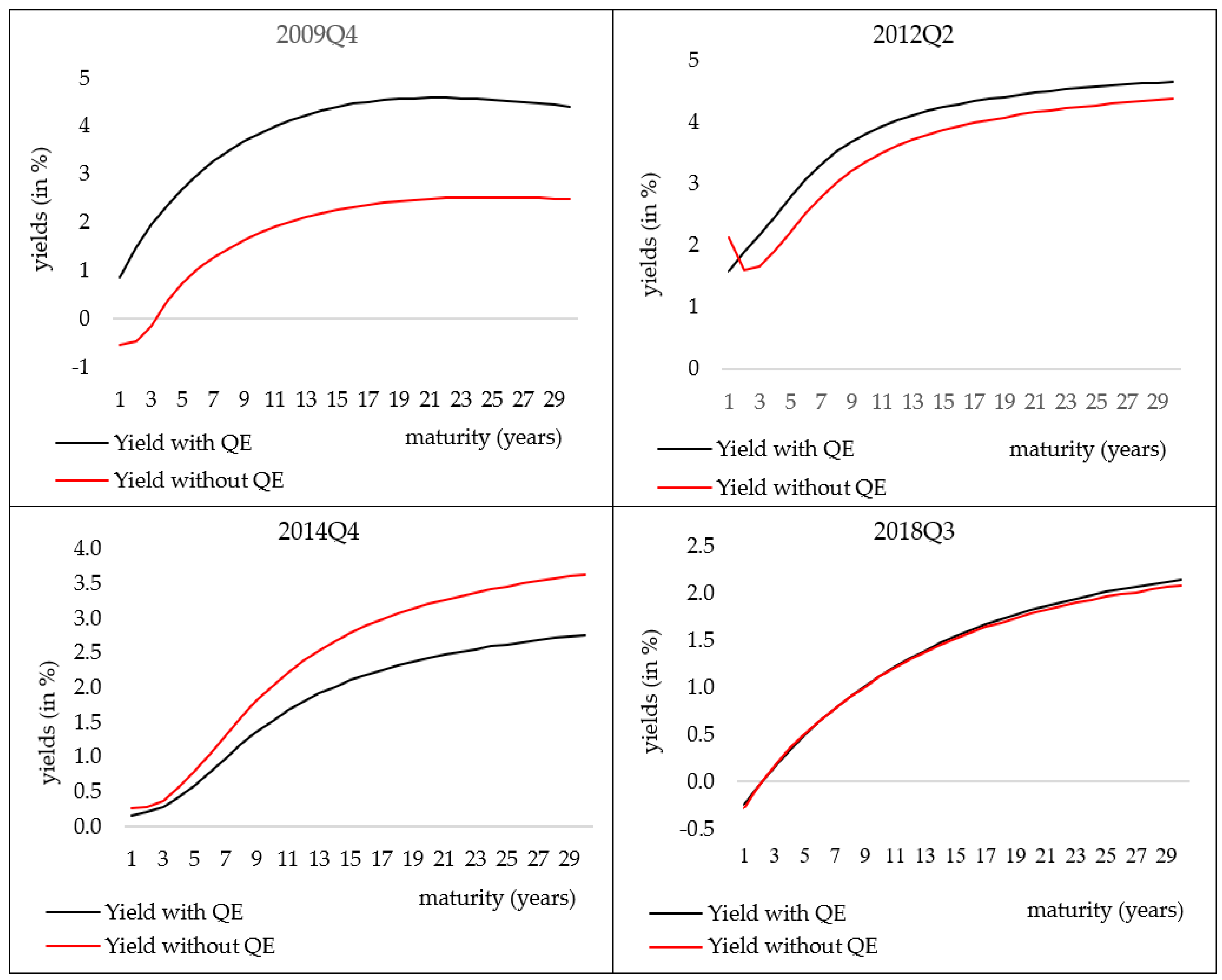
• Research question 1 (RQ1). What will be the impact of the non-standard monetary policy instruments of the ECB in the form of Asset Purchase Programme (or Quantitative easing—QE) mechanisms on zero-coupon yield curve spot rate of all EMU government bonds?
• Research question 2 (RQ2). What additional impact will these instruments have on the financial markets, on the goods and services markets, respectively, or on the labor market?
• Research question 3 (RQ3). How did these policies affect GDP change rates?
• Research question 4 (RQ4). How does the policy effectiveness change over the time?

Based on the methodology and work of [13,29,30], we consider four parameters zero-coupon yield curve rate of all EMU government bonds, in which we will determine the impact of the selected set of variables via the seemingly unrelated regression (SUR) model using the Generalized Least Squares (GLS) estimator. The given curve parameters are level (L), slope (S), first curvature factor (C1), and second curvature factor (C2). The model equation has the following form:

$${\mathrm{Y}}_{\mathrm{t}} = \mathsf{\alpha } + \mathsf{\rho }{\mathrm{Y}}_{\mathrm{t}-4} + \mathsf{\theta }{\mathrm{X}}_{\mathrm{t}} + {\mathsf{\epsilon }}_{\mathrm{t}}$$

(1)

where Y represents the four yield curve parameters, the X matrix of macroeconomic variables, where we consider inflation (HCIP), real activity index (RAI), unemployment (UNEM), interest rate (IR), ratio of public debt to aggregate production (DEBT), effective exchange rate (EER), business confidence index (BCI), weighted retail sales of main trade partners (SALES), index of financial returns (INDEX), Fed funds rate (FED), EURIBOR spread (E_SPREAD), measure of real money and traveler’s checks, and demand deposits (M1). The selection of variables into individual partial equations was done by step-wise technique. This model determines the expected impact of QE on the government bond yield curve indirectly, that is through a model error.

The resulting parameters were converted into yield curves using [31] functional form:

$${\mathrm{y}\left(\mathsf{\tau }\right) = \mathsf{\beta }}_1{+ \mathsf{\beta }}_2\left(\frac{1-{\mathrm{e}}^{-{\mathsf{\tau }\mathsf{\lambda }}_1}}{{\mathsf{\tau }\mathsf{\lambda }}_1}\right){+ \mathsf{\beta }}_3\left(\frac{1-{\mathrm{e}}^{-{\mathsf{\tau }\mathsf{\lambda }}_1}}{{\mathsf{\tau }\mathsf{\lambda }}_1}-{\mathrm{e}}^{-{\mathsf{\tau }\mathsf{\lambda }}_1}\right){+ \mathsf{\beta }}_4\left(\frac{1-{\mathrm{e}}^{-{\mathsf{\tau }\mathsf{\lambda }}_2}}{{\mathsf{\tau }\mathsf{\lambda }}_2}-{\mathrm{e}}^{-{\mathsf{\tau }\mathsf{\lambda }}_2}\right)$$

(2)

where y (τ) is perceived as yield of the bond with maturity τ, β₁ represents the parameter L, β₂ is S, β₃ captures C1, β₄ expresses C2, and parameters λ₁ and λ₂ are characterized as the rate of exponential decay.

Other additional QE impacts on goods and services markets, financial markets, and the labor market were determined on the basis of [32], respectively an extension to determine the impact of QE on changes in other financial indicators based on [33,34]. A vector error correction model (VECM) considering co-integrated variables was used to determine this effect. The choice of the appropriate model type and the number of delays considered was based on the Johansen’s co-integration test [35]. The model equation used then has the following relationship:

$$\Delta {\mathrm{MB}}_{\mathrm{t}} = {\mathsf{\kappa }}_1 {\mathrm{ECT}}_{\mathrm{X}} + {\displaystyle \sum }_{\mathrm{p} = 1}^{\mathrm{r}}{\mathsf{\xi }}_{1,\mathrm{p}} \Delta {\mathrm{MB}}_{\mathrm{t}-\mathrm{p}}+{\displaystyle \sum }_{\mathrm{q} = 1}^{\mathrm{r}}{\mathsf{\Phi }}_{1,\mathrm{q}} \Delta {\mathrm{X}}_{\mathrm{t}-\mathrm{q}}+ {\mathsf{\epsilon }}_{1,\mathrm{t}}$$

(3)

$$\Delta {\mathrm{X}}_{\mathrm{t}} = {\mathsf{\kappa }}_2 {\mathrm{ECT}}_{\mathrm{X}} + {\displaystyle \sum }_{\mathrm{p} = 1}^{\mathrm{r}}{\mathsf{\xi }}_{2,\mathrm{p}} \Delta {\mathrm{MB}}_{\mathrm{t}-\mathrm{p}}+{\displaystyle \sum }_{\mathrm{q} = 1}^{\mathrm{r}}{\mathsf{\Phi }}_{2,\mathrm{q}} \Delta {\mathrm{X}}_{\mathrm{t}-\mathrm{q}}+ {\mathsf{\epsilon }}_{2,\mathrm{t}}$$

(4)

with error correction term (ECTX) in type 1 being considered as

$${\mathrm{ECT}}_{\mathrm{X}} = {\mathrm{MB}}_{\mathrm{t}-1} + \mathsf{\Psi }{\mathrm{X}}_{\mathrm{t}-1}$$

(5)

respectively (for type 2) as

$${\mathrm{ECT}}_{\mathrm{X}} = {\mathrm{MB}}_{\mathrm{t}-1} + \mathsf{\Psi }{\mathrm{X}}_{\mathrm{t}-1} + \mathrm{h}$$

(6)

where MB is understood to be a change of monetary base due to QE; p and q represents lag order of difference of QE (MB) and other selected variable (X), respectively; r represents specified maximum delay; h represents inverse constant of co-integration equation; and κ, ξ, Φ, and Ψ are coefficients.

As a final step, we have developed a growth model designed by [36], which uses the two-stage least squares (2SLS) with instrumental variables to control endogeneity. The model is in the shape of

$$\Delta {\ln \left(\mathrm{GDPpc}\right)}_{\mathrm{t}} = \mathsf{\alpha } + \mathsf{\beta } {\mathrm{X}}_{\mathrm{t}}+ \mathsf{\omega } {\mathrm{FIN}}_{\mathrm{t}-4} + {\mathsf{\epsilon }}_{\mathrm{t}}$$

(7)

where GDP_pc represents gross domestic product per capita, X is a matrix of variables adjusted to a natural logarithm consisting of a seasonal delay of the dependent variable (GDPpct-4) capturing the Solow–Swan convergence effect, investment rate (I/GDP), openness of the economy (OPEN), secondary education (SECON) population share, government expenditure rate (GOV). The last variable of the model is the instrument of the seasonally delayed and logarithm financial variable (FINt-4), which in each model represents liquid liabilities (LLY), private credit (PRIV), bank assets (BANK), and stock market capitalization (SMC). Instruments are, seasonal delay (FINt-8), index of market regulation, index of market credit regulation and index of the degree of judicial independence. The final impact of QE on the change in aggregated country production was determined by the expected changes in some variables due to APP (based on previous models). These variables included GOV (due to changes in government bond yields), MB volume, and possibly the amount of investments based on the above-mentioned work of [36], where we determine the changes in investment rates based on the model:

$$\ln {\left(\frac{\mathrm{I}}{\mathrm{GDP}}\right)}_{\mathrm{t}}{ = \mathsf{\alpha } + \mathsf{\beta } \mathrm{X}}_{\mathrm{t}}{ + \mathsf{\omega } \mathrm{FIN}}_{\mathrm{t}}$$

(8)

where one change from the previous model is a change in variables belonging to the calculating logarithm matrix X, which consists of aggregated output (GDP), interest rate (IR), government spending rate (GOV), and openness of the economy (OPEN). In this case, we do not include stock market capitalization (SMC) among the financial variables considered. Moreover, in this case, the financial variable was instrumented by all other predictors.

The above analyses were processed by software Programme R (v3.4.3), respectively its extension RStudio (in 1.1.442).

3.2. Data

Within the above-mentioned methodology, we work with a dataset that contains a wide range of indicators capturing the situation on the financial markets and the labor market, respectively, and other macroeconomic indicators (accessible data during this research).

The first model (SUR) consists of EMU data as a whole across the time period of APP Programmes, from the third quarter of 2009 until the penultimate period of the programme (the third quarter 2018). Data from the four parameters (L, S, C1, and C2) of zero-coupon yield curve spot rate of all EMU government bonds were obtained from the ECB database. We can divide the independent variables from the first model into five logical structures: inflation, activity, policy, foreign trade, and financial indicators. Inflation in the data used is considered to be the harmonized index of consumer prices (HICP). Activity indicators include the unemployment indicator (UNEM) and the real activity index (RAI), which is constructed through changes in indexes of deflated turnover of sales in retail trade (except for motor vehicles), volume index of production in industry, volume index of production in services and economic sentiment index on the basis of the first component of the principal component analysis. In the policy category we include the interest rate (IR) and the debt to GDP ratio (DEBT). Foreign trade consists of variables such as effective exchange rate (EER), business confidence index (BCI), and weighted (based on proportion of trade) retails sales of main trade partners (SALES). The following variables are listed in the last category. The variable labeled FED presents the funds rate of the Federal Reserve. Stock price (INDEX) is constructed with the first principal component of the average open stock price during the observed timeframe, considering the indexes EUROSTOXX, DAX, and CAC. The EURIBOR spread (E_SPREAD) is defined as the difference of 3-month euro interbank offered rate and overnight interest rate swaps. The last variable considered is M1 (M1) type monetary aggregates.

The VECM model analyses were also applied to aggregated EMU data over a defined period. The volume of QE in the APP form is seen in these models as a change in the monetary base (MB). The IP variable captures the volume index of production in industry. In one of the models, we also consider the current level of capacity utilization in industry (ICU). The SCSD variables are short-term credit spreads, which are characterized as the difference between the weighted short-term bond yield of the selected indexes and the aggregated two-year EMU countries government bond yields. The medium-term credit spread (MCSD) variable is similar to the SCSD but uses the medium-term bond yield and the five-year EMU countries government bond yields. Other variables used within these models were defined above.

The model (2SLS) captures the evolution of EMU aggregated data from the beginning of 2000 to the third quarter of 2018. The I/Y variable expresses the rate of investment in terms of production size, in which case we defined investments as gross fixed capital formation. The openness indicator of EMU economies (OPEN) was determined as the ratio of the sum of exports and imports to aggregated production. We perceive the proportion of population with completed secondary education (SECOND) as a measure of human capital. The public expenditure indicator (GOV), expressed in terms of the GDP, was also used. The first used financial variable within this model is defined as liquid liabilities (LLY), which are perceived as M2 monetary aggregates and are expressed in terms of the GDP. Private credit (PRIV) is understood as credit provided by the banking sector and other intermediaries to the private sector of the economy, and this variable is also expressed in relation to the GDP. The variable labeled BANK represents the total amount of financial assets of the banking sector. The last financial variable under consideration is stock market capitalization (SMC), representing value of listed shares to GDP.

All of the above data comes from the Statistical Office of the European Union (Eurostat), the European Central Bank (ECB), the OECD, the Federal Reserve Economic Database, and the Bank for International Settlements (BIS) total credit statistics database.

4. Results

4.1. Design the Seemingly Unrelated Regression (SUR) Model

The selection of suitable predictors within each of the four equations of the constructed model was performed by step-wise technique within GLS models containing the entire set of predictors considered, determined sequentially for each partial dependent SUR model separately. However, in the context of the SUR concept, also considering correlated error terms models, the significance of some independent variables were not demonstrated again. Even variables such as aggregated (and weighted) retail sales of main EMU member’s trade partners (sales), respectively a composite variable consisting of multiple stock indexes (index), showed no significance in all cases. Inflation (inf) measured by HCIP has reached the expected positive effect on the level and in addition to the second curvature effect, which is related to the fact that bond prices are included in the CPI to determine inflation. On the contrary, real activity index (rai) affects yield returns of government bonds, i.e., a decline in the level of gradual growth, which is more intense in the short run. While in the case of the second indicator of activity—unemployment (unem), we consider only the growth of the slope within the results. From the effects of the interest rate predictor (i), respectively of its impact, the above Breuss (2016) opinion on the possibility of functional QE application was confirmed only if the interest rate is negative, correspondingly converges to zero. The debt-to-aggregate ratio (debt) does not surprisingly affect the level (L) or slope (S) of the yield curve, but its impact was significant for the first and second curvature factor, with growth (expected) lowering the rate of return on government bonds with higher maturity. The effective exchange rate (eer) was expected to reduce the level of bond yields, but in the case of slope this was the opposite. The same contradiction has been found in both curvature factors. The overall yield curve decreased more significantly in the case of effective exchange rate growth, although bonds with higher maturities yielded a higher rate of return (against the level of curve), while this increase gradually lost intensity. The Business confidence index (bci), we considered only within the level and slope based on the step-wise selection of predictors within the compiled SUR model, with this index increasing the level of government bond yields, with their gradual decline. Subsequently, we focus on the independent variable Fed funds rates (fed), which affects the growth of government bond yields, causing a slowdown in yield changes in the short term due to their maturity. The EURIBOR spread variable (Euribor), resp. the difference between the three-month EURIBOR and the Overnight Interest Rate Swaps is characterized by an impact on the significant decline in government bond yield levels. The last significant predictor considered is the ratio of M1 monetary aggregates and euro area aggregate output (m1), which affects all components of the yield curve. Increasing the share of liquid money derivatives affects the growth of the level and second curvature factor, while the other has the opposite. Thus, M1-type money aggregates increase yield levels but influence their decline in view of the rising maturity, with the pace of this decline increasing in the long run. As mentioned above, this model determines the expected impact of QE on the government bond yield curve indirectly, i.e., through a model error. Figure 1 shows the actual values and expected values of the model (representing the situation without applying a non-standard monetary policy in the form of QE) in selected time periods of the observed period, which are based on Svensson’s benchmark term structure model converted to the yield curve for a given year of maturity from 1 to 30 years.

The choice of time slots was not accidental, as the fourth quarter of 2009 represents the period immediately following the start of the expansion of the use of non-standard monetary policy in the form of a QE to the APP Programme (used to mitigate the effects of the financial crisis), specifically the CBPP I. mechanism. The critical period of using the APP Programme has provided a significant impact on corporate bond markets, creating a reduced demand for government bonds. This finding, together with the fact that the introduction of the first mechanisms from APP gave bad signals to the markets, which led to an increase in government bond yields; hence, the risk of holding them. The second quarter of 2012 is the end of the first APP (CBPP I and SMP) package and the start of the second package (CBPP II). This period was mainly related to the calming of the markets, but still to negative expectations. That is why the effect of QE on government bond yields had a slightly decreasing effect on high-maturity bonds. Reducing the spread between the yields of individual situations (actual and expected not using APP) suggests that the effect of the instruments themselves on the bond markets is decreasing and the question of their re-use has arisen. The third period is immediately following the start of the buy-in through the third APP and non-standard open market operations (CBPP III, ABSPP, PSPP, CSPP, and TLTRO I and II). The results show that these instruments have had a greater impact on higher maturity bonds, which is also related to the fact that developments and expectations on European markets have started to improve over this period, and this effect on yield has been multiplied by the use of mechanisms. While the PSPP mechanism was applied directly to the purchase of government bonds during this period, its effect was more pronounced than that of other programmes intended for corporate securities markets. We also assessed the impact in the last observed period (the penultimate period of APP use). Based on the comparison of both situations (actual and considered non-utilization of APP), we are of the opinion that in this period QE has only a minimal effect on government bond yields (or inversely on corporate bonds) and its use (even with regard to the amount of money spent) is no longer needed.

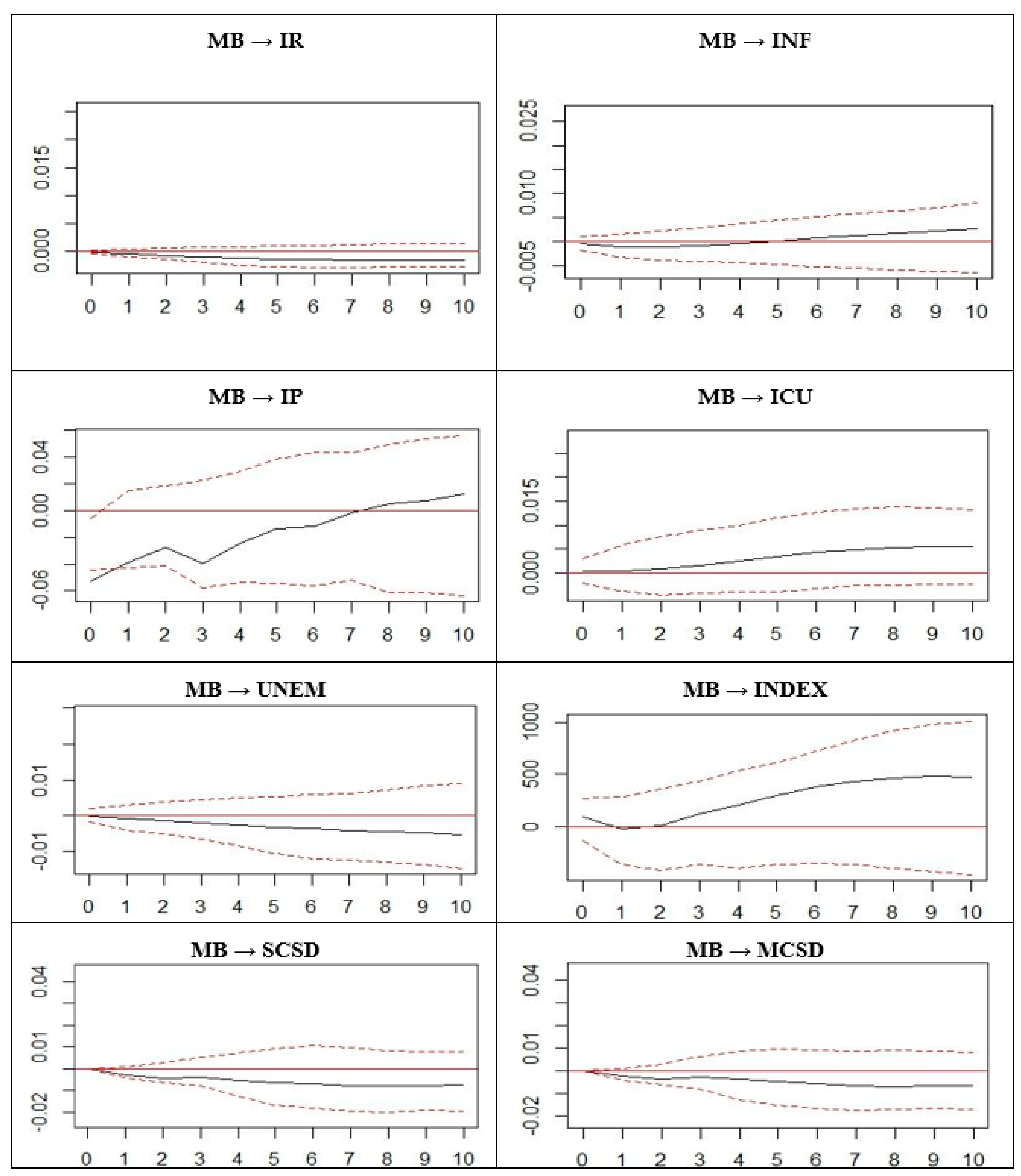
4.2. The Effects of Quantitative Easing (QE) on the Euro Area Countries’ Economies

The next step is to identify other additional effects of QE on the economy of the Euro area countries (perceived as a whole). All conditions were met, and the results of their testing are shown in

Table A2. Results of Vector Error Corrected model.

MB&IR			MB&INF
Cointegration Equation			Cointegration Equation
MB(t−1)	1.0000		MB(t−1)	1.0000
	(0.0000)			(0.0000)
IR(t−1)	8.6035		INF(t−1)	−1.9308
	(3.1076)			(0.8946)
	[8.94e−3] ***			[0.0378] **
(Intercept)	−0.0818		(Intercept)	1.9705
	(0.0540)			(0.7911)
	[0.1389]			[0.0176] **
ECM for cointegrated series			ECM for cointegrated series
	Δ MB	Δ IR		Δ MB	Δ INF
ECT	−0.0639	−0.0085	ECT	−0.0107	−0.0304
	(0.0386)	(0.0048)		(0.0210)	(0.0072)
	[0.1068]	[0.0853] *		[0.6136]	[1.63e−4] ***
∆ MB(t−1)	0.5498	−0.0125	∆ MB(t−1)	0.5532	−0.1078
	(0.1476)	(0.0184)		(0.1681)	(0.0581)
	[6.86e−4] ***	[0.5014]		[2.28e−3] ***	[0.0720] *
∆ IR(t−1)	0.6174	0.6488	∆ INF(t−1)	0.0065	0.1120
	(0.9202)	(0.1145)		(0.4747)	(0.1639)
	[0.5067]	[2.13e−6] ***		[0.9892]	[0.4989]
Q1	0.0025	-0.0004	Q1	0.0044	0.0011
	(0.0029)	(0.0004)		(0.0038)	(0.0013)
	[0.3945]	[0.3242]		[0.2547]	[0.4032]
Q2	−0.0014	0.0001	Q2	0.0004	0.0023
	(0.0030)	(0.0004)		(0.0040)	(0.0014)
	[0.6436]	[0.8040]		[0.9209]	[0.1094]
Q3	−0.0001	−0.0002	Q3	0.0018	−0.0021
	(0.0029)	(0.0004)		(0.0041)	(0.0041)
	[0.9727]	[0.6202]		[0.6633]	[0.6117]
R2	0.3531	0.4461	R2	0.3273	0.6607
Adj. R2	0.2722	0.3769	Adj. R2	0.2432	0.6183
AIC	−15.5846	−15.6390	AIC	−15.3337	−15.3521
BIC	−15.0006	−15.1280	BIC	−14.7498	−14.8412
Cross-equation covariance matrix:			Cross-equation covariance matrix:
	MB	IR		MB	INF
MB	2.34e−3	−2.16e−6	MB	2.35e−3	−2.07e−4
IR	−2.16e−6	3.67e−5	INF	−2.07e−4	4.42e−4
MB&IP			MB&ICU
Cointegration equation			Cointegration equation
MB(t−1)	1.0000		MB(t−1)	1.0000
	(0.0000)			(0.0000)
IP(t−1)	2.3442		ICU(t−1)	0.3991
	(0.6353)			(0.1683)
	[7.37e−4] ***			[0.0236] ***
(Intercept)	−0.2084		ECM for cointegrated series
	(0.0489)			Δ MB	∆ ICU
	[1.39e−4] ***		ECT	−0.0006	−0.0117
ECM for cointegrated series				(0.0051)	(0.0034)
	Δ MB	∆ IP		[0.9075]	[0.0026] ***
ECT	−0.0681	−0.2583	∆ MB(t−1)	−0.3662	−0.0437
	(0.0713)	(0.0772)		(0.1735)	(0.1536)
	[0.3509] *	[0.0032] ***		[0.0476] **	[0.7789]
∆ MB(t−1)	−0.3133	0.0675	∆ ICU(t−1)	0.0510	0.1467
	(0.2037)	(0.2204)		(0.2182)	(0.2362)
	[0.1397]	[0.7626]		[0.8176]	[0.5416]
∆ MB(t−2)	0.0249	0.1467	Q1	0.0026	−0.0030
	(0.2182)	(0.2362)		(0.0034)	(0.0023)
	[0.9103]	[0.5416]		[0.4534]	[0.2069]
∆ MB(t−3)	−0.0919	0.4344	Q2	−0.0016	0.0112
	(0.2034)	(0.2201)		(0.0033)	(0.0022)
	[0.6563]	[0.0624] *		[0.6331]	[0.0001] ***
∆ IP(t−1)	0.1813	−0.4952	Q3	−0.0013	0.0006
	(0.2416)	(0.2615)		(0.0044)	(0.0029)
	[0.4617]	[0.0728] *		[0.7707]	[0.8382]
∆ IP(t−2)	0.1523	−0.5089	R2	0.0778	0.3772
	(0.2362)	(0.2556)	Adj. R2	0.0059	0.3205
	[0.5264]	[0.0603] *	AIC	−235.7561	−235.5732
∆ IP(t−3)	0.1726	−0.2605	BIC	−229.4220	−229.2391
	(0.1817)	(0.1967)	Cross-equation covariance matrix:
	[0.3535]	[0.2003]		MB	ICU
Q1	−0.0215	−0.0851	MB	2.64e−3	6.80e−5
	(0.0274)	(0.0296)	ICU	680e−5	1.67e−3
	[0.4418]	[0.0094] ***	MB&INDEX
Q2	−0.0084	−0.0252	Cointegration equation
	(0.0110)	(0.0119)	MB(t−1)	1.0000
	[0.4540]	[0.0469] **		(0.0000)
Q3	−0.0253	−0.0967
	(0.0276)	(0.0299)	INDEX(t−1)	2.2736
	[0.3702]	[0.0042] ***		(0.6083)
R2	0.3794	0.9576		[0.0013] ***
Adj. R2	0.1407	0.9413	(Intercept)	−0.0423
AIC	−206.3884	−186.6335		(0.0115)
BIC	−192.9199	−173.1649		[0.0015] ***
Cross-equation covariance matrix:			ECM for cointegrated series
	MB	IP		Δ MB	∆ INDEX
MB	2.52e−3	3.22e−4	ECT	−0.0031	−0.6725
IP	3.22e−4	4.22e−3		(0.0698)	(0.1739)
MB&UNEM				[0.9652]	[0.0017] ***
Cointegration equation			∆ MB(t−1)	−0.3622	−0.0460
MB(t−1)	1.0000			(0.2238)	(0.5579)
	(0.0000)			[0.1279]	[0.9355]
			∆ MB(t−2)	−0.0111	0.4490
UNEM(t−1)	0.5836			(0.2362)	(0.5887)
	(0.1603)			[0.9632]	[0.4583]
	[8.95e−3] **		∆ MB(t−3)	−0.0744	0.4345
(Intercept)	−1.9587			(0.2084)	(0.5194)
	(1.5096)			[0.7264]	[0.4169]
	[0.2032]		∆ INDEX(t−1)	−0.0336	0.6786
ECM for cointegrated series				(0.1346)	(0.3354)
	Δ MB	∆ UNEM		[0.8065]	[0.0626] *
ECT	−0.0008	−0.0038	∆ INDEX(t−2)	0.0339	0.5069
	(0.0022)	(0.0004)		(0.1119)	(0.2789)
	[0.7199]	[4.21e−10] ***		[0.7664]	[0.0906] *
∆ MB(t−1)	−0.3758	−0.0494	∆ INDEX(t−3)	0.0442	0.6087
	(0.1748)	(0.0315)		(0.0853)	(0.2125)
	[0.0440] **	[0.1325]		[0.6124]	[0.0125] **
∆ UNEM(t−1)	0.3093	−0.2859	Q1	0.0035	0.0018
	(0.8212)	(0.1479)		(0.0040)	(0.0100)
	[0.7104]	[0.0675] *		[0.3963]	[0.8597]
Q1	0.0016	−0.0051	Q2	−0.0037	−0.0268
	(0.0034)	(0.0009)		(0.0041)	(0.0101)
	[0.6430]	[1.52e−5] ***		[0.3821]	[0.0189] **
Q2	−0.0003	−0.0173	Q3	−0.0018	−0.0208
	(0.0052)	(0.0009)		(0.0038)	(0.0096)
	[0.9546]	[2.30e−14] ***		[0.6430]	[0.0480] **
Q3	0.0042	−0.0083	R2	0.5267	0.2251
	(0.0132)	(0.0024)	Adj. R2	0.3116	0.1272
	[0.7536]	[0.0025] ***	AIC	−197.6212	−81.6992
R2	0.3453	0.9072	BIC	−182.9638	−67.0419
Adj. R2	0.2143	0.8886	Cross-equation covariance matrix:
AIC	−208.5049	−295.1540		MB	INDEX
BIC	−195.0363	−281.6855	MB	2.39e−3	−7.93e−4
Cross-equation covariance matrix:			INDEX	−7.93e−4	2.45e−2
	MB	UNEM	MB&MCSD
MB	2.64e−3	−2.89e−5	Cointegration equation
UNEM	−2.89e−5	3.61e−4	MB(t−1)	1.0000
MB&SCSD				(0.0000)
Cointegration equation
MB(t−1)	1.0000		MCSD(t−1)	12.5902
	(0.0000)			(5.4337)
				[0.0263] ***
SCSD(t−1)	46.8329		(Intercept)	−0.6466
	(13.7090)			(0.3749)
	[0.0269] ***			[0.0932] *
(Intercept)	−2.6962		ECM for cointegrated series
	1.1806			Δ MB	∆ MCSD
	[0.0844] *		ECT	−0.0011	−0.0431
ECM for cointegrated series				(0.0037)	(0.0172)
	Δ MB	∆ SCSD		[0.7709]	[0.0263] **
ECT	−0.0056	0.1274	∆ MB(t−1)	0.4669	−0.8504
	(0.0084)	(0.0413)		(0.1896)	(0.8750)
	[0.5133]	[0.0041] ***		[0.0285] **	[0.3488]
∆ MB(t−1)	0.5568	−0.3715	∆ MB(t−2)	0.1458	0.8700
	(0.1437)	(0.7037)		(0.1928)	(0.4896)
	[0.0005] ***	[0.6011]		[0.4630]	[0.0989] *
∆ SCSD (t−1)	−0.0417	0.2657	∆ MCSD (t−1)	−0.0451	0.3194
	(0.0360)	(0.1763)		(0.0422)	(0.1947)
	[0.2550]	[0.1413]		[0.3046]	[0.1249]
Q1	0.0041	−0.0313	∆ MCSD (t−2)	0.0207	−0.0193
	(0.0030)	(0.0139)		(0.0474)	(0.2190)
	[0.2017]	[0.0480] **		[0.6695]	[0.9311]
Q2	−0.0017	−0.0269	Q1	0.0037	0.0329
	(0.0031)	(0.0143)		(0.0033)	(0.0151)
	[0.5955]	[0.0894] *		[0.2825]	[0.0483] **
Q3	−0.0003	−0.0168	Q2	−0.0024	−0.0244
	(0.0033)	(0.0151)		(0.0037)	(0.0169)
	[0.9294]	[0.2919]		[0.5279]	[0.1425]
R2	0.3632	0.3725	Q3	−0.0006	−0.0175
Adj. R2	0.2359	0.247		(0.0034)	(0.0157)
AIC	−238.2884	−117.0010		[0.8626]	[0.2852]
BIC	−233.5378	−112.2504	R2	0.3903	0.4038
Cross-equation covariance matrix:			Adj. R2	0.2160	0.2335
	MB	SCSD	AIC	−238.2551	−116.1820
MB	2.22e−3	4.92e−4	BIC	−233.5046	−111.4315
SCSD	4.92e−4	6.61e−2	Cross-equation covariance matrix:
				MB	MCSD
			MB	2.15e−3	2.13e−4
			MCSD	2.13e−4	5.62e−2

Values in parentheses represents standard error and square brackets contains p-value *, **, ***—variable is significant on 10%, 5%, and 1% level, respectively.

in the Appendix A. In view of the quarterly nature of the data, we had to include seasonal dummy variables in the model to converge into the long-term equilibrium. After determining the conditions, we have designed the VECM model, the results of which are shown in Table A2 of the Appendix A. Given the current state of the monetary union, which needs a reform leading to deeper integration (or due to the nature of some variables), inconsistency has emerged within the third constructed model (dealing with industrial production).

In case of thinking with endogenous variables MB in EMU and interest rate (IR) (using seasonal dummy variables) we found a significant effect of error correction term, where 0.85% difference from equilibrium is adjusted every quarter. However, the Granger cause causality in MB was not found, as there was only one minor variable present in the model equation. However, in the case of the MB variable model and inflation (INF), we discovered this causality, with the model converging to long-term equilibrium for each quarter at 3.04% of the total deviation. Considering the model consisting of MB and aggregated IP countries of the euro area, the findings show a significant error correction term, with up to 25.83% of the deviation from the equilibrium caused by changing the variables adjusted each quarter.

However, based on the Wald‘s test of a restriction on model parameters, causality in the Granger sense for the effect of short run predictors of MB change on the quarterly change in the aggregate industrial production index within the euro area was demonstrated. Specifically, a significant change in the monetary base for the fourth and third previous quarters was achieved. From the VECM model compiled for co-integrated (at the first differential) pair of MB variables and for the capacity utilization ratio (ICU) variable, we also noted the significance of speed of adjustment toward long run equilibrium only when the ICU is changed, where during each period 1.17% deviation corrected. While with only one non-significant independent variable associated with MB, short run causality has not been demonstrated. In the case of quantifying the impact of the short-term and long-term effects of MB changes on the quarter-on-quarter changes in unemployment, we built a model considering the constant within the co-integration equation, but without the ECM constant. The results showed that even in this pair of endogenous variables, the model converges into a long run equilibrium, while in the case of a dependent variable determining the change in unemployment (UNEM), the correction is 0.38%. The absence of Granger cause was, as in the previous case, associated with the fact that within the model, there was only one insignificant independent variable associated with the MB change. The model consisting of the endogenous MB and Index variables, with a gradual quarter-on-quarter correction of 67.25%, corrects the deviation for long-term equilibrium rapidly. However, even in this case, the short run effect of MB did not occur in terms of Granger causality. The VECM model that considers MB and SCSD also contains a negative (and, in the case of an equation with a dependent variable defined as a SCSD change, a significant) slope of error corrected term. However, in the case of the model, there was no short run MB to SCSD causality again. The last of the built-in VECM models deals with the relationship between the MB and the medium-term credit spread (MCSD). However, this response (as defined by ∆MCSD) converges at 4.31% to the long-term steady state, but also with the occurrence of a short run effects relationship, as confirmed by the Walds test. In addition, we will address the impulse response, which is more suitable for VAR (Vector Autoregressive) models than for VECM models, resulting from the convergence of impulse effects to zero (in the case of VAR). However, in this case, MB will have a permanent effect on selected characteristics of the economy, labor market and financial market. Figure 2 below represents the selected response pulse of interest.

Based on the impulse response functions, we expect a 1% increase in the monetary base (MB) based on QE to reduce the interest rate (IR) by 0.0025 of a percentage point, but in the case of inflation (INF) and at the same relative increase in MB we expect an increase of 0.0025%. In addition, a 1% increase in MB due to APP resulted in a 0.01% increase in the index of industrial production in EMU countries (IP), while the same change in QE (due to APP) caused a 0.005% increase in the capacity utilization (ICU). However, the results of the third model (IP) also show that the mechanism in the early stages only helped some countries and its positive impact was only manifested in the medium to long term. The impact of a 1% change in allocation on APP has a long-term decline in the unemployment rate (UNEM) by 0.004 of a percentage point. This non-standard monetary policy of the ECB has the opposite effect on the following compiled artificial variable, consisting of the price indexes (EUROSTOXX, DAX, and CAC) of EMU member countries, in particular causing an increase of the stock price of the indexes by almost 500 euros. The effect of MB changes due to APP on the short-term or medium-term credit spread is almost identical (around 0.01 percentage point), with a slightly lower impact on the medium-term. In the following analysis, the adjusted unemployment rate will be used to determine the impact of QE (in the form of APP), which is the decline in unemployment in the absence of MB changes due to APP (i.e., not using the given asset purchase programme).

4.3. The Impact of QE on EMU Member States

The final step in this study is to determine the impact of QE through the APP Programme on EMU Member States aggregate production. This impact will be analyzed through the 2SLS model that includes instrumental variables for endogeneity control. The conditions for designing the model have been fulfilled, as shown in

Table A3. Results of 2SLS model.

Dependent Variable: ∆ ln (GDP)
(Intercept)	4.3407	2.9486	2.8257	4.5464
	(0.7810)	(0.7193)	(0.7057)	(0.6642)
	[952e−7] ***	[1.46e−4] ***	[1.99e−4] ***	[8.74e−9] ***
ln(GDPpc)t−4	−0.4028	−0.3282	−0.3004	−0.4238
	(0.0709)	(0.0584)	(0.0593)	(0.0586)
	[6.11e−7] ***	[7.49e−7] ***	[5.41e−6] ***	[2.08e−9] ***
ln(I/GDP)	0.3194	0.2289	0.1885	0.3413
	(0.0783)	(0.0716)	(0.0730)	(0.0789)
	[1.56e−4] ***	[2.35e−3] ***	[0.0127] **	[6.89e−5] ***
ln(OPEN)	0.1912	0.1567	0.1663	0.2152
	(0.0636)	(0.0438)	(0.0425)	(0.0576)
	[4.07e−3] ***	[7.61e−4] ***	[2.67e−4] ***	[4.69e−4] ***
ln(SECOND)	0.5251	-0.0732	0.1540	0.5809
	(0.2165)	(0.2254)	(0.1894)	(0.1881)
	[0.0188] **	[0.7469]	[0.4197]	[3.23e−3] ***
ln(GOV)	0.0286	0.1463	0.1535	0.0958
	(0.0472)	(0.0455)	(0.0446)	(0.0508)
	[0.5480]	[2.26e−3] ***	[1.13e−3] ***	[0.0648] *
ln(LLY)t−4	−0.0099
	(0.0102)
	[0.3380]
ln(PRIV)t−4		0.3603
		(0.0849)
		[9.02e−5] ***
ln(BANK)t−4			0.3648
			(0.0793)
			[2.72e−5] ***
ln(SMC)t−4				−0.0447
				(0.0171)
				[0.0115] **
R2	0.7571	0.8171	0.8250	0.7786
Adj. R2	0.7291	0.7960	08048	0.7530
AIC	−350.0101	−366.7549	−369.3582	−355.4690
BIC	−333.3898	−350.1346	−352.7379	−338.8487

Values in parentheses represents standard error and square brackets contains p-value *, **, ***—variable is significant on 10%, 5%, and 1% level, respectively.

. The model for determining the predictors affecting GDP growth is set out in Table A3 of the Appendix A.

First, we consider the impact of the relative expression of liquidity in the EMU (MB). Based on the results of the analysis, namely the first predictor, we are able to confirm Solow–Swan’s effect of convergence of aggregated production within EMU member countries. Within the financial predictor, we found an inversely proportional relationship with GDP change (in the form of natural logarithm). The relatively small slope (which is also insignificant) indicates that the ratio of liquid money aggregates (type M1) is in the optimal spectrum (but is slightly above the long-term optimum). In addition, based on the previous findings and arguments of the authors mentioned above, the primary purpose of QE within the EU monetary union was to ensure sufficient liquidity, so our findings are consistent with the claim in some sense, as the changes in liquidity did not affect growth (or decrease) of changes in aggregated production (it was just a supply of necessary liquidity due to limitations of transactions velocity of money). In addition, QE in the long run has impacted on government spending growth (GOV) (due to the effect of increasing government bond yields, see above), and thus GDP growth. The increase in GDP growth through QE due to changes in the liquidity ratio and increased government spending resulted in an expected average positive growth rate of x%. We will then deal with the impact of relative corporate loans on GDP growth (PRIV) changes. This model also confirmed the convergence effect. At the same time, a significant impact of corporate loans was also shown, with higher lending rates leading to a higher propensity to consume, and hence higher household spending, leading to increased investment by businesses. Within this model, the only predictor affected is QE (except for the fact presented in the next model dealing with the identical impact, see below) the relative government spending rate. Considering the change (in the case of non-standard instruments in the form of QE) of the government expenditure, we expect an average change in GDP growth rate by x%. The third model contains a single variable dealing with the financial aspect defined as banking assets to GDP (BANK). The variable in question represents the same aspect as the previous one, but from the opposite view (where the only change considered is the absence of non-bank entities). The results showed that the growth of assets held by banks (in relative terms) is expected to increase GDP growth. This is clearly related to the fact that, in the case of bank asset growth, the volume of (foreign) assets of market players increases, allowing them to invest in expanding production, reducing costs, etc. In addition, some of the QE instruments (e.g., CBPP) were directly designed to provide liquidity to some banks (though not transparently), leading to increased lending, ergo bank assets (respectively investment volume). Here too, an additional QE effect should be reflected on the change in GDP growth rate, which is not identified above (also due to a lack of appropriate data). The actual expected impact of QE (the only aspect considered, i.e., GOV) represents an average increase of x%. The last compiled model includes a financial predictor recording stock market capitalization (SMC). What is surprising is that the growth in equity market capitalization has an impact on the decline in GDP growth. This is due to the fact that in the case of a capitalization of a company through stock market (mainly for the capitalization of medium and large companies), part of the dividends is moved to other countries (and increases the company’s costs), thereby slightly reducing GDP. The last predictor affected by QE is again the relative expression of government spending, with an identical relationship and similar to that of other models. This model showed the projected average GDP change due to the use of non-standard monetary policy (APP programme) at x%.

In conclusion, we determined the impact of QE (in the form of APP) through the expected changes in predictors (based on the analyses above). We have aggregated the percentage change from each model to the expected weighted average basis change. The weights of the given models were designed on the basic of AIC—Akaike information criterion. The use of AIC was by an aggregation of four 2SLS models (the specification is in Table A3 in Appendix A), it means aggregation of estimates was based on this weighted average basis (AIC). The AIC values are given at the end of the Table A3. The resulting impact of QE expressed as a percentage change in GDP per capita is captured in Figure 3. However, it should be added that QE may have influenced other factors than government spending or liquidity. Within these models, we considered the impact of QE on investment levels (I/GDP), although [37] results indicate that APP’s mechanisms (specifically, TLTROs) had only weak supply-side evidence to explain changes in investment, thus reducing the companies‘ investments after applying APP regardless of industry structure, or level of taxation. For this reason, we have also determined the impact of QE on the change in GDPpc in the case of not considering change in I/GDP, while the percentage change (compared to the original values) is in the order of magnitude lower (up to 100 times) than in the case of I/GDP.

5. Discussion

The influence of the mechanisms used by the ECB largely to ensure sufficient liquidity has led to an impact on securities yields. Under the first ECB mechanisms, which are SMP, CBPP I, and CBPP II, it has been shown that if the first packages were not applied, government bond yields would have been be reduced more than when applied. This is a consequence of negative signals and a higher level of risk, respectively, where these instruments were primarily taught for corporate bonds (where risk reduction, and hence revenue by applying the instruments). This is also consistent with [38] findings that the announcement and application of the first APP package (SMP and CBPP I) has led to a general depreciation of the euro and an increase in domestic and global stock prices. This effect weakened slightly in the case of CBPP II, which was also related to the fact that concerns about possible defaults on issuers of bonds decreased. However, their influence was still significant. In addition, other Programmes (such as CBPP and others) have reduced bond spread rates, suggesting that banks’ feedback could strengthen the effect of ECB asset purchases in the Eurozone [39]. However, further fluctuations have led to the introduction of additional mechanisms under APP, which are nonstandard open market operations, namely, CBPP III, ABSPP, PSPP, CSPP, and TLTRO I and TLTRO II. Within the period when these packages were used, the opposite effect of risk reduction and thus government bond yields were demonstrated. This was mainly related to the PSPP package intended for the purchase of public/government bonds, while its effect exceeded the negative effects of others. This reassurance was caused, among other things, by structural reforms in the countries concerned and by investors’ confidence in the ECB’s interventions (given the successful sovereign debt auctions). These findings correlate with [16] that these programme packages (mainly PSPP) had an impact on government bond yields, and thus on the relative level of government spending over the period. In addition, our conclusions are consistent with the findings of [40], which argue that in 2014 and 2015 the APP Programmes used at that time were important tools to influence the yields of bonds. The results in recent observations indicate that the effect of APP Programmes is negligible (also in terms of the volume of assets purchased by the ECB). The answer to the first research question on the basis of the above analyses is an opinion on the positive impact on the yield of bonds issued by EMU countries (which was related to the increase in risk perception due to such market interventions). In addition, these results support [41] who found APP’s impact on securities markets was weaker than expected in later periods (from 2018), and thus its cancellation will not have a strong impact on interest rates. Consequently, the ECB’s APP Programme had a significant justification as a tool to influence yields and longer term interest rates, but the ECB should abandon it at present (or since 2018). Therefore, we do not consider the ECB’s decision to extend it till the end of 2019 necessary. It is clear from this that the efficiency (fourth research question) of non-standard monetary policy in the form of APP Programmes gradually weakened (according our research).

In addition, we have confirmed the positive impact of QE on industrial production, resp. at the capacity utilization ratio. Thus, we expect that the application of non-standard monetary policy itself has increased the aggregate production of EMU member countries. In addition, it emerged from the models that the ECB’s non-standard monetary policies caused a 0.005 percentage point reduction in unemployment. However, these results are not consistent with the findings of [42], who claim that QE (namely, APP) has affected the rise in unemployment, which may be linked, among other findings, to the fact that the authors only analyzed the situation until 2012. Most corporate bond APP packages have also been shown to be effective in the stock price of aggregated EUROSTOXX, DAX, and CAC indexes, while in the case of short-term and medium-term credit spreads there has been a reduction and therefore a reduction in risk. The answer to the second research question is that APP has had an impact on lowering the level of risk on corporate bond markets and increasing the nominal values of shares, affected the inflation and interest rate decline. In addition, QE acted on increasing employment, leading to positive developments in goods and services markets. The use of APP had a relatively weak impact on GDPpc only in the first periods of use until the end of 2011. In the following period (until the end of 2014), there is a slight slowdown in the decline, which, in addition to QE, is also due to the slow return of confidence, which was proven by successful sovereign debt auctions in the period. However, after this period there is another slowdown, with the effect of QE falling aggregate production around the level of 2.25% (when considering changes in investment; otherwise, it was around 0.03% decline). APP supported GDP growth in times of higher market risk, but on the other hand, after the situation improved, GDP growth slowed down (the third research question). Similar findings on moderate deceleration due to the use of non-standard monetary policies were also identified by [43].

Other important instrument of monetary policies discussed in broader context includes global risk regulation and the factor of the interaction between bank and sovereign default risk. Authors [44] analyzed the pattern of interaction between bank and sovereign default risk by endogenously estimating the timing of structural breaks in Spain during the recent crisis period and post-crisis period 2008–2012. They found out that structural dependence in the system extends to the interaction between bank and sovereign default risk volatility. Many exogenously proposed breaks are of particular importance to one specific economic system, which can help policy makers and experts to structure their actions.

6. Conclusions and Implications

In our analyses, we can summarize the implications in a broader context. The SUR model was developed to determine the impact of QE in the form of APP on zero-coupon yield curve spot rate of all EMU government bonds. Non-standard monetary instruments have affected financial markets, with the strongest effect of QE being recorded immediately after its application, and in the period immediately following the successful auctions of government debts; that is, at the time of using a wider range of additional mechanisms. In addition, we were also interested in other APP effects on financial markets, the labor market, and the market for goods and services that were identified by VECM models. Within the financial markets, QE caused a modest decline in interest rates and, after a first short-term decline in inflation, it recorded a modest growth. The mechanisms used also had a significant positive effect on stock price of selected indexes (EUROSTOXX, DAX, and CAC). In addition, they reduced the short-term and medium-term credit spread, which is also confirmed by the additional risk mitigation of this non-standard monetary apparatus, respectively its perception by markets. This apparatus also had a positive impact on the labor market as we expected a slight decline in the unemployment rate when applied. Positive impact was found also in some aspects of the markets for goods and services, such as for industrial production, increasing production capacity in the countries concerned. Although growth was observed in these areas, the impact of QE on the overall EMU aggregate product was negative. This disproportion is also related to the rise in inflation described above, in turn reducing investment. We also considered the absence of a more significant impact of APP after 2018, it was an important finding, and thus extending the period of use of an otherwise successful instrument should be pointless. This instrument—especially in the first phase of the application, with a higher degree of uncertainty—supported the growth rate of aggregate production, but after 2011, the use of Asset Purchase Programme has already caused the opposite effect. In addition, the primary purpose of this policy has been shown to have lost its effect in recent observation periods (especially in 2018).

The ECB has its clear mandate—to supervise the financial stability and financial development in the EU. In the current period of a weak growth or near global recession and low inflation, the interest rate instrument alone has not been sufficient to steer inflation closer to 2%. This program will help to bring inflation back to levels in line with the ECB’s objective. However, it will also help businesses across Europe to enjoy better access to credit, increase investment, create jobs, and thus support overall sustainable economic growth, which is a precondition for inflation to return to and stabilize at levels close to 2%. Subject to price stability, these are also important objectives to which the ECB contributes in line with the EU Treaties. In 2020, the global economic situation is changing dramatically and the pandemic-related problems and risks facing the real economy resulted in the turbulence on global financial markets. The ECB has adopted a package of stabilization measures, the most of them will put into effect the new Pandemic Emergency Purchase Programme (PEPP) in the framework of existing APP, which will include the all categories of assets and to limit monetary, especially, pandemic risks. There are also some objectives for future research.

In the future research we would like to compare our findings with the findings of newest empirical studies of cited authors (especially in the section Methodology), extend the period under review for years 2019–2020, and to enlarge a statistical dataset and databases for our deeper analyses and redesigning models, increasing the complexity and the robustness of them. In further research we would like to investigate the effectiveness of APP/PEPP Programmes and the positive/negative effects and risks reduction on financial market development, labor market, and the markets for goods and services, applying aggregate economic, market and financial indicators, and determine the most important changes and movements on output level, price and securities yield levels, unemployment level, and investment level in the euro area countries.

References

1. Ugai, H. Effects of the Quantitative Easing Policy: A Survey of Empirical Analyzes. Monet. Econ. Stud. 2007, 25, 1–48. [Google Scholar]
2. Shiratsuka, S. Size and Composition of the Central Bank Balance Sheet: Revisiting Japan’s Experience of the Quantitative Easing Policy. Monet. Econ. Stud. 2010, 28, 79–105. [Google Scholar] [CrossRef]
3. Joyce, M.; Miles, D.; Scott, A.; Vayanos, D. Quantitative easing and unconventional monetary policy-an introduction. Econ. J. 2012, 122, 271–288. [Google Scholar] [CrossRef] [Green Version]
4. Fawley, B.; Neel, C. Four stories of quantitative easing. Fed. Reserve Bank St. Louis Rev. 2013, 95, 51–88. [Google Scholar] [CrossRef]
5. Langfield, S.; Pagano, M. Bank bias in Europe: Effects on systemic risk and growth. Econ. Policy 2016, 31, 51–106. [Google Scholar] [CrossRef] [Green Version]
6. Benford, J.; Berry, S.; Nikolov, K.; Young, C.; Robson, M. Quantitative Easing. Q. Bull. (Bank Engl.) 2009, 49, 90–100. [Google Scholar]
7. Joyce, M.; Lasaosa, A.; Stevens, I.; Tong, M. The Financial Market Impact of Quantitative Easing in the United Kingdom. Int. J. Cent. Bank. 2011, 7, 113–161. [Google Scholar]
8. Honkapohja, S. Monetary policies to counter the zero interest rate: An overview of research. Empirica 2016, 43, 235–256. [Google Scholar] [CrossRef] [Green Version]
9. Steeley, J.M. The side effects of quantitative easing: Evidence from the UK bond market. J. Int. Money Financ. 2015, 51, 303–336. [Google Scholar] [CrossRef] [Green Version]
10. Voutsinas, K.; Werner, R.A. New Evidence on the Effectiveness of ’Quantitative Easing’ and the Accountability of the Central Bank in Japan; CFS Working Paper Series 2011/30; Center for Financial Studies: Frankfurt pe Main, Germany, 2011. [Google Scholar]
11. Lenza, M.; Pill, H.; Reichlin, L. Monetary policy in exceptional times. Econ. Policy 2010, 25, 295–339. [Google Scholar] [CrossRef]
12. Lyonnet, V.; Werner, R. Lessons from the Bank of England on ‘quantitative easing’ and other ‘unconventional’ monetary policies. Int. Rev. Financ. Anal. 2012, 25, 94–105. [Google Scholar] [CrossRef]
13. Breedon, F.; Chadha, J.; Waters, A. The Financial Market Impact of UK Quantitative Easing. Oxf. Rev. Econ. Policy 2012, 28, 702–728. [Google Scholar] [CrossRef]
14. Belke, A. Driven by the Markets? ECB Sovereign Bond purchases and the Securities Markets Program. Intereconomics 2010, 45, 357–363. [Google Scholar] [CrossRef] [Green Version]
15. Veld, J. Fiscal consolidations and spillovers in the euro area periphery and core. Eur. Econ. Econ. Pap. 2013, 506, 1–32. [Google Scholar]
16. Claeys, G.; Leandro, Á.; Mandra, A. European Central Bank Quantitative Easing: The Detailed Manual. Bruegel Policy Contrib. 2015, 2, 1–18. [Google Scholar]
17. Ellison, J.; Tischbirek, A. Unconventional government debt purchases as a supplement to conventional monetary policy. J. Econ. Dyn. Control 2013, 43, 199–217. [Google Scholar] [CrossRef] [Green Version]
18. Herbst, A.F.; Wu, J.S.K.; Ho, C.P. Quantitative easing in an open-Not and economy but liquidity and reserve trap. Glob. Financ. J. 2014, 25, 1–16. [Google Scholar] [CrossRef]
19. Kinateder, H.; Wagner, M. Quantitative easing and the pricing of the EMU sovereign debt. Q. Rev. Econ. Financ. 2017, 66, 1–12. [Google Scholar] [CrossRef]
20. Breuss, J. The Crisis Management of the ECB. Austrian Inst. Econ. Res. (Wifo) Work. Pap. 2016, 507, 1–28. [Google Scholar]
21. De Grauwe, P.; Ji, Y. Fiscal Implications of the ECB’s Bond Buying Program. Open Econ. Rev. 2013, 24, 843–852. [Google Scholar] [CrossRef]
22. Coeur, B. Embarking on Public Sector Asset Purchases; Speech by the Member of the Executive Board of the ECB. In Proceedings of the Second International Conference on Sovereign Bond Markets, Frankfurt, Germany, 10 March 2015. [Google Scholar]
23. Urbschat, F.; Watzka, S. Quantitative easing in the Euro Area—An event study approach. Q. Rev. Econ. Financ. 2020, 77, 14–36. [Google Scholar] [CrossRef] [Green Version]
24. Gibson, H.D.; Hall, S.G.; Tavlas, G.S. The Effectiveness of the ECB’s Asset Purchase Programs of 2009 to 2012. J. Macroecon. 2016, 47, 45–57. [Google Scholar] [CrossRef] [Green Version]
25. Demary, M. The case for reviving securitization. Cologne Inst. Econ. Res. 2016, 63, 1–32. [Google Scholar]
26. Demertzis, M.; Wolff, G. The effectiveness of the European Central Bank’s asset purchase program. Bruegel Policy Contrib. 2016, 10, 1–14. [Google Scholar]
27. Blaszkiewicz, M. Sovereign Bond Purchases and Risk-Sharing Arrangements Implications for Monetary Policy. SSRN Electron. J. 2015. [Google Scholar] [CrossRef] [Green Version]
28. Krishnamurthy, A.; Vissing-Jorgensen, A. The Effects of Quantitative Easing on Interest Rates: Channels and Implications for Policy. Natl. Bur. Econ. Res. Res. Rep. 2011, 17555, 1–19. [Google Scholar] [CrossRef]
29. Diebold, F.X.; Rudebusch, G.D.; Aruoba, S.B. The macroeconomy and the yield curve: A dynamic latent factor approach. J. Econom. 2006, 131, 309–338. [Google Scholar] [CrossRef] [Green Version]
30. Afonso, A.; Martins, M. Level, slope, curvature of the sovereign yield curve, and fiscal behavior. J. Bank. Financ. 2012, 36, 1789–1807. [Google Scholar] [CrossRef] [Green Version]
31. Svensson, L. Estimating and interpreting forward interest rates: Sweden 1992 to 1994. Work. Pap. Nber 1994, 4871, 1–87. [Google Scholar]
32. Tsuji, C. Did the expectations channel work? Evidence from quantitative easing in Japan, 2001–06. Cogent Econ. Financ. 2016, 4, 1210996. [Google Scholar] [CrossRef] [Green Version]
33. Belke, A.; Gros, D.; Osowski, T. The effectiveness of the Fed’s quantitative easing policy: New evidence based on international interest rate differentials. J. Int. Money Financ. 2017, 73, 335–349. [Google Scholar] [CrossRef]
34. Belke, A.; Beckmann, J.; Verheyen, F. Interest rate pass-through in the EMU–New evidence from nonlinear cointegration techniques for fully harmonized data. J. Int. Money Financ. 2013, 37, 1–34. [Google Scholar] [CrossRef] [Green Version]
35. Johansen, S. Estimation and hypothesis testing of cointegration vectors in Gaussian vector autoregressive models. Econometrica 1991, 59, 1551–1580. [Google Scholar] [CrossRef]
36. Capolupo, R. Finance, investment and growth: Evidence for Italy. Economic Notes: Review of Banking. Financ. Monet. Econ. 2018, 47, 145–186. [Google Scholar] [CrossRef] [Green Version]
37. Daetz, S.L.; Subrahmanyam, M.G.; Tang, D.Y.; Wang, S.Q. Did the ECB Liquidity Injections Help the Real Economy? SSRN Electron. J. 2017, 1–16. Available online: http://www.fmaconferences:Taiwan/Papers/DaetzSubrahmanyamTangandWang_20160831.pdf (accessed on 25 May 2017). [CrossRef] [Green Version]
38. Georgiadis, G.; Grab, J. Global financial market impact of the announcement of the ECB’s asset purchase program. J. Financ. Stab. 2016, 26, 257–265. [Google Scholar] [CrossRef]
39. Szczerbowicz, U. The ECB’s unconventional monetary policies: They have lowered market borrowing costs for banks and governments? Int. J. Cent. Bank. 2015, 11, 91–127. [Google Scholar]
40. De Santis, R. Impact of the Asset Purchase Programme on Euro Area Government Bond Yields Using Market News. Ecb Work. Pap. 2016, 1939, 1–49. [Google Scholar] [CrossRef] [Green Version]
41. Martin, F.; Zhang, J. Impact of QE on European Sovereign Bond Market Equilibrium. In Handbook of Global Financial Markets; World Scientific Pub Co.: Singapore, 2019; pp. 411–466. [Google Scholar]
42. Hausken, K.; Ncube, M. Quantitative Easing and Its Impact in the US, Japan, the UK and Europe; Springer: Berlin, Germany, 2013; pp. 1–130. [Google Scholar]
43. Altavilla, C.; Giannone, D.; Lenza, M. The Financial and Macroeconomic Effects of OMT Announcements; ECB Working Paper No. 1707; European Central Bank (ECB): Frankfurt, Germany, 2014. [Google Scholar]
44. Lovreta, L.; Lopez Pascual, J. Structural breaks in the interaction between bank and sovereign default risk. Ser. J. Span. Econ. Assoc. 2020, 1–29. [Google Scholar] [CrossRef]
Figure 1. Quantitative easing (QE) impact on zero-coupon yield curve spot rate of all European Monetary Union (EMU) government bonds. Source: own processing.
Sustainability 12 09367 g001
Figure 2. Impulse response functions of monetary base (MB)’s impact on selected characteristics. Source: own processing.
Sustainability 12 09367 g002
Figure 3. Impact of QE on change of GDPpc (in percentage). Source: own processing.
Sustainability 12 09367 g003
Publisher’s Note: MDPI stays neutral with regard to jurisdictional claims in published maps and institutional affiliations.