Article

Assessing Inequitable Urban Heat Islands and Air Pollution Disparities with Low-Cost Sensors in Richmond, Virginia

1
Department of Geography and the Environment, University of Richmond, Richmond, VA 23173, USA
2
Science Museum of Virginia, Richmond, VA 23220, USA
3
Department of Chemical and Life Science Engineering, Virginia Commonwealth University, Richmond, VA 23284, USA
*
Author to whom correspondence should be addressed.
Sustainability 2020, 12(23), 10089; https://doi.org/10.3390/su122310089
Submission received: 5 September 2020 / Revised: 1 December 2020 / Accepted: 2 December 2020 / Published: 3 December 2020
(This article belongs to the Special Issue Environmental Justice and Sustainability)

Abstract

:
Air pollution and the urban heat island effect are consistently linked to numerous respiratory and heat-related illnesses. Additionally, these stressors disproportionately impact low-income and historically marginalized communities due to their proximity to emissions sources, lack of access to green space, and exposure to other adverse environmental conditions. Here, we use relatively low-cost stationary sensors to analyze PM2.5 and temperature data throughout the city of Richmond, Virginia, on the ten hottest days of 2019. For both hourly means within the ten hottest days of 2019 and daily means for the entire record for the year, the temperature was found to exhibit a positive correlation with PM2.5. Analysis of hourly means on the ten hottest days yielded a diurnal pattern in which PM2.5 levels peaked in the early morning and reached their minima in the mid-afternoon. Spatially, sites exhibiting higher temperatures consistently had higher PM2.5 readings, with vulnerable communities in the east end and more intensely developed parts of the city experiencing significantly higher temperatures and PM2.5 concentrations than the suburban neighborhoods in the west end. These findings suggest an uneven distribution of air pollution in Richmond during extreme heat events that are similar in pattern but less pronounced than the temperature differences during these events, although further investigation is required to verify the extent of this relationship. As other studies have found both of these environmental stressors to correlate with the distribution of green space and other land-use factors in cities, innovative and sustainable planning decisions are crucial to the mitigation of these issues of inequity going forward.

1. Introduction

Pollution and its resultant poor air quality have detrimental effects on human-environmental processes, and they are often tied to an assortment of complex societal factors. On a fundamental level, research over the past few decades has linked poor air quality to numerous adverse health effects, both in causing and exacerbating cancer, asthma, allergies, and other respiratory illnesses, particularly with respect to impacts on childhood development [1,2,3]. Recent evidence from a nationwide study in the U.S. has found that areas with exposure to higher levels of ≤2.5 μm particulate matter (PM2.5) experience increased mortality rates from COVID-19, with each 1 μg/m3 increase on average corresponding to an 8% increase in COVID-19 mortality [4]. These findings corroborate a deeply ingrained pattern in historically disenfranchised and otherwise vulnerable communities, which are at higher risk of exposure to poor air quality, most frequently including low-income demographics and racial and ethnic minorities [5,6,7].
This pattern is often a result of their closer proximity to emissions sources such as power plants and processing facilities for coal, petroleum, and natural gas, as well as natural gas pipelines and compressor stations [8,9,10]. A 2017 report from the National Association for the Advancement of Colored People (NAACP) and the Clean Air Task Force (CATF) cites numerous examples of this phenomenon [8]. Dominion Energy built a natural gas pipeline and compressor station in Northampton County, North Carolina, a majority Black county with a poverty rate of 32% (nearly double that of the North Carolina average) and preconstruction rates of lung and bronchial cancers already 14% higher than the state average. In Baton Rouge, Louisiana, which is 50% black, the 1800-acre ExxonMobil Standard Heights oil refinery is the second-largest in the country and sits adjacent to a neighborhood with a poverty rate of 45%. Already emitting millions of pounds of air pollution annually, the refinery also emitted four million pounds of unpermitted volatile organic compounds between 2008 and 2011. King (2015) and Grove et al. (2018) cite numerous other examples of disproportionate exposure to pollution by minority communities in cities like Baltimore, Chicago, and Los Angeles [5,9].
Furthermore, air pollution can trap heat and change the radiative and energy balances in cities, and certain types of land cover are known to intensify such adverse effects leading to spatial disparities in surface temperature in urban environments [11,12]. Highly variable microclimates with extreme peaks in land surface and air temperatures can be observed in areas with different levels of surface reflectivity, amounts of green space, and other land-use factors related to the urban heat island effect [13,14]. These disparities in temperatures and associated spatial patterns in heat-related illnesses have been correlated with poor air quality, but a robust relationship has yet to be established [15]. While extreme heat and poor air quality may not have the exact same effects in terms of the demographics they impact, the spatial patterns they exhibit, or the degrees to which they vary, there is evidence that they both disproportionately impact vulnerable segments of the population [9,16,17]. Less affluent communities tend to have fewer and more degraded natural environments, and as a result, they have been found to consistently benefit less from various “environmental amenities.” As described in Grove et al. (2018), these can include cleaner air and water, less extreme temperatures, and more urban green space, the latter of which promotes greater recreational opportunities and improved mental health [5,18,19,20,21]. They realize fewer of the environmental benefits provided by trees and other native vegetation, such as sequestration of pollutants and cooling via evapotranspiration; instead, these areas experience greater exposure to poor air quality and the urban heat island effect [5,22,23,24,25].
Research mapping variability in pollution exposure and air quality over fine spatial scales has gained traction in recent decades, aided by enhanced remote sensing and computational analysis capabilities [26,27]. However, specific implications in environmental justice contexts have been underrepresented, and we aim to lay a strong foundation for such research in Richmond, Virginia. Our study builds on recent efforts to build localized ground-monitoring networks to test for significant amounts of variation in particulate matter and other indicators [24,28] and then to use these data to produce high-resolution maps of air pollution hazards [29]. We installed a network of eight real-time air monitoring sensors to evaluate spatial patterns and temporal trends in temperature and particulate matter for Richmond, as a representative mid-sized city of the southern United States. Based on the current understanding of Richmond’s physical and socioeconomic landscape, we aimed to test the following null hypotheses: that air quality would not vary significantly between sites despite findings that temperature does exhibit a highly variable pattern; that cases of extreme heat would not correlate with poor air quality; and that no pronounced geographic patterns in air quality would emerge despite high variability in temperature across areas of differing development intensity and affluence. Our ultimate goal is to integrate data on extreme urban heat, as well as various socioeconomic, geographic, and health factors, to create a more holistic and environmental justice-driven picture of the variable impacts that poor air quality can have in cities. Given this understanding, we hope to inform policymakers on how they can acknowledge and more effectively mitigate poor air quality and extreme heat in Richmond and cities with similar issues.

2. Materials and Methods

2.1. Study Area

With a population of approximately 230,000, the city of Richmond, Virginia, is large enough to exhibit significant and measurable patterns in land-use variability and socioeconomic inequality. According to Census and city records as of 2019, the breakdown of major racial groups in the city is approximately 47% African American and 48% White; of these, 7% identify as Hispanic or Latino, with the most communities of color concentrated near the eastern and southeastern parts of the city [30]. Additionally, Richmond has a poverty rate of 24.5%, more than double the national average [31]. In light of the lingering segregation in the city and the significant disparity in income and property ownership among communities of color, Richmond provides an informative case study of the potentially higher exposure levels to hazardous pollutants for low-income and minority populations.
Factors of human health and energy production are closely interconnected with the city’s patterns of socioeconomic inequality. According to the 2018 Asthma Capitals report, Richmond is the second most challenging city in the U.S. to live with asthma, consistently ranking among the top cities in terms of its prevalence, hospitalization and death rates, and exacerbating factors such as high pollen counts and lack of anti-smoking regulations [32]. The city also relies heavily on fossil fuels such as coal, petroleum, and natural gas for its energy, with a very small (but growing) presence of clean and renewable energy sources [33,34]. As is expanded upon below, numerous large emitters of air pollution are located within dangerously close proximity to tens of thousands of people, many of whom are already likely vulnerable in terms of socioeconomic status, access to quality healthcare, and overall environmental quality.
Using the Virginia Department of Environmental Quality (DEQ) data on point-source emissions, we generated predictions of areas with high emissions as the first estimate of Richmond’s air quality landscape (Figure 1). Data are provided in the DEQ dataset as annual metric ton values for carbon monoxide (CO), ammonia (NH3), nitrogen oxides (NOx), particulate matter (PM10, PM2.5, PM1.0), sulfur dioxide (SO2), and volatile organic compounds (VOCs), along with the sum of all pollutants for each site as a “facility total” mass. For the sake of simplicity, while pollutants vary in molecular mass, residence time in the air, and their impact on air quality, among other environmental conditions, the facility total was used as an indicator of the overall impact that a given site has on the surrounding environment. Figure 1 provides information for prominent emitters within the proximity of the city. These emission and distance parameters are further defined in the context of the “impact index”, as described below.
From these data, an “impact index” was generated to estimate the facility’s impact on the city as a whole. First, we calculated the distance of each facility from the centroid of the city’s population density. Next, we assigned “windshed” impacts based on the frequency of prevailing winds in each direction. The annual percent frequency from each of 16 cardinal, ordinal, and intercardinal directions were used to derive multipliers ranging from 0.77–1.31, with higher values indicating that the urban core is more often downwind of a given emitter. Each facility’s impact index (I) was then calculated as a function of the total annual emissions (F), distance from the urban core (D), and windshed impact (W) using the following function Equation (1):
I = F/D*W
Twenty-three facilities with impact index values greater than a threshold of 15 were identified, with total annual emissions (Figure 1a) and impact index (Figure 1b) values represented for each site. Total annual emissions ranged from 18 to 4926 metric tons, and impact index values ranged from 15 to 456. Below the impact index value of 15, facilities were determined to be too far away from the urban core and/or have low enough emissions to not be of great concern. The vast majority of point-source emissions were found to be concentrated towards the southern and southeastern part of the city, with roadways (another source of high emissions) more evenly distributed and generally following population density. Further investigation is required to effectively quantify to what degree historically vulnerable communities may be disproportionately impacted by the development and ongoing use of these point-source emitters and arteries.

2.2. Sampling Approach

PurpleAir PA-II stationary sensors served as our primary monitoring instrument. These sensors are useful for gathering consistent data on temporal trends and establishing a rough understanding of spatial variability. Recording at two-minute intervals, they provide high-resolution temporal data on trends of temperature and PM2.5 at each site. They provide fairly accurate particulate matter readings for a reasonable price, making PurpleAir sensor networks highly scalable. According to a 2017 report from the South Coast Air Quality Management District (AQMD), the PA-II exhibited a strong correlation with the reference instrument for PM2.5 detection, with an R2 value of >0.93 in the field and >0.99 in the laboratory [35]. While the report does find that the PA-II is less suitable for situations requiring highly precise monitoring, it is sufficiently accurate for the purpose of this study, as assessing variation between monitored sites is our primary objective.
Each PA-II sensor offers two separate channels. Particulate matter is tracked on each channel independently (each unit has two PMS5003 laser particle counters that measure PM1.0, PM2.5, PM10), providing redundancy and confidence in the accuracy of measurements. Each sensor displayed a confidence percentage indicating how closely its PM channels track with one another, allowing us to verify the inter-channel accuracy before data analysis. Additionally, among other minor metrics, channel A records temperature and relative humidity, and channel B records atmospheric pressure, all of which are measured with an Adafruit BME280 sensor. While tracking a wider variety of pollutants would provide a more holistic depiction of air pollution, particulate matter serves well as an indicator of air quality. This is supported by the wide variety of sources that emit particulates, PM’s established relationship to a number of respiratory illnesses, and the availability of low-cost, relatively reliable sensors that can detect it [36,37,38].
Measuring 3.5 × 3.5 × 5 inches, the PA-II is relatively small and can be mounted in a variety of environments, provided it has a power outlet and a Wi-Fi network. At all sites, sensors were installed on the side of a building between six and eight feet off of the ground to simulate human exposure. We ensured that sensors were not placed near HVAC outputs or any other sources of particulate emissions, as exposing sensors to ambient air at each given site was a priority in this process. Furthermore, the white protective shell encasing the PA-II’s sensors mitigated the possibility of direct solar radiation impacting temperature readings.
In total, eight sensors were installed throughout the city at locations representing a broad spectrum of socioeconomic and physical environments, including different types of land use, amounts of canopy cover, population densities, and racial and ethnic composition (Figure 2). To understand the spatial distribution of these variables, we incorporated findings from the city of Richmond [39], which was published as an extension of the research conducted by Shandas et al. [14]. This includes comprehensive, high-resolution maps of UHI with socioeconomic and geographic variables overlaid by census block. A “vulnerability index” was also generated by this research, in which the aforementioned factors were aggregated to estimate the vulnerability of communities in each census block, referring to risks associated with health and socioeconomic outcomes. The index is a summation of percent poverty, percent canopy cover, percent impervious surface, and mean surface temperature increase throughout the day. These variables were chosen due to their substantial impact on environmental and socioeconomic wellbeing and the availability of data on the census block level. In mirroring this ongoing UHI research and building on previous studies [14], we aim to draw the same comparisons with air quality and continue to monitor UHI as another covariable.
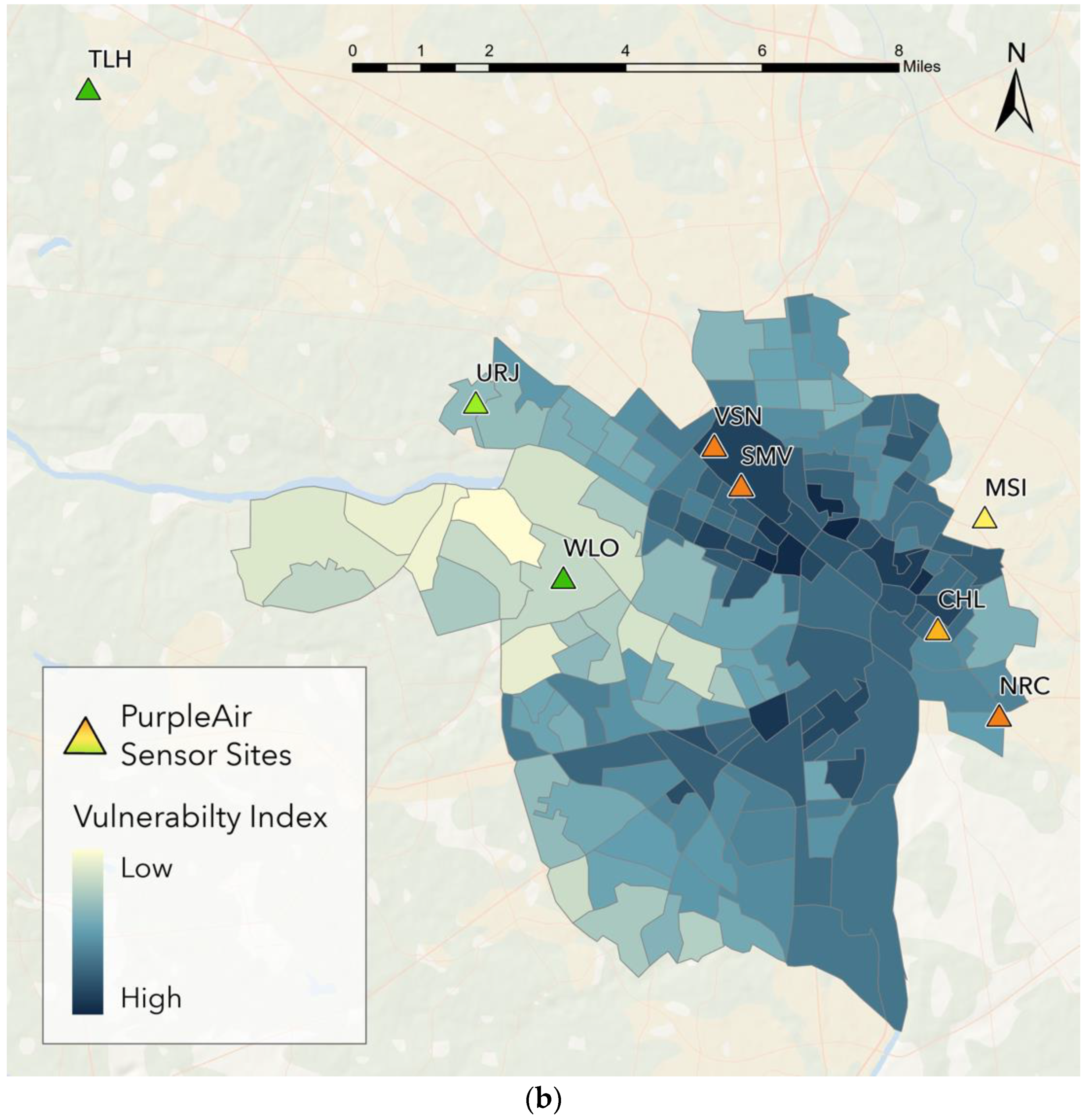
Three sensors were installed in areas of the city that were less likely to experience extreme heat, as indicated by Shandas et al. and the vulnerability index [14]. These are the three westernmost sites in Figure 2, which all fall in more affluent suburban neighborhoods. This is overlaid by census block in Figure 2, with available data within the city limits showing that these sites are more likely to experience socioeconomic and environmental benefits compared to other sites to the east. With this understanding, we aimed to test the null hypothesis that these more affluent neighborhoods do not experience significantly different air quality than their counterparts to the east and more intensely developed parts of the city.

2.3. Analysis of Spatial and Temporal Patterns

Sensors were installed beginning in February 2019, and we analyzed data collected from the sensor network from February 14 to November 14, 2019. Subsequently, all PM2.5 values were run through a corrective equation, using co-temporal temperature (°F) and relative humidity (%) readings, to diminish the degree to which temperature and relative humidity skew PM2.5 measurements in PA-II sensors. The corrective equation used was from a 2020 Environmental Protection Agency report, and the idea of adjusting PM2.5 values based on relative humidity and temperature is also recommended by Zheng et al. (2018) and Malings et al. (2020) [40,41,42].
To assess the reliability of the PA-II measurements, cross-comparisons between two PA-IIs and a Teledyne 640X (T640X) reference instrument were conducted. These sensors were all co-located at the MSI site, next to one another, approximately 2.5 m off of the ground. Including information from both channels (A and B) of the two PA-IIs and from the reference instrument for all available data (10 October 2019–29 October 2020), five total data sets of hourly PM2.5 averages were compared (n = 8976).
The four individual channels (A and B) of the two PA-IIs were all highly correlated (Table 1). Pearson’s correlation analyses yielded R values ranging between 0.97 and 0.99, Spearman’s rank correlations yielded rho values all rounding to 0.99, and linear regression yielded slopes of between 0.97 and 1.04. Similarly, Malings et al. found high self-consistency among nine PA-II units tested [41]. Comparisons between the PA-IIs and the T640X showed moderately strong relationships with correlation coefficients ranging between 0.67 and 0.70, confirming the findings of the aforementioned literature (Table 1). Bulot et al. (2019) and Zheng et al. found similar results among low-cost sensors, with R values from cross-comparisons all ranging from 0.61–0.88 [42,43]. The linear regressions of the comparisons between instrument types yielded slopes ranging from 0.82 to 0.85, indicating a possible bias in the PA-II instruments recording lower PM2.5 values than the T640X.
Because our study was focused specifically on days of extreme heat, we also analyzed the same five data sets (n = 951) for hourly PM2.5 values in which temperature was greater than 90 °F (32.2 °C). The four individual channels of the two PA-IIs were again highly correlated by all measures (Table 2). Comparisons between the PA-IIs and the T640X showed moderately strong relationships marginally weaker than the previous analysis. Given the extremely high inter-channel and inter-sensor reliability between the PA-II sensors, this confirms that the PA-II is relatively reliable for detecting large-scale trends among the different PA-II locations (as is the scope of this research), but the instruments are not highly precise for monitoring of absolute values in comparison to the TS60X instrument.
Because previous studies have implicated both extreme temperatures and poor air quality as adverse environmental conditions that disproportionately harm marginalized communities, comparing the mean temperature and PM2.5 concentrations on the ten hottest days of 2019 allowed us to test this relationship [5,11,15]. These days were selected based on a combination of temperature data from the NOAA weather station at Richmond International Airport and readings from the PurpleAir sensors themselves. To assess overall correlations between temperature and PM2.5, we compared the daily temperature and PM2.5 averages using the entire record of available data. For all other analyses, data from the ten hottest days were used.
We first compared the temperature between the eight sample locations. This project follows from a previous study that measured the urban heat island effect (UHI) in Richmond. Shandas et al. combined satellite and ground temperature measurements to map UHI throughout different times of day [14]. From these earlier data, we were able to predict which sensors were located in hotter versus cooler areas of the city. We used these predictions to help determine locations for the sensors as part of the sample design, and we validated the temperature predictions with the sensor data using an analysis of variance (ANOVA) test and the post hoc Tukey’s range test. These analyses were conducted in R version 1.2.1335 and included the eight sensors aggregated by hourly average temperature distributions for the ten hottest days. Differences in temperature among the sensors were highlighted at the 95% confidence level. These findings were remapped onto the city landscape to visualize the spatial patterns.
We next evaluated the relationship between daily average temperature and PM2.5 values using a Pearson’s correlation analysis with the entire 2019 data set. Daily averages of PM2.5 and temperature on the ten hottest days at individual sites were also compared using a single sample t-test (α < 0.05). To assess diurnal patterns of air pollution during the ten hottest days, we plotted the average hourly PM2.5 values of each sensor at each hour of the day to determine how PM2.5 fluctuated during these days. Finally, PM2.5 values from each sensor were analyzed using an analysis of variance (ANOVA) test and post hoc Tukey’s range test. Readings were aggregated by hourly average PM2.5 distributions for the ten hottest days. Differences in PM2.5 among the sensors were highlighted at the 95% confidence level. These findings were remapped onto the city landscape to visualize the spatial patterns.

3. Results

3.1. Spatial Variability in Urban Temperatures

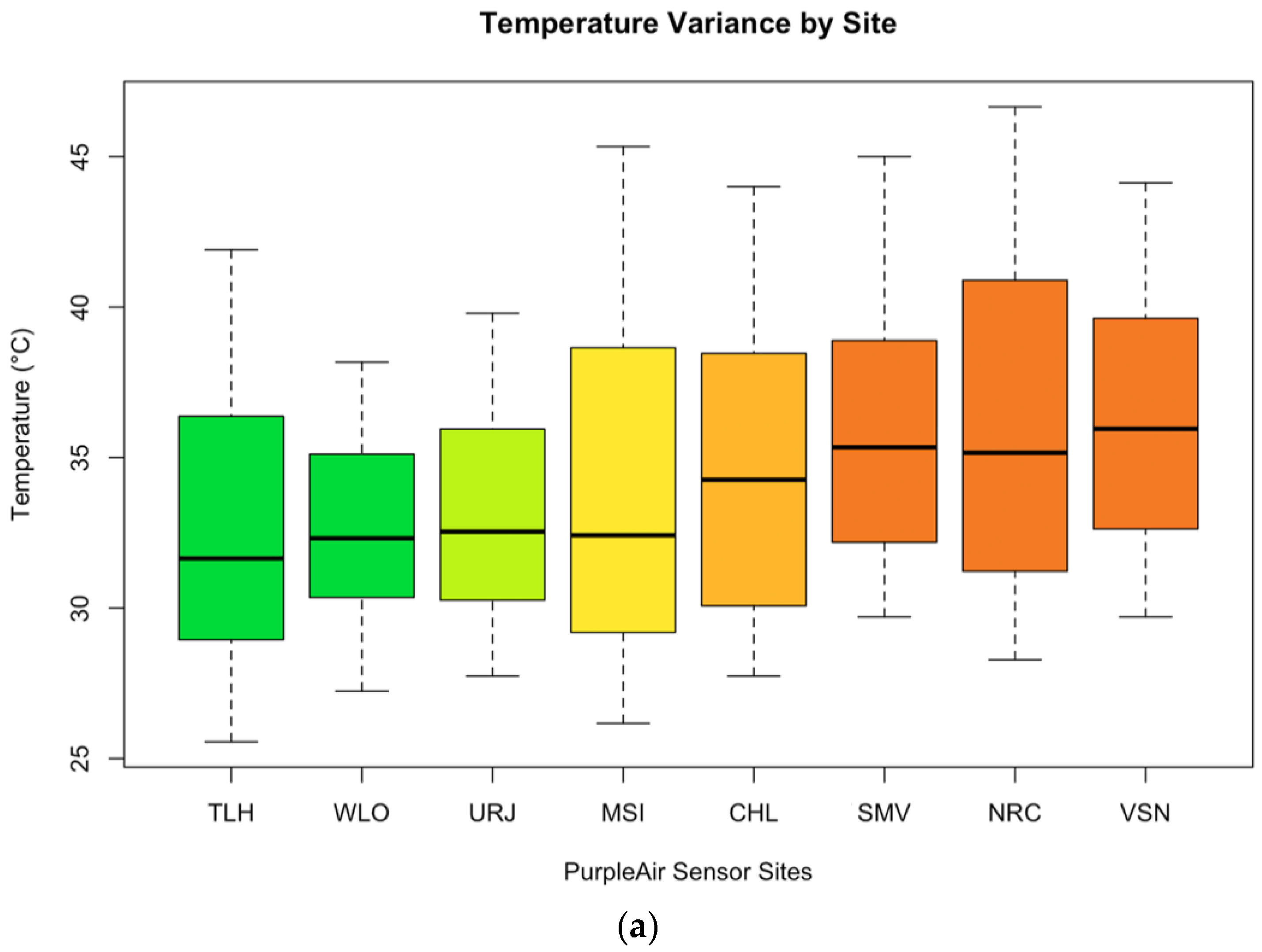
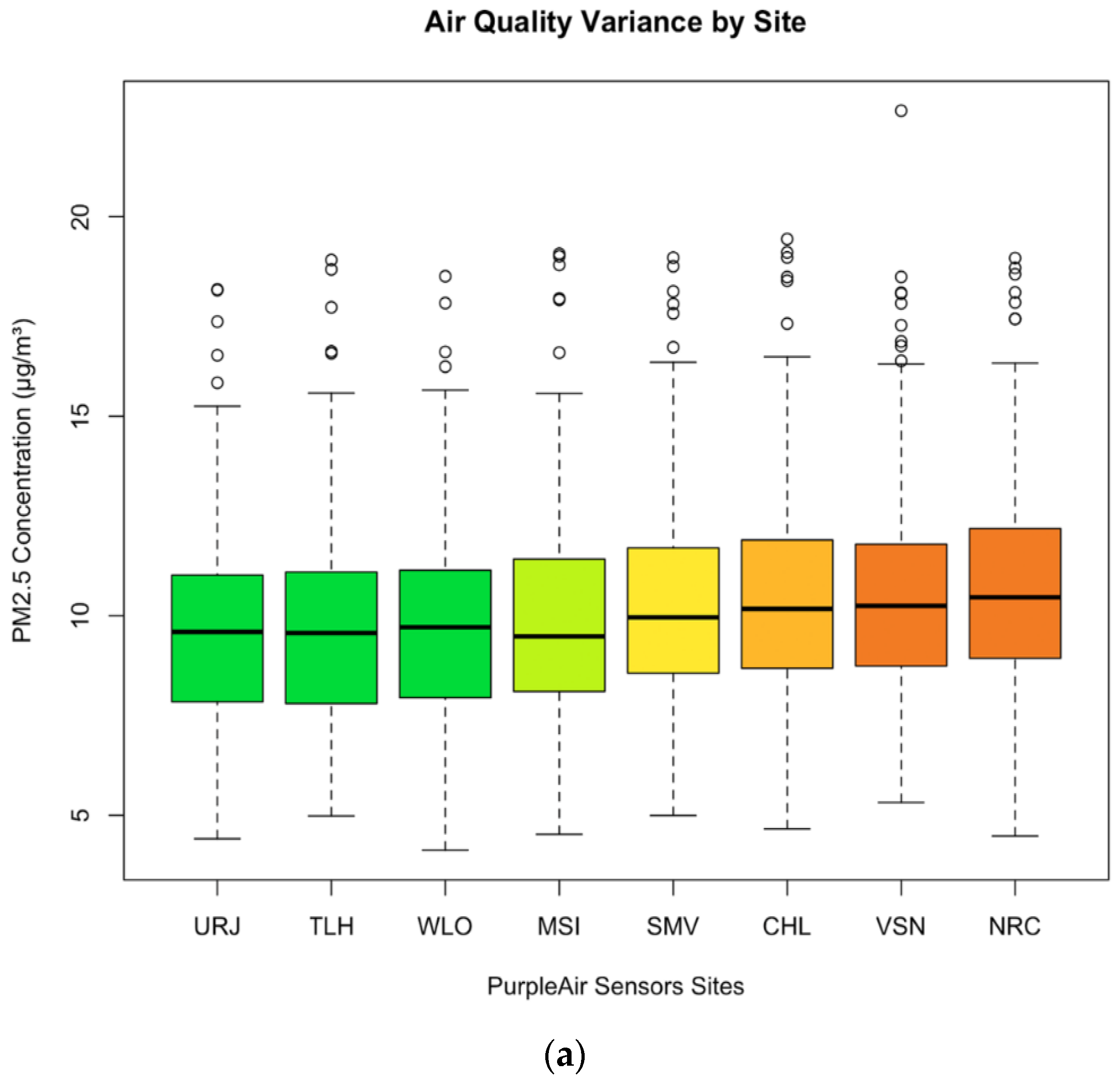
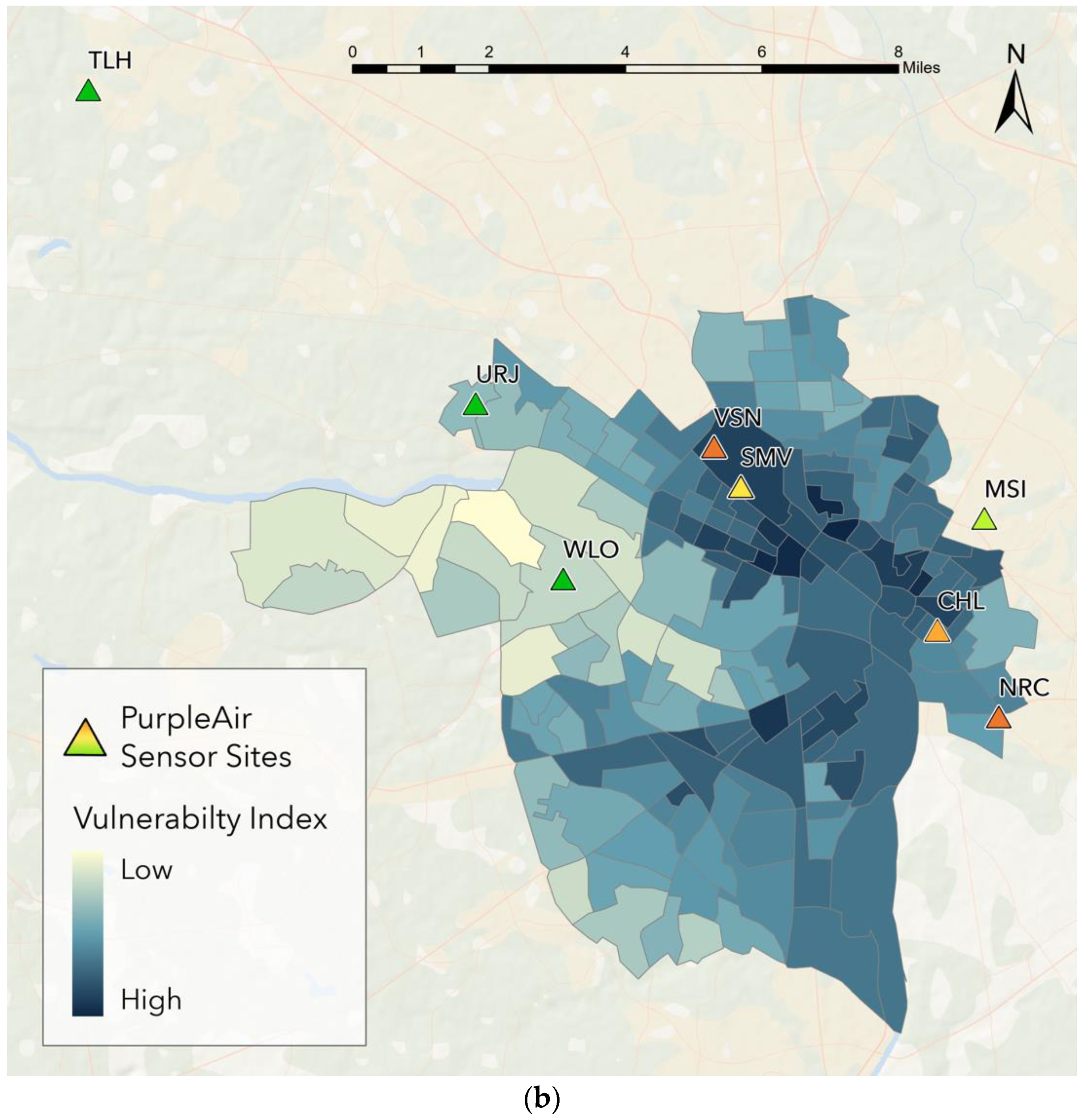
Using the temperature readings from the PurpleAir sensors, the UHI patterns from the earlier Shandas et al. study were confirmed [14]. An analysis of variance (ANOVA) on hourly temperature averages for each sensor on the ten hottest days of 2019 yielded highly significant variation among sites (F(7, 1768) = 29.47; p < 0.001). A post hoc Tukey’s range test identified five distinct groups that differed significantly from each other at p < 0.05 (Figure 3a). In accordance with initial predictions, communities in the west end of the city were indeed the coolest, falling in the two lowest temperature categories out of the five. This pattern is represented spatially in Figure 3b, overlaid with the same vulnerability index as Figure 2. While there was variation in the overall east-west pattern, the temperature of the sites generally mirrored spatial trends of vulnerability and development intensity through the city, as well as the findings of Shandas et al. [14].

3.2. Connections between Urban Temperatures and Air Quality

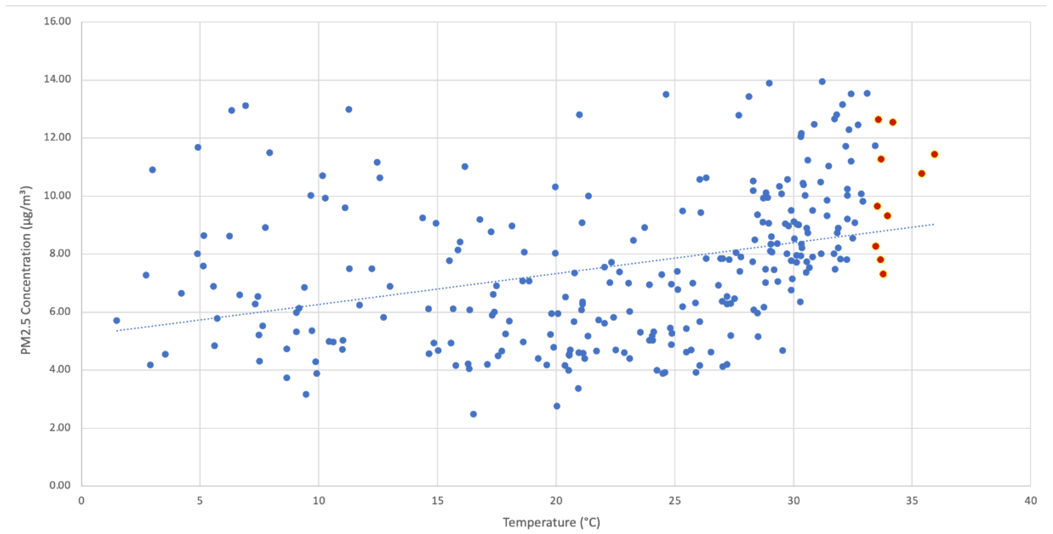
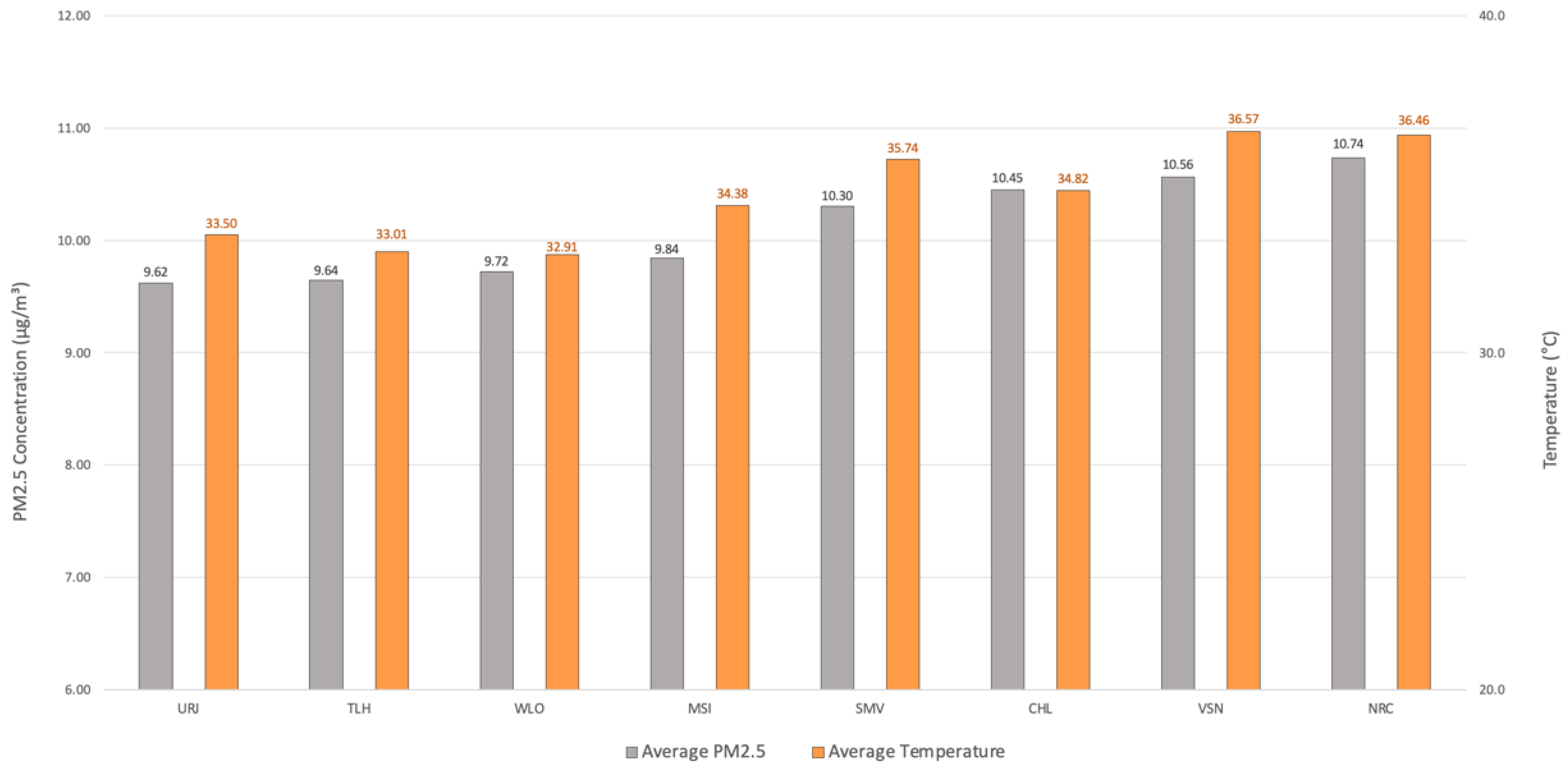
Combining all available data from February 14 to November 14, the daily temperature averaged across all sensors exhibited a weak positive correlation with daily PM2.5 values (R = 0.35). There was a distinct cluster of consistently high PM2.5 values on the hottest days, with much higher scatter signifying little to no correlation on cooler days (Figure 4). To unpack this relationship, we extracted the average temperature and PM2.5 values from each sensor over the ten hottest days of 2019 (Figure 5). Overall, the mean PM2.5 values were significantly higher (t(9) = 3.89; p < 0.01) on the ten hottest days (10.10 μg/m3) than for the total 2019 record (7.60 μg/m3). This supports the conclusion that hot summer days warranted the greatest concern with regard to understanding which parts of the city were experiencing the highest levels of air pollution.

3.3. Diurnal Patterns in Urban Air Quality

The sensors exhibited a relatively consistent diurnal pattern in hourly PM2.5 values for the ten hottest days of the year. PM2.5 peaked in the early morning when relative humidity was also at its highest, reaching its minimum in the early afternoon, and consistently rose throughout the late afternoon and into the evening (Figure 6). All sensors displayed a common cyclicity, with the exception of the VSN sensor, which showed pronounced spikes around the morning and evening rush hour periods. The most likely explanation for this anomaly is the industrialized area where the VSN sensor is located, as well as the heavy traffic the area experiences. Otherwise, the rank order of best to worst air quality remained relatively consistent among sensors throughout the day, which begins to demonstrate the spatial variability between sites.

3.4. Spatial Patterns in Urban Air Quality

The mean hourly PM2.5 measurements were significantly different among the eight sensors analyzed for the ten hottest days of 2019 (F(7, 1899) = 2.24; p < 0.001). A Tukey’s test sorted the eight sites into five groups of significant difference at p < 0.05 (Figure 7a). Although the variance among sites was less pronounced than the variability in temperature given the lower F-value, a geographic representation of the distribution of air quality confirmed the general pattern of Richmond’s west end enjoying greater environmental amenities than the east end (Figure 7b).
The spatial patterns of PM2.5 air pollution were generally consistent with those previously described for temperature, though slightly less pronounced. The top two rank-ordered sites (NRC and VSN) and bottom three sites (URJ, TLH, and WLO) were the same between the temperature and PM2.5 Tukey’s tests. Furthermore, the three westernmost sites were the lowest in both categories, illustrating the disparity in environmental outcomes for residents of the city of Richmond.

4. Discussion

Statistically significant differences were observed for both temperature and PM2.5 among the eight sensors, with temperature displaying greater variability. Five significantly different temperature groups were recorded, while three groups were identified among PM2.5 values. In general, sites with lower PM2.5 also yielded lower temperatures, which followed a geographic pattern as well. Sites in the west end (URJ, TLH, and WLO) consistently yielded lower temperatures and PM2.5 values. Sites in the east end (NRC, MSI, and CHL) and those closer to the urban core (VSN and SMV) had higher PM2.5 and temperature readings, and the temperature-PM2.5 relationship was closely correlated but did not match exactly. These findings suggest the existence of a west–east trend, but it appears to level off east of the urban core, with the more vulnerable and lower-income communities in the east end experiencing poor environmental quality similar to the more intensely developed parts of the city. Conversely, the wealthier communities in the west end generally enjoy greater environmental amenities, including better air quality and fewer instances of extreme heat. These improved environmental conditions, combined with fewer socioeconomic- and health-related stressors, have been found to result in life expectancies of up to twenty years higher in these neighborhoods compared to their more vulnerable counterparts [44].
It should be noted, however, that despite the high inter-sensor correlation exhibited among sample PA-IIs (as shown in Section 2.3), it cannot be ruled out that disparities between PM2.5 readings among the eight sensors analyzed could be explained in part due to random chance. While Malings et al. found the mean absolute error of PA-II units for short-term measurements to be of similar magnitude to some of the differences among sites observed in our study, they reported long-term annual errors to be less than 1 μg/m3. This finding suggests continued monitoring of these sites. To mitigate uncertainty surrounding potential inter-sensor variability in continued and/or replicating research with low-cost sensors, calibration via inter-sensor validation and normalization with a reference instrument before sensor deployment are encouraged to provide an additional layer of confidence in the accuracy of readings [41].
These findings are consistent with the results of previous studies examining the spatial variability of temperature in cities. Voelkel et al. (2018) and Vargo et al. (2016) similarly found spatial variability in the severity of the urban heat island (UHI) effect, as well as disproportionate impacts on socioeconomically vulnerable communities. Shandas et al. also found a highly variable intra-urban spatial distribution of extreme temperatures in three cities, including Richmond [14]. Analyses at a higher resolution and greater extent would be required to draw more robust conclusions regarding the causes and effects of UHI in Richmond and other cities. Still, there is a clear central tendency of inequality among societal and ecological impacts presented by UHI in cities, and effective mitigation through more innovative urban design and land use planning techniques is required to combat this. These solutions include wider accessibility of urban parks and vegetation, as well as greater prevalence and heterogeneity of permeable and high albedo surfaces such as green roofs and light-colored asphalt [12,23,45].
Importantly, we found that these spatial patterns of extreme heat were associated with similar, slightly weaker differences in air quality. Sadd et al. (2011) and Mikati et al. (2018) have previously noted spatial variability in the distribution of particulate matter and other pollutants in urban settings. Others have found that particulate matter and greenhouse gas emissions exacerbate UHI, drawing a causal connection between temperature and air quality [11,15]. Additionally, numerous studies have found that socioeconomically disenfranchised communities experience disproportionate impacts from both the causes and effects of poor air quality [6,8,9]. Our findings support a general trend of worsening air quality from the more affluent, white communities in the west towards the urban core and eastern part of the city, although higher, neighborhood-level resolution sampling would be required to substantiate more specific demographic patterns.
Despite their apparent interaction, few prior studies have attempted to tie together air quality, extreme heat, and socioeconomic vulnerability. Leong et al. (2018) and Grove et al. (2018), for example, identified both extreme heat and poor air quality as environmental stressors (or “disamenities”) to which socioeconomically vulnerable communities are exposed, but the physical relationship between temperature and air quality was not their focus. To this end, policy decisions and remediation actions rarely take into account the correlational and causal relationships between UHI and air pollution, as well as their disproportionate impacts on vulnerable communities. For example, many proposed responses to UHI, such as the creation of more urban parks and increasing vegetation cover, can serve to mitigate poor air quality as an additional benefit [24,25]. Furthermore, reducing reliance on fossil fuels, moving fossil fuel and other industrial facilities (when they cannot be removed or decommissioned) away from vulnerable communities, and implementing more efficient transportation infrastructure can result in decreased emissions and help solve many of these issues at their root [8,10,29]. This more holistic perspective has never been more important. As has been learned from studies during the COVID-19 pandemic, reducing exposure to particulate matter for at-risk populations by even a small amount could substantially reduce susceptibility to respiratory diseases and prevent unnecessary deaths, especially among racial and ethnic minorities, who have been disproportionately impacted by the disease [4,46].
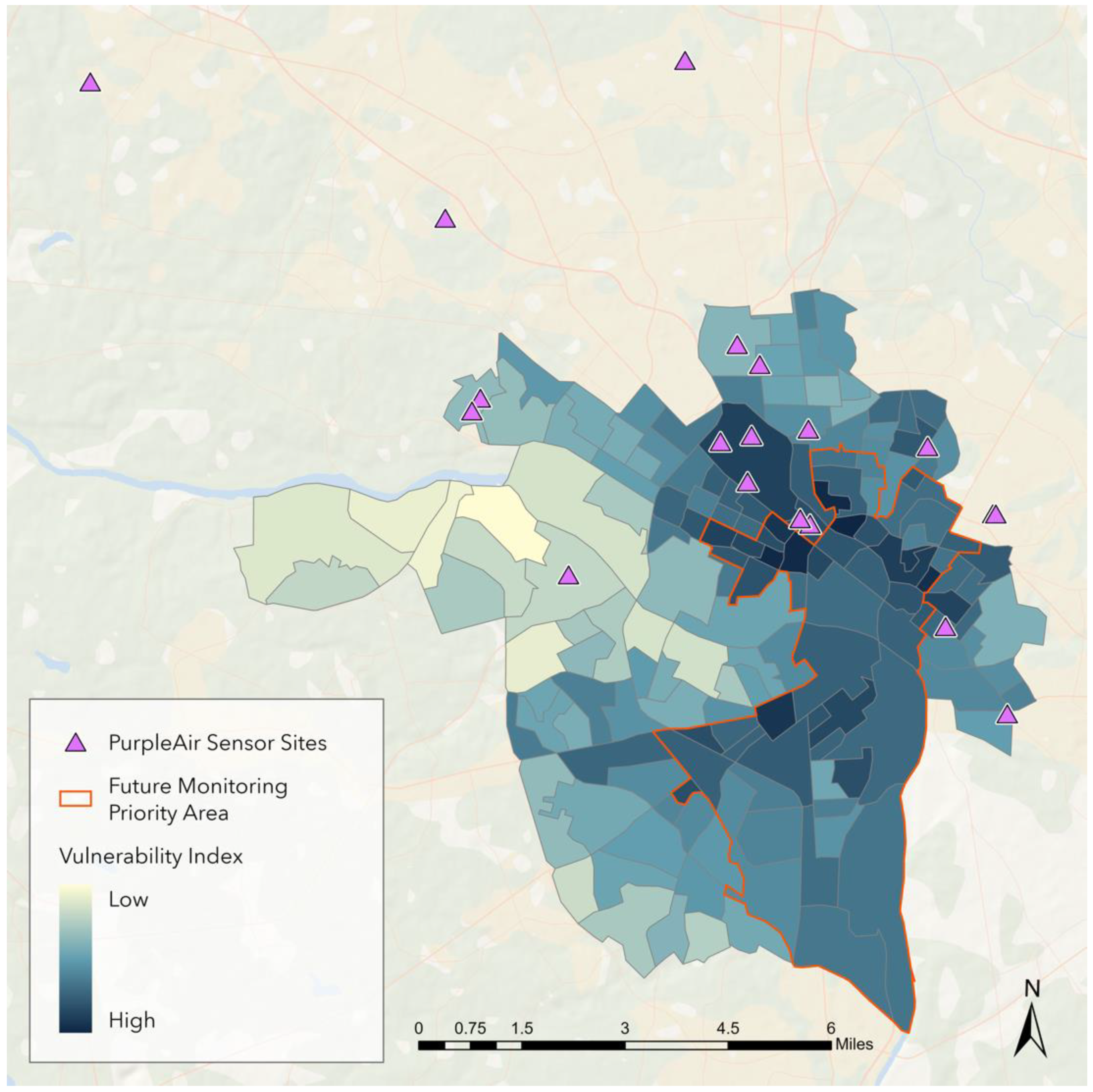
Future studies would also benefit from greater coverage and a higher spatial resolution network of sensors. In accordance with our understanding of how large emitters and vulnerable communities are spatially distributed throughout the city (Figure 1a and Figure 2), there are areas in need of monitoring that have not been reached. Relatively inexpensive sensors such as the PurpleAir PA-II provide the opportunity to expand the network economically, and plans are already in place through community partnerships to increase the number of stationary sensors in the region to 30–40 in total. However, important gaps remain in the network. Specifically, downtown and the south side of Richmond are the highest priority, as the south side has a significant industrial presence, and they both have heavy vehicle traffic and relatively high vulnerability (Figure 8). Future monitoring should ensure that predicted areas of high vulnerability to poor air quality are represented in sampling.
Given the rough spatial granularity provided by stationary sensors, mobile sensing can be employed as a supplement. Stationary sensors are advantageous in that they report a consistent stream of data from a single location, which provides high temporal resolution, allows temporal trends to be accurately measured, and with a broad enough network of monitoring sites, can outline a rough spatial model of air quality. Conversely, mobile air quality sensors can be employed in short sessions over long transects, gathering high-resolution spatial data within a small window of time (in which monitoring conditions are minimally variable). Mobile sensing campaigns can be most optimally carried out with a large group of individuals, each traveling along pre-assigned transects within the sampling area over approximately an hour. These efforts can then be repeated over numerous sampling sessions during different times of day and seasons of the year, measuring air quality over large areas with high spatial resolution and accounting for a wide range of conditions. With proper redundancy, mobile sensing can provide a high spatial resolution representation of air quality to fill in the gaps left by stationary monitoring. When combined, stationary and mobile monitoring could be used to track the spatial and temporal variability in air quality relevant to socioeconomic and health vulnerability.
In addition, detecting a wider range of pollutants would enhance the accuracy of modeling air quality on a city-wide scale. Reliable PM2.5 monitoring equipment is relatively cheap and accessible compared to that of other pollutants, and PM2.5 is a fairly accurate proxy for overall air quality. However, it is merely one pollutant among numerous other gases and aerosols that are heavily emitted and thus cannot holistically represent the spatial representation of air pollution [38,47]. Investing in more expensive equipment and more robust sampling of pollutants such as CO, CO2, NO2, O3, and SO2 would provide a more comprehensive and precise representation of air quality and its potential impacts. Closer tracking of humidity would also be valuable to garner a complete overall picture. For example, certain components of the diurnal cycle of PM2.5 observed in our study could be attributed to the fact that high relative humidity can slightly skew the PurpleAir’s PM2.5 readings, which would result in inflated values in the morning when relative humidity is at its highest [48,49]. While this was partially mitigated using the EPA’s corrective equation, it does demonstrate a limitation of these devices.
More long-term data are needed to substantiate connections between inequitable distributions of air quality and socioeconomic, health, and geographic factors. Still, the results of this study begin to illustrate the contributions of various land-use factors that correlate with poor air quality and the socioeconomic outcomes and urban environmental justice issues to which they are tied. These impacts have not been addressed throughout the history of Richmond and many cities like it, and such blind spots must be acknowledged and systematically removed. Given this understanding, awareness of these issues can impact policy and decision-making on local and regional scales, resulting in the mitigation of poor air quality and extreme heat at their source and helping to tackle the environmental inequalities that have plagued vulnerable communities for decades.

Author Contributions

Conceptualization, A.M.E., T.R.L., J.S.H., and S.S.F.; methodology, A.M.E., T.R.L., and J.S.H.; software, A.M.E.; validation, A.M.E., T.R.L., J.S.H., and S.S.F.; formal analysis, A.M.E.; investigation, A.M.E., T.R.L., J.S.H., K.C.S., and S.S.F.; resources, T.R.L., J.S.H., and S.S.F.; data curation, A.M.E.; writing—original draft preparation, A.M.E., T.R.L.; writing—review and editing, A.M.E., T.R.L., J.S.H., K.C.S., and S.S.F.; visualization, A.M.E.; supervision, T.R.L. and J.S.H.; project administration, A.M.E., T.R.L., and J.S.H.; funding acquisition, A.M.E., T.R.L., J.S.H, and S.S.F. All authors have read and agreed to the published version of the manuscript.

Funding

This study received funding for equipment from the School of Arts and Sciences and the Department of Geography and the Environment at the University of Richmond, as well as support from the Virginia Commonwealth University Community Engagement grant program. Funding for this project and ongoing research was also provided to the Science of Museum of Virginia through a grant from the Institute of Museum and Library Services (FAIN #MA-20-19-0255-19).

Acknowledgments

The authors would like to thank the community members who hosted sensors, including Justin Doyle, Chris Burnside, Karl Green, Väsen Brewing Company, the Neighborhood Resource Center of Greater Fulton, and the MathScience Innovation Center. We would also like to thank Namita Verma of the Virginia Department of Environmental Quality for providing DEQ reference instrument PM2.5 data. J.S.H. acknowledges support from the Institute of Museum and Library Services under grant #MA-20-19-0255-19. The views, findings, conclusions or recommendations expressed in this article do not necessarily represent those of the Institute of Museum and Library Services.

Conflicts of Interest

The authors declare no conflict of interest. The funders had no role in the design of the study; in the collection, analyses, or interpretation of data; in the writing of the manuscript, or in the decision to publish the results.

References

  1. Bowatte, G.; Lodge, C.; Lowe, A.J.; Erbas, B.; Perret, J.; Abramson, M.J.; Matheson, M.; Dharmage, S.C. The influence of childhood traffic-related air pollution exposure on asthma, allergy and sensitization: A systematic review and a meta-analysis of birth cohort studies. Allergy 2015, 70, 245–256. [Google Scholar] [CrossRef]
  2. Gehring, U.; Wijga, A.H.; Brauer, M.; Fischer, P.; De Jongste, J.C.; Kerkhof, M.; Oldenwening, M.; Smit, H.A.; Brunekreef, B. Traffic-related Air Pollution and the Development of Asthma and Allergies during the First 8 Years of Life. Am. J. Respir. Crit. Care Med. 2010, 181, 596–603. [Google Scholar] [CrossRef] [Green Version]
  3. Dockery, D.W.; Pope, C.A.; Xu, X.; Spengler, J.D.; Ware, J.H.; Fay, M.E.; Ferris, B.G.; Speizer, F.E. An Association between Air Pollution and Mortality in Six U.S. Cities. N. Engl. J. Med. 1993, 329, 1753–1759. [Google Scholar] [CrossRef] [Green Version]
  4. Wu, X.; Nethery, R.C.; Sabath, B.M.; Braun, D.; Dominici, F. Air pollution and COVID-19 mortality in the United States: Strengths and limitations of an ecological regression analysis. Sci. Adv. 2020, 6, eabd4049. [Google Scholar] [CrossRef]
  5. Grove, M.; Ogden, L.; Pickett, S.; Boone, C.; Buckley, G.; Locke, D.H.; Lord, C.; Hall, B. The Legacy Effect: Understanding How Segregation and Environmental Injustice Unfold over Time in Baltimore. Ann. Am. Assoc. Geogr. 2018, 108, 524–537. [Google Scholar] [CrossRef]
  6. Mohai, P.; Lantz, P.M.; Morenoff, J.; House, J.S.; Mero, R.P. Racial and Socioeconomic Disparities in Residential Proximity to Polluting Industrial Facilities: Evidence From the Americans’ Changing Lives Study. Am. J. Public Health 2009, 99, S649–S656. [Google Scholar] [CrossRef]
  7. Mikati, I.; Benson, A.F.; Luben, T.J.; Sacks, J.D.; Richmond-Bryant, J. Disparities in Distribution of Particulate Matter Emission Sources by Race and Poverty Status. Am. J. Public Health 2018, 108, 480–485. [Google Scholar] [CrossRef]
  8. Fumes across the Fence-Line: The Health Impacts of Air Pollution from Oil & Gas Facilities on African American Communities. NAACP & CATF. 2017. Available online: https://bit.ly/2K632jW (accessed on 12 May 2020).
  9. King, K.E. Chicago residents’ perceptions of air quality: Objective pollution, the built environment, and neighborhood stigma theory. Popul. Environ. 2015, 37, 1–21. [Google Scholar] [CrossRef] [Green Version]
  10. Finley-Brook, M.; Williams, T.L.; Caron-Sheppard, J.A.; Jaromin, M.K. Critical energy justice in US natural gas infrastructuring. Energy Res. Soc. Sci. 2018, 41, 176–190. [Google Scholar] [CrossRef]
  11. Sachindra, D.A.; Ng, A.; Muthukumaran, S.; Perera, B.J.C. Impact of climate change on urban heat island effect and extreme temperatures: A case-study. Q. J. R. Meteorol. Soc. 2015, 142, 172–186. [Google Scholar] [CrossRef]
  12. Connors, J.P.; Galletti, C.S.; Chow, W.T.L. Landscape configuration and urban heat island effects: Assessing the relationship between landscape characteristics and land surface temperature in Phoenix, Arizona. Landsc. Ecol. 2013, 28, 271–283. [Google Scholar] [CrossRef]
  13. Vargo, J.; Stone, B.; Habeeb, D.; Liu, P.; Russell, A. The social and spatial distribution of temperature-related health impacts from urban heat island reduction policies. Environ. Sci. Policy 2016, 66, 366–374. [Google Scholar] [CrossRef]
  14. Shandas, V.; Voelkel, J.; Williams, J.; Hoffman, J. Integrating Satellite and Ground Measurements for Predicting Locations of Extreme Urban Heat. Climate 2019, 7, 5. [Google Scholar] [CrossRef] [Green Version]
  15. Tan, J.; Zheng, Y.; Tang, X.; Guo, C.; Li, L.; Song, G.; Zhen, X.; Yuan, D.; Kalkstein, A.J.; Li, F.; et al. The urban heat island and its impact on heat waves and human health in Shanghai. Int. J. Biometeorol. 2010, 54, 75–84. [Google Scholar] [CrossRef]
  16. Voelkel, J.; Hellman, D.; Sakuma, R.; Shandas, V. Assessing Vulnerability to Urban Heat: A Study of Disproportionate Heat Exposure and Access to Refuge by Socio-Demographic Status in Portland, Oregon. Int. J. Environ. Res. Public Health 2018, 15, 640. [Google Scholar] [CrossRef] [Green Version]
  17. Alonso, L.; Renard, F. A Comparative Study of the Physiological and Socio-Economic Vulnerabilities to Heat Waves of the Population of the Metropolis of Lyon (France) in a Climate Change Context. Int. J. Environ. Res. Public Health 2020, 17, 1004. [Google Scholar] [CrossRef] [Green Version]
  18. Willow, A.J. The new politics of environmental degradation: Un/expected landscapes of disempowerment and vulnerability. J. Polit. Ecol. 2014, 21, 237–257. [Google Scholar] [CrossRef] [Green Version]
  19. Leong, M.; Dunn, R.R.; Trautwein, M.D. Biodiversity and socioeconomics in the city: A review of the luxury effect. Biol. Lett. 2018, 14, 20180082. [Google Scholar] [CrossRef]
  20. Twohig-Bennett, C.; Jones, A. The health benefits of the great outdoors: A systematic review and meta-analysis of greenspace exposure and health outcomes. Environ. Res. 2018, 166, 628–637. [Google Scholar] [CrossRef]
  21. Choi, D.-A.; Park, K.; Rigolon, A. From XS to XL Urban Nature: Examining Access to Different Types of Green Space Using a ‘Just Sustainabilities’ Framework. Sustainability 2020, 12, 6998. [Google Scholar] [CrossRef]
  22. Meili, N.; Manoli, G.; Burlando, P.; Bou-Zeid, E.; Chow, W.T.L.; Coutts, A.M.; Daly, E.; Nice, K.A.; Roth, M.; Tapper, N.J.; et al. An urban ecohydrological model to quantify the effect of vegetation on urban climate and hydrology (UT&C v1.0). Geosci. Model Dev. 2020, 13, 335–362. [Google Scholar] [CrossRef] [Green Version]
  23. Nuruzzaman Urban Heat Island: Causes, Effects and Mitigation Measures—A Review. Int. J. Environ. Monit. Anal. 2015, 3, 67. [CrossRef] [Green Version]
  24. Irga, P.; Burchett, M.; Torpy, F.R. Does urban forestry have a quantitative effect on ambient air quality in an urban environment? Atmos. Environ. 2015, 120, 173–181. [Google Scholar] [CrossRef] [Green Version]
  25. Baraldi, R.; Chieco, C.; Neri, L.; Facini, O.; Rapparini, F.; Morrone, L.; Rotondi, A.; Carriero, G. An integrated study on air mitigation potential of urban vegetation: From a multi-trait approach to modeling. Urban For. Urban Green. 2019, 41, 127–138. [Google Scholar] [CrossRef]
  26. Misra, P.; Imasu, R.; Takeuchi, W. Impact of Urban Growth on Air Quality in Indian Cities Using Hierarchical Bayesian Approach. Atmosphere 2019, 10, 517. [Google Scholar] [CrossRef] [Green Version]
  27. Wang, L.; Zhang, H.; Mao, L.; Li, S.; Wu, H. Assessing Spatiotemporal Characteristics of Urban PM2.5 Using Fractal Dimensions and Wavelet Analysis. Math. Probl. Eng. 2020, 2020, 1–15. [Google Scholar] [CrossRef]
  28. Mead, M.; Popoola, O.; Stewart, G.; Landshoff, P.V.; Calleja, M.; Hayes, M.J.; Baldovi, J.; McLeod, M.; Hodgson, T.; Dicks, J.; et al. The use of electrochemical sensors for monitoring urban air quality in low-cost, high-density networks. Atmos. Environ. 2013, 70, 186–203. [Google Scholar] [CrossRef] [Green Version]
  29. Sadd, J.L.; Pastor, M.; Morello-Frosch, R.; Scoggins, J.; Jesdale, B.M. Playing It Safe: Assessing Cumulative Impact and Social Vulnerability through an Environmental Justice Screening Method in the South Coast Air Basin, California. Int. J. Environ. Res. Public Health 2011, 8, 1441–1459. [Google Scholar] [CrossRef]
  30. The Racial Dot Map. Racial Demographics Group, University of Virginia. 2013. Available online: https://bit.ly/34PkyT3 (accessed on 21 May 2020).
  31. Quickfacts: Richmond City, Virginia. U.S. Census Bureau. 2019. Available online: https://bit.ly/2Hywh03 (accessed on 22 November 2019).
  32. Asthma Capitals: The Most Challenging Places to Live With Asthma. Asthma and Allergy Foundation of America. 2018. Available online: https://bit.ly/2FqZcBm (accessed on 19 June 2019).
  33. Virginia: State Profile and Energy Estimates. U.S. Energy Information Administration. 2017. Available online: https://bit.ly/2QgCiCJ (accessed on 30 May 2019).
  34. RVAgreen Sustainability Dashboard. City of Richmond RVAgreen 2050, N.D. Available online: https://bit.ly/3asWYfL (accessed on 3 July 2020).
  35. PurpleAir PA-II—Summary Report. South Coast Air Quality Management District. 2017. Available online: https://bit.ly/3k5W6n3 (accessed on 7 June 2019).
  36. Kelly, F.J.; Fussell, J.C. Size, source and chemical composition as determinants of toxicity attributable to ambient particulate matter. Atmos. Environ. 2012, 60, 504–526. [Google Scholar] [CrossRef]
  37. Kim, K.-H.; Kabir, E.; Kabir, S. A review on the human health impact of airborne particulate matter. Environ. Int. 2015, 74, 136–143. [Google Scholar] [CrossRef]
  38. Engel-Cox, J.A.; Oanh, N.T.K.; Van Donkelaar, A.; Martin, R.V.; Zell, E. Toward the next generation of air quality monitoring: Particulate Matter. Atmos. Environ. 2013, 80, 584–590. [Google Scholar] [CrossRef]
  39. Extreme Heat & Public Health. City of Richmond RVAgreen 2050, N.D. Available online: https://bit.ly/30s8N4l (accessed on 28 July 2020).
  40. Barkjohn, K.; Gantt, B.; VonWald, I.; Clements, A. PurpleAir PM2.5 Performance across the U.S. United States Environmental Protection Agency. 2020. Available online: https://bit.ly/3duEz5w (accessed on 3 October 2020).
  41. Malings, C.; Tanzer, R.; Hauryliuk, A.; Saha, P.K.; Robinson, A.L.; Presto, A.A.; Subramanian, R. Fine particle mass monitoring with low-cost sensors: Corrections and long-term performance evaluation. Aerosol Sci. Technol. 2020, 54, 160–174. [Google Scholar] [CrossRef]
  42. Zheng, T.; Bergin, M.H.; Johnson, K.K.; Tripathi, S.N.; Shirodkar, S.; Landis, M.; Sutaria, R.; Carlson, D.E. Field evaluation of low-cost particulate matter sensors in high- and low-concentration environments. Atmos. Meas. Tech. 2018, 11, 4823–4846. [Google Scholar] [CrossRef] [Green Version]
  43. Bulot, F.M.J.; Johnston, S.J.; Basford, P.J.; Easton, N.H.C.; Apetroaie-Cristea, M.; Foster, G.L.; Morris, A.K.R.; Cox, S.J.; Loxham, M. Long-term field comparison of multiple low-cost particulate matter sensors in an outdoor urban environment. Sci. Rep. 2019, 9, 1–13. [Google Scholar] [CrossRef] [PubMed]
  44. 20 Years in Richmond, Virginia. Virginia Commonwealth University Center on Society and Health. 12 November 2015. Available online: https://bit.ly/33vdhZN (accessed on 4 August 2020).
  45. Price, A.; Jones, E.C.; Jefferson, F. Vertical Greenery Systems as a Strategy in Urban Heat Island Mitigation. Water Air Soil Pollut. 2015, 226, 1–11. [Google Scholar] [CrossRef]
  46. Schulz, A.J.; Mehdipanah, R.; Chatters, L.M.; Reyes, A.G.; Neblett, J.E.W.; Israel, B.A. Moving Health Education and Behavior Upstream: Lessons From COVID-19 for Addressing Structural Drivers of Health Inequities. Health Educ. Behav. 2020, 47, 519–524. [Google Scholar] [CrossRef]
  47. Castell, N.; Dauge, F.R.; Schneider, P.; Vogt, M.; Lerner, U.; Fishbain, B.; Broday, D.; Bartonova, A. Can commercial low-cost sensor platforms contribute to air quality monitoring and exposure estimates? Environ. Int. 2017, 99, 293–302. [Google Scholar] [CrossRef]
  48. Ephrath, J.; Goudriaan, J.; Marani, A. Modelling diurnal patterns of air temperature, radiation wind speed and relative humidity by equations from daily characteristics. Agric. Syst. 1996, 51, 377–393. [Google Scholar] [CrossRef]
  49. Jayaratne, R.; Liu, X.; Thai, P.; Dunbabin, M.; Morawska, L. The influence of humidity on the performance of a low-cost air particle mass sensor and the effect of atmospheric fog. Atmos. Meas. Tech. 2018, 11, 4883–4890. [Google Scholar] [CrossRef] [Green Version]
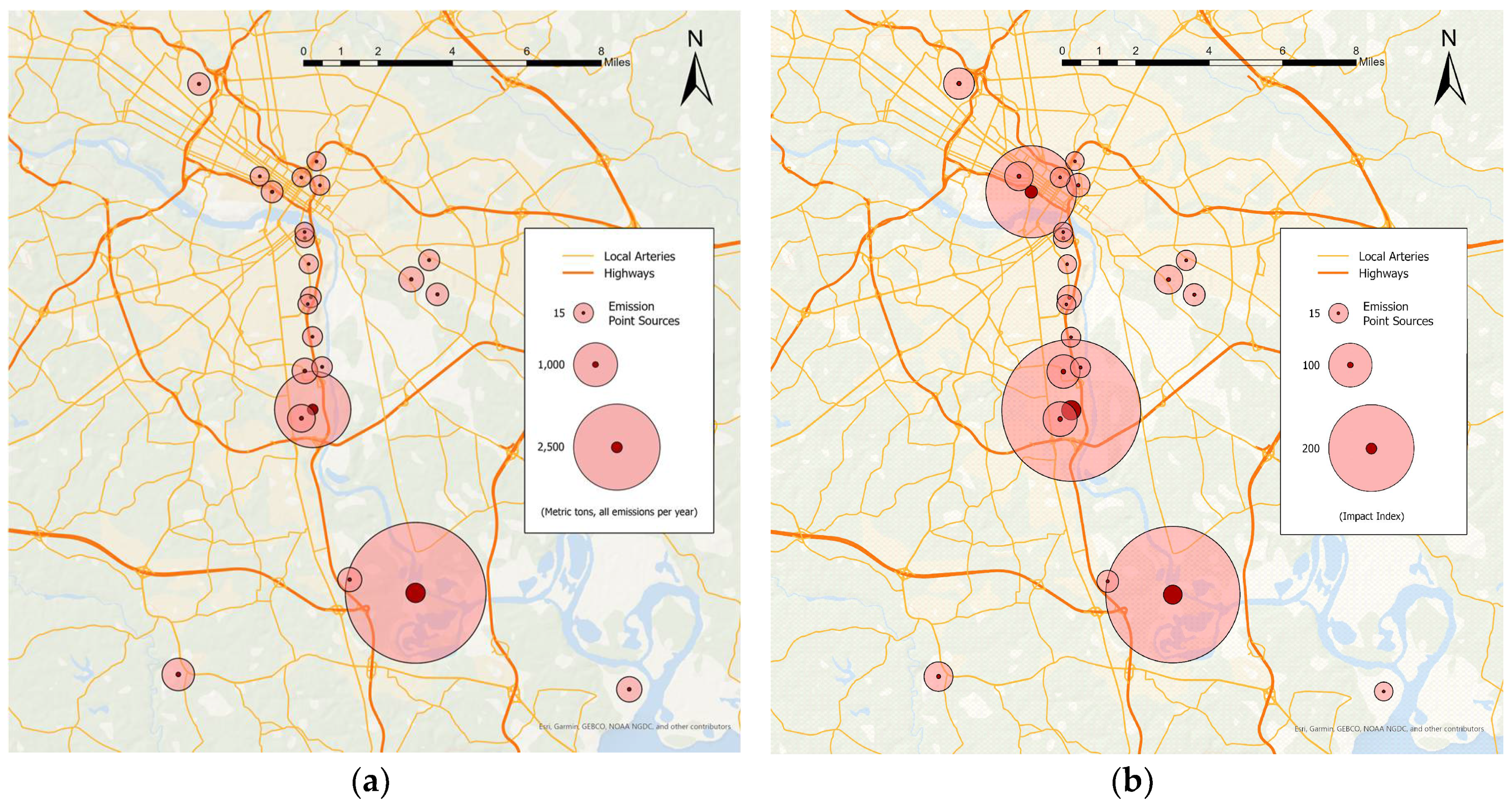
Figure 1. Twenty-three largest air pollution point-source emitters in Richmond, Virginia. Symbol size of each facility is proportional to (a) total emissions and (b) derived “impact index,” estimating the relative impact on Richmond’s urban core. Dark orange lines represent highways, and lighter orange lines depict other major roadways. Data represent post-2017 records obtained from the Virginia Department of Environmental Quality (DEQ).
Sustainability 12 10089 g001
Figure 2. Locations of eight PurpleAir sensors installed in Richmond, Virginia. Each is represented by a purple triangle with accompanying labels. The underlying polygons represent a vulnerability index by census block within the city limits. The color gradient depicts dark blue as high vulnerability and light yellow as low vulnerability. Labels represent sites for each sensor as follows: TLH = Todd Lookingbill’s house; URJ = University of Richmond Jepson School; WLO = Willow Oaks; VSN = Väsen Brewing; SMV = Science Museum of Virginia; CHL = Church Hill; MSI = MathScience Innovation Center; and NRC = Neighborhood Resource Center of Greater Fulton.
Sustainability 12 10089 g002
Figure 3. Variance among hourly average temperatures recorded by all eight PurpleAir sensors on the ten hottest days of 2019. (a) Distributions of temperature values by site are ordered left to right by mean and fall into five distinct categories of significant difference as indicated by colors. Green corresponds to lower average temperatures, while higher average temperatures are shown in orange. (b) These colors are projected onto the location of each site with an underlying vulnerability index.
Sustainability 12 10089 g003aSustainability 12 10089 g003b
Figure 4. Daily ≤2.5 μm particulate matter (PM2.5) averages plotted against daily temperature (°C) averages from February 14 to November 14, 2019. The overall trend exhibited a weak positive correlation (R = 0.35). However, a distinct cluster of consistently high PM2.5 values occurred on the hottest days of the year (depicted in red), while cooler days exhibited highly scattered PM2.5 readings. The mean PM2.5 values were significantly higher (t(9) = 3.89; p < 0.01) on the ten hottest days (10.10 μg/m3) than for the total 2019 record (7.60 μg/m3).
Sustainability 12 10089 g004
Figure 5. Average PM2.5 and temperature values from each of the eight PurpleAir sensors on the ten hottest days of 2019. Temperature and PM2.5 values on the hottest days of the year were highly variable among sites but correlated within sites.
Sustainability 12 10089 g005
Figure 6. Hourly PM2.5 averages from each of the eight PurpleAir sensors aggregated into a 24-h diurnal cycle for the ten hottest days of 2019. PM2.5 levels peaked in the early morning and reached their minima in the mid-afternoon. The variability between sensors at any given time of day is also visible.
Sustainability 12 10089 g006
Figure 7. Variance among hourly average PM2.5 values recorded by all eight PurpleAir sensors on the ten hottest days of 2019. (a) Distributions of PM2.5 values by site are ordered left to right by mean and fall into five distinct categories of significant difference as indicated by colors. Green corresponds to lower average PM2.5 concentrations, while higher average PM2.5 concentrations are shown in orange. (b) These colors are projected onto each site with an underlying vulnerability index.
Sustainability 12 10089 g007aSustainability 12 10089 g007b
Figure 8. Locations of eight original PurpleAir sensors plus 12 additional sensors that have been subsequently installed. The points are underlaid by a vulnerability index. Areas with the greatest need for future monitoring are outlined in red. These areas are among the most highly vulnerable in the city, both according to the vulnerability index and in their proximity to point-source emitters.
Sustainability 12 10089 g008
Table 1. Cross comparison of two co-located PurpleAir PA-II sensors (“MSI” and “EHN”) and a Teledyne 640X reference instrument using PM2.5 hourly averages ranging just over one year (10/10/2019–10/29/2020). Results from Spearman’s rank correlations (rho), Pearson’s correlation analyses (R), and linear regressions (slope) are shown. Inter-sensor correlations between PA-II channels and between the two PA-II instruments were very strong, while correlations between the PA-IIs and the T640X were moderately strong.
T640XMSI AMSI BEHN A
EHN Brho = 0.70rho = 0.99rho = 0.99rho = 0.99
R = 0.69R = 0.98R = 0.99R = 0.99
Slope = 0.83Slope = 1.04Slope = 0.97Slope = 1.00
EHN Arho = 0.69rho = 0.99rho = 0.99
R = 0.68R = 0.99R = 0.97
Slope = 0.82Slope = 1.04Slope = 0.98
MSI Brho = 0.68rho = 0.99
R = 0.69R = 0.99
Slope = 0.82Slope = 0.97
MSI Arho = 0.68
R = 0.67
Slope = 0.85
Table 2. Cross comparison of two co-located PurpleAir PA-II sensors (“MSI” and “EHN”) and a Teledyne 640X reference instrument using hourly PM2.5 averages with temperatures of >90 °F (32.2 °C). Results from Spearman’s rank correlations (rho), Pearson’s correlation analyses (R), and linear regressions (slope) are shown. Inter-sensor correlations between PA-II channels and between the two PA-II instruments were very strong, while correlations between the PA-IIs and the T640X were moderately strong.
T640XMSI AMSI BEHN A
EHN Brho = 0.61rho = 0.99rho = 0.99rho = 1.00
R = 0.53R = 0.98R = 0.99R = 1.00
Slope = 0.66Slope = 1.16Slope = 1.06Slope = 1.01
EHN Arho = 0.61rho = 0.99rho = 1.00
R = 0.53R = 0.99R = 1.00
Slope = 0.67Slope = 1.14Slope = 1.05
MSI Brho = 0.62rho = 0.99
R = 0.54R = 0.99
Slope = 0.72Slope = 1.08
MSI Arho = 0.62
R = 0.54
Slope = 0.78
Publisher’s Note: MDPI stays neutral with regard to jurisdictional claims in published maps and institutional affiliations.