1. Introduction
Air pollution is a rising threat to people’s health and the global environment. Based on [
1], the International Energy Agency (IEA) states that the premature death of approximately 6.5 million people every year is a result of air pollution. While people are increasingly aware of their health, air pollution issues in many countries remain unresolved, and world health risks will continue to grow over the next few decades. Any air material that may threaten or damage the human, plant, animal, and environmental life or cause undesirable changes is referred to as the air pollutant [
2]. Several sensing devices have been developed to track air quality in many countries all over the world. One of the essential air quality indicators used to define the relationship between air pollution and human health has been identified as the air pollution index [
3]. Air quality has become more critical in recent decades due to environmental health threats caused by high pollution rates [
4]. The weather forecast ensures sustainable social and economic development [
5]. In 650 BC, weather predictions started when Babylonians tried to predict the weather based on cloud observations [
6]. However, air pollution control is very complicated. Several researchers suggested different theories of forecasting. However, these theories have not been sufficient. Therefore, it was clear that weather from a broader perspective must be understood. Measurements of the atmosphere were carried out with the invention of new instruments. Different tools, such as telegraphs and radiosonde, enable better weather monitoring [
7]. These tools are currently used for recording weather changes. These pollutants can be produced as solids, droplets, or gas molecules [
8]. Events of air pollution are primarily caused by human activity.
production in Malaysia in 2000 was
metric tons, more than the global average of
metric tons [
9]. Air pollution becomes a public concern [
10]. The Department of the Environment is responsible for providing public information on environmental air quality based on API information. API is a basic method to explain air quality and provide easily understandable information on air pollution. Main pollutants consist of five subsets: sulphur dioxide
, particulate matter
, carbon monoxide (CO), nitrogen dioxide
and ozone
[
11]. The dynamics of air pollution are generally expressed by various factors, such as temperature, moisture, wind directions, wind speed, etc. The API data available in Malaysia are measured by the American model, where each pollutant value is from 1 to infinity [
12,
13].
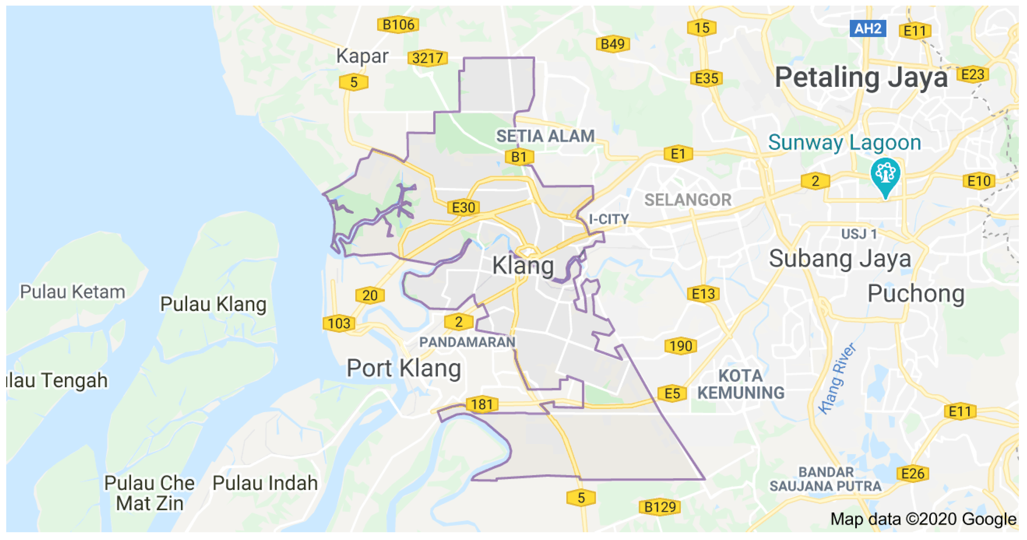
Figure 1 shows the location of air pollution monitoring stations. An API value below 100 corresponds to good air quality, and an API value above 100 indicates higher air pollution. API knowledge will enable public authorities, policymakers, and individuals to establish plans to mitigate the effects of air pollution events [
14].
To summarize, API forecasting is a crucial development issue. In this paper, a deep learning model based on One-Dimensional CNN and Exponential Adaptive Gradient optimization is proposed to forecast future API concentration. Four measurement indices, MAE, RMSE, MAPE, and , have also been used in the experiments to evaluate the overall performance of the proposed model. On top of that, other traditional machine learning algorithms, such as LSTM have been used for model comparison. As for the aspect of dataset selection, the Klang API dataset has been used.
2. Related Work
Several researchers have studied air pollution problems in Malaysia. Many studies have been carried out in recent years to measure air quality. Records of air pollution can be made early. Statistical methods, shallow machine learning models, regression techniques, least absolute shrinkage and selection operator (LASSO), elastic net, regression tree and regression forest are the most used to solve air-quality prediction problems [
15,
16,
17,
18,
19]. Many scientists have tried to use the neural network to predict future air quality [
20,
21,
22]. Deep learning methods have become an active research field in recent years for prediction of air quality, with Convolutional Neural Network (CNN) [
23], Recurrent Neural Networks (RNN) and their variants have been widely used [
24,
25]. RNN models, such as Long Short-Term Memory (LSTM) have been applied to forecast air quality, especially with different data samples. A very complex LSTM neural network model will have an enormous predictive potential [
26,
27,
28,
29,
30,
31,
32]. In addition to deep uncertainty [
33], Manifold Learning [
34], and Gated Recurring Unit (GRU) [
35] have recently been used and work well on air pollution forecasting. Moreover, the manifold learning method, deep belief network [
34], and encoder-decoder model [
36] have been also widely used for air pollution forecasting. Both traditional and modern methods can investigate and forecast API trends. The decision-making process in air quality policy can be considered significant.
Deep learning [
23,
37,
38] is a type of machine learning that trains computers to perform human-like tasks. It is characterized by a multi-level hierarchical architecture with subsequent stages in information processing [
39]. Deep learning has two types, Recurrent Neural Networks (RNN) and Convolution Neural Networks [
23]. CNNs are most frequently used with two-dimensional data, such as images [
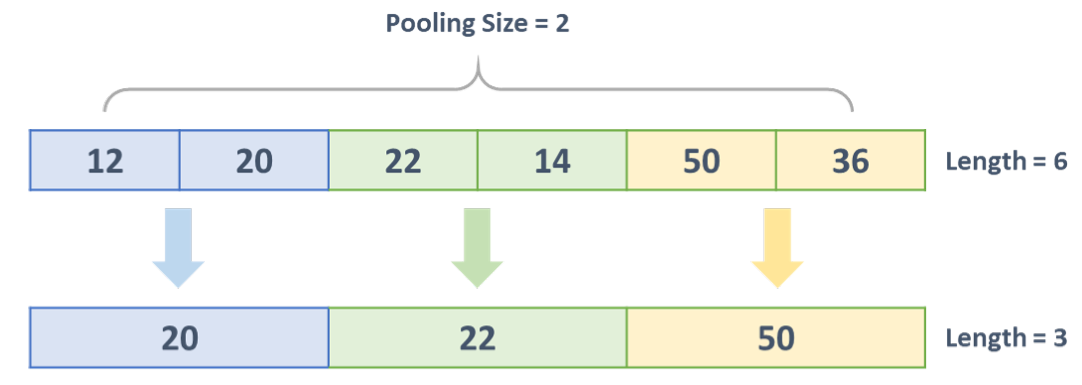
40]. They are made of at least one hidden layer and a fully-connected layer that is connected to the other network layers, and each layer contains weights. The hidden layers are typically consisting of convolution, pooling, and fully-connected layers [
23,
38]. The network architecture of CNN was mainly designed for 2D data processing. CNNs achieve greater performance with image processing and speech recognition than other deep learning architectures [
41]. However, recently, CNN has been widely used as a modelling framework for time series data with multiple variables [
39] where layer by layer sparse processing and extraction is carried out by multiple convolution pooling layers [
42]. As an alternative, a modified version of 2D CNNs, called 1D Convolutional Neural Networks (1D-CNNs), has recently been developed [
39,
43,
44]. In many applications, 1D-CNNs are advantageous and thus preferable to their 2D counterparts in dealing with 1D signals due to the following reasons: (1) computational complexity of 1D-CNNs is significantly low; (2) with relatively shallow architectures, 1D-CNNs are able to learn challenging tasks involving 1D signals; (3) 1D-CNNs are suited for real-time and low-cost applications due to their low computational requirements. A regular error back-propagation algorithm can be applied to train the CNN networks [
23]. It is easier to train CNNs because they have much fewer optimizing parameters than other standard deep and unidirectional neural networks [
45]. Rather than using hand-crafted features, deep learning methods, specifically CNNs, provide a structure in which both (feature extraction and prediction) are performed together in a single body block, unlike other traditional methods. The deep learning method is capable of learning useful characteristics from input signals [
39]. According to studies mentioned above, CNN accuracy increased faster than other time series prediction approaches, such as LSTM, which is gradually continued to improve slightly due to its nature procedure, which does not make it sufficient for real-time applications and computational cost.
5. Results and Discussion
One Dimensional CNNs are particularly promising in time series predictions since they can map the input to output sequences with past contexts in their internal state. They can be described as several copies of the same neural network. They transmit information to their successor and form a chain-like architecture, which is naturally connected to the sequences [
91]. Moreover, 1D-CNN combines both feature extraction and prediction into one learning body-block, which solves the problem of handcrafted feature selection in other networks, thus maximizing prediction performance. The proposed architecture and hyper-parameter selection, based on cross-validation and grid search, can be shown below in
Table 1.
Experiments have shown that the number of filters has a significant impact on feature extraction.
Table 2 shows the multi-convolution of the same input against various numbers of filter sizes. We can see that, as the number of filters increases, the accuracy also improves. However, the improvement comes at the cost of computational time.
Table 2 shows the model performance under a different number of convolution filters. The performance of the proposed model was empirically improved by determining the optimal filter size in the range of 64 and 128. Moreover, overall performance was best using 64 filters for all developed models since it gives satisfactory results with less computational time.
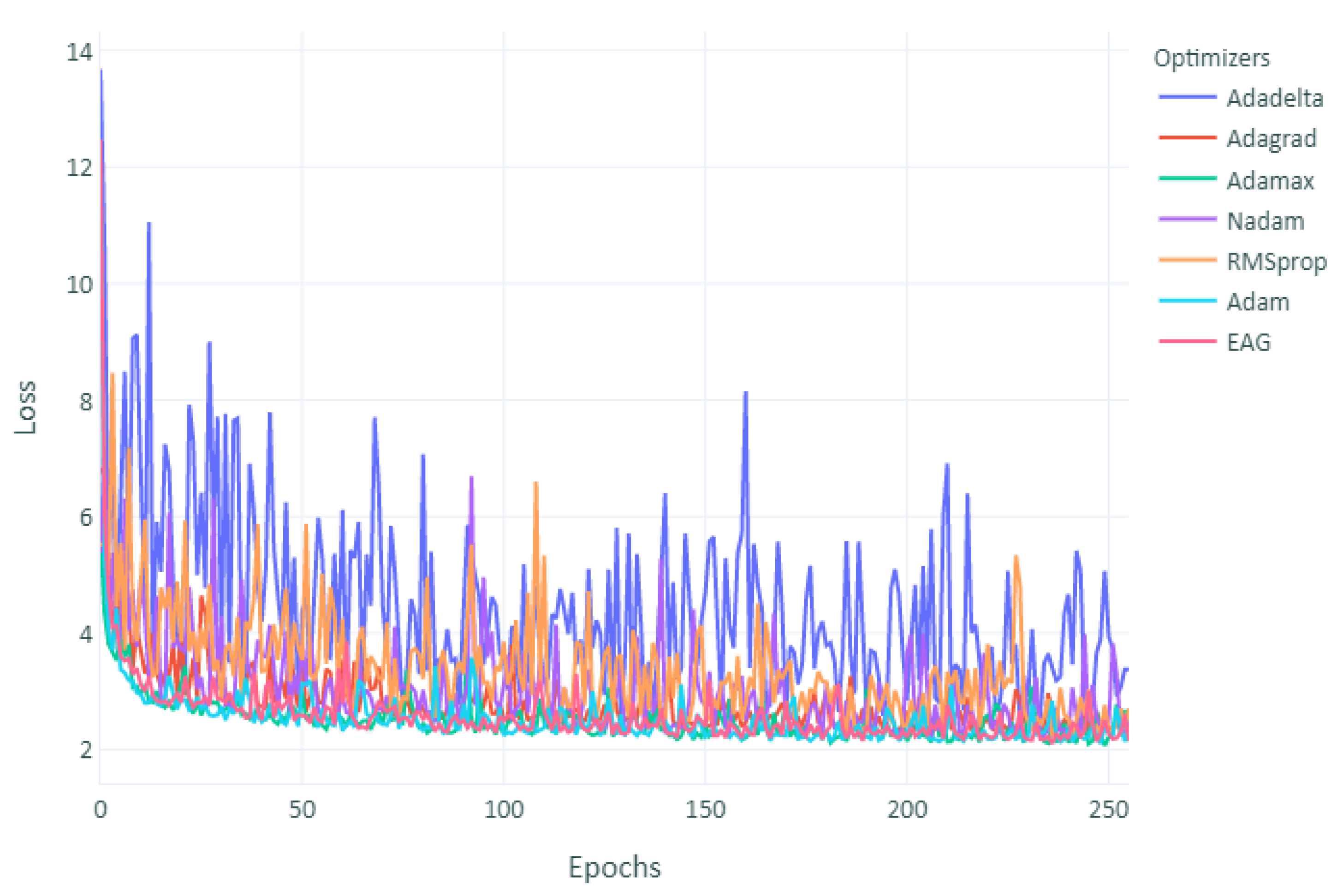
As can be observed in
Figure 5, despite the initial fast convergence of Adam, their final loss could not catch up with EAG. However, other optimizers converged faster than EAG but yielded similar performances. As observed, although Adam was fast at the beginning, its test accuracy stagnated after the second learning rate decrease. RMSprop performed even worse than Adam. On the other hand, EAG converged without increasing the loss in most of the runs. However, more time consumed, as shown in
Figure 5 and
Figure 6.
The selected network loss function (MAE) has shown that the training dataset loss function is not much lower than the validation dataset loss function, meaning that network did not overfit during the training process. Since we are focusing on one dimensional CNN and it is performing against counterparts approaches, such as LSTM, a network of other architecture was designed for efficiency comparison of the proposed system in the related domain [
6]. The outcomes of the comparison results can be shown in
Table 3.
Different optimizers have been selected to optimize the developed model. The performance and outcomes are displayed in
Figure 5 and
Figure 6. Adaptive optimization algorithms, such as Adam and RMSprop, in many cases, have shown better performance. Recent studies, however, indicate that generalization performance is often worse than SGD, especially for deep neural networks. Adam and RMSprop have shown a great result in a few runs and unsatisfactory performance in other runs. However, the lack of generalization performance of adaptive methods, such as Adam and RMSPROP, might be caused by unstable or extreme learning rates and suggested that the modest learning rates of adaptive methods can lead to undesirable non-convergence [
74]. Adam algorithm was found to be the best optimizer in terms of speed but not error rate. In addition, the hyperbolic tangent activation function generated better models than the sigmoid activation function in the output layer.
Table 4 shows the MAE, RMSE, MAPE, and
overall results obtained by both approaches—LSTM and developed 1D-CNN. The generated 1D-CNN model revealed an average of MAE of 2.036, RMSE of 2.354, and
of 0.966 over the test dataset for 25 independent iterations. The fitness of the developed model 1D-CNN was optimized by EAG and gave excellent and stable results in all iterations with the lowest average error rate compared to other optimizers. The prediction results are displayed in
Table 4. EAG was selected with a learning rate of
based on grid search as a primary optimizer for the developed models.
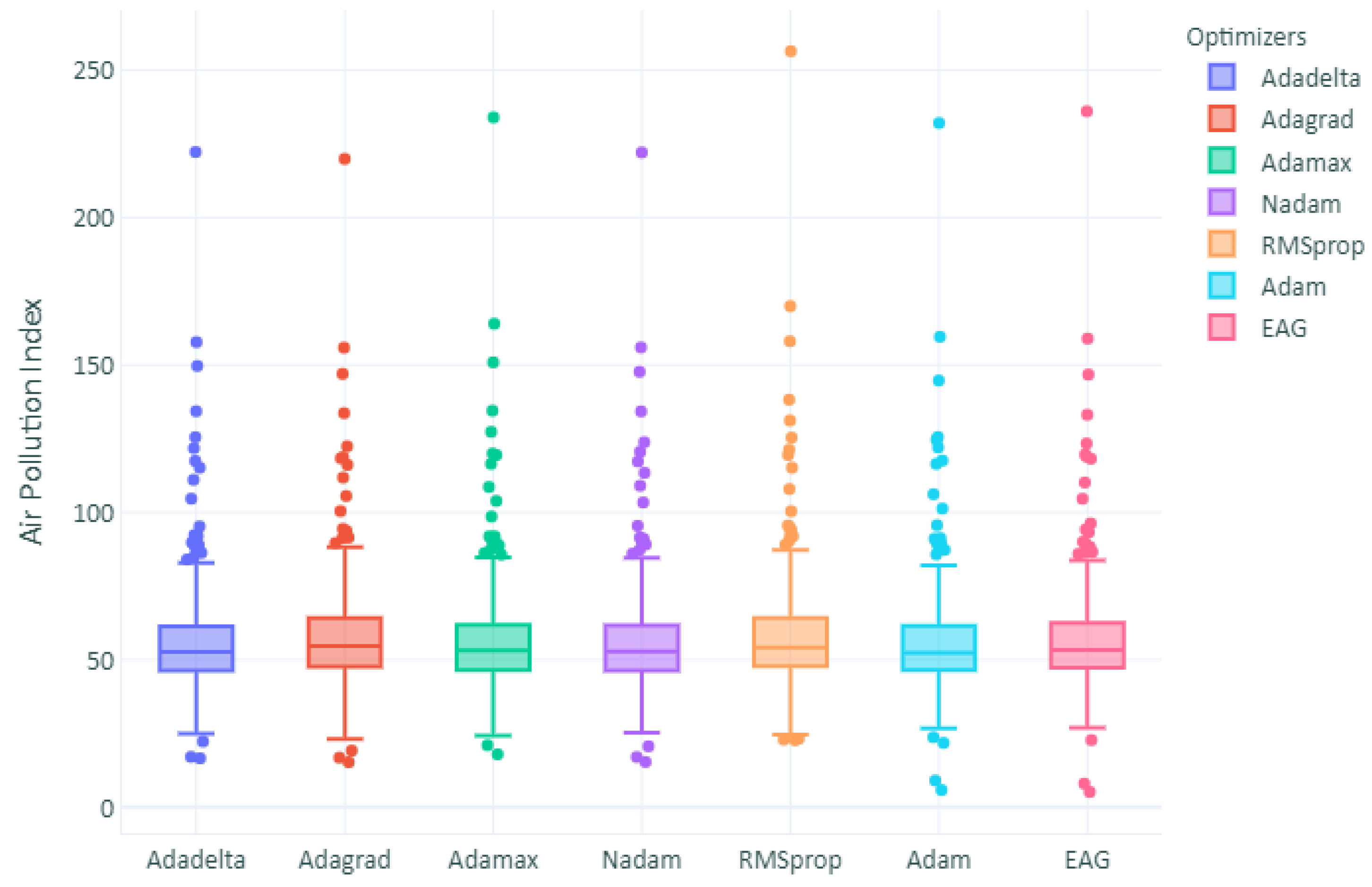
The boxplot of the prediction deviation is shown in
Figure 7. The height of the box partly reflects the fluctuation in the deviation data, and the flatter the box, the more centralized the data are.
Figure 8 represents the absolute difference between actual and forecasted values for each prediction model. The number of outliers in the other optimizers and the LSTM model was higher than the number of outliers in the 1D-CNN model. This can be referred to as the high RMSE obtained. In terms of the comparison analysis, the proposed method outperforms other models, including mainstream approaches, such as LSTM, not only in terms of performance but also time complexity and consistency. It fully proves the effectiveness and superiority of the 1D convects in non-convex optimization. We have demonstrated that the non-convex optimization performed better in all 25 independent runs, unlike other optimizers that have shown a big difference in MAE and RMSE in every run, since adaptive methods tend to converge quickly towards sharper minima. In comparison, flatter minima generalize better than sharper ones. However, we observed that the solutions found by adaptive methods generalize worse (often significantly worse) even when these solutions have better training performance. Therefore, as a part of future work, ensemble techniques could be investigated to combine each optimizer’s efficiencies with building up a super model.
Similarly,
Table 4 shows the four measurement indices for each model. The RMSE value of the proposed 1D-CNN–EAG model is lower than the models. The MAE and RMSE values of both Adam and RMSprop models are slightly lower than that of LSTM models, which can be clearly shown in
Figure 9a,b. It represents the values of RMSE of each optimizer and show that EAG has the lower average by far than that of other optimizers. In terms of training time and complexity, 1D-CNN is three times faster on average for every epoch. LSTM could not keep up the same performance in training time comparison. The average 1D-CNN time was approximately 4–7 s for every epoch, while LSTM took roughly 18–27 s for one epoch.
To compare the prediction effect of each model more intuitively, the scatter plots of observed and predicted API concentrations during the whole test set are illustrated in
Figure 10. The distribution between predicted and observed values can be seen in
Figure 10a,b. Apparently, variants of 1D-CNN (
Figure 10b) show better results than LSTM (a). Compared with all the models described above, the proposed model is more sensitive to sharp changes. Which mainly attributed to the existence of convolution networks that capture richer local change information. API was correctly forecast on most peaks, especially in days with very high averages with a good RMSE value. We investigated the influence of epoch size on various models. By increasing iterations, the model loss gradually decreases, and MAE reaches its lowest at the value of 1.894 at all experiments runs, as shown in
Table 3.
Checkpointing has been utilized to save the network weights only when there is an improvement in the validation dataset. The weights are stored in a file if and only if the validation accuracy improves. It will ensure that the best model is saved. Moreover, all models used the early-stopping condition that stops and interrupts the training if the validation loss on the validation information does not change in 12 epochs of training. We also observed that model error remains unchanged as the lookup size increases. Finally, results have shown that 1D-CNN and EAG optimizer can learn complex patterns better than other predictive models. From the above results, we have demonstrated that a 1D-CNN–EAG can successfully predict the API. Prediction for API time series under different experimental conditions has been carried out. Although the EAG optimizer obtained the best results, performance in terms of time complexity was observed. Certain functions with minor changes to our proposed 1D-CNN–EAG architecture may also be appealing to many other domains.
It has been demonstrated in many applications that 1D-CNNs are relatively easier to train and deliver minimal computational complexity while achieving cutting-edge performance, especially now with convergence in both the convex and non-convex settings. This paper demonstrated the benefits of utilizing machine learning techniques for predictive analytics that will create enormous opportunities for having deeply beneficial influences on society (healthcare, education, sustainability, etc.). Additionally, this method could be applied to other contexts in different countries. We are optimistic that researchers and public agencies can continue to expand and test this method to improve environmental sustainability.
The obtained network training dataset is the key downside of the neural network. Suppose training data are insufficient and not appropriate. In that case, the network will quickly learn the dataset bias and generally make poor predictions of data with trends the training data have never seen. Besides, it is typically more difficult to track back if a network does not function as intended. We have used only the data provided in this paper for network training, which may lead to bias by overlooking the effects of unusual situations. Perhaps a more effective approach would be used to train the network in a semi-supervised fashion to boost network performance on unseen data by using limited actual data and data generated during the training. It will also increase data from different sectors, such as transportation and industry, on air pollutants to improve the learning model. This will be used in our future research topics [
92].
Future work will focus more on effective methods to adjust hyper-parameters and the use of feature selection [
92,
93]. It will help to remove redundant features and thus obtain better performance. Additionally, future work will investigate more accurate methods of hyper-parameter tuning techniques. Although the grid search can be utilized, the search range needs to be manually updated since values are always fixed. It will be important to find an adaptive way to automatically adjust the hyper-parameters searching process and make the neural network architecture evolve by automatically reshaping, adding, and removing various layers. Additionally, this work will consider hybrid networks [
94] to merge the advantages of different approaches.

 ,
, 


