Abstract
The purpose of this paper is to study how advanced information about customer needs obtained through an Advance Purchase Discount (APD) contract can be exploited to coordinate the capital flow and enhance the efficiency of a two-stage supply chain (SC) under decentralized control in cases of stochastic customer demand. We developed an APD model in the form of an option contract, where the model and evaluation include the flexibility for the upstream firm to decide whether to provide a discount for an advance purchase at its own discretion. Applying the model to a Fortune 100 company, a leader in the Fast Mover Consumer Goods (FMCG) industry, showed that under certain conditions, and with suitably chosen contract parameters, management of decentralized control via APD contracts can lead to system-wide efficiency, and the individual decision makers pursue their own best interests, ensuring a win-win condition.
1. Introduction
The aim of supply chain management (SCM) is to coordinate material, cash and information flows along the supply chain (SC) from an end-to-end (E2E) perspective, i.e., from suppliers to consumers [1,2]. SC control may be either centralized or decentralized [3]. Centralized control involves the presence of a single decision-maker who is in possession of all the information pertaining to the SC, managing it in its entirety, and thus, who is able to optimize the performance of the whole system (channel coordination). Decentralized control involves the presence of several decision makers (SC actors), each taking decisions in pursuit of their own probably conflicting goals [4]. While centralized control ensures the system’s efficiency (channel coordination), in decentralized systems, locally rational behaviors result in the overall inefficiency of the SC [5,6,7,8,9,10,11,12,13,14,15]. Both academic researchers and practitioners have focused on trying to find coordination mechanisms that can eliminate such inefficiency by driving local actors to behave in the interests of the global SC rather than their own. This problem is known as “alignment of incentives” in decentralized SCs [16]. Supply chain contracts are proposed as mechanisms which are capable of aligning incentives in SCs [17], and are based on transfer payment schemes that regulate how savings can be split and risks distributed fairly among all the actors in the SC chain [2,18,19,20]. In particular, the general aim of SC contracts is to establish rules for materials accountability and/or pricing that will be able to guide autonomous entities towards a globally desirable outcome [5]. SC contracts are therefore based on the principle of improving the benefits for all the parties involved compared with what would happen if there were no such contract (i.e., the so-called win-win condition). Conversely, if the win-win condition were not satisfied, the SC actor would not be prompted to adopt the contract [3]. In this sense, SC contracts are considered one of the operating models of Supply Chain Finance (SCF), together with purchase order financing, factoring or reverse factoring, inventory financing, and so on [21,22,23,24]. In capital-constrained supply chains [25,26], SC contracts are an effective means which can be used in the Supply Chain Finance (SCF) systems to coordinate the capital flow and enhance the efficiency of supply chain [27,28,29]. Different from the traditional fixed-asset-based financing, SCF is a real-trade-based short-term financing service [23].
Various contract types have been designed to align the incentives of SC members along the SC to drive optimal action within the SC. These include quantity flexibility (QF) contracts (2), backup agreements [30], buy back or return policies [28,31], incentive mechanisms [32], revenue sharing (RS) contracts [33], allocation rules [34], and quantity discounts [35].
Little research has been dedicated to the Advance Purchase Discount (APD) contract as a supply chain coordination mechanism. Using ADP, the firm offers its downstream retailers an opportunity during the sales season to place an additional order in advance at a discounted price [36]. Advancing some of the retailer’s demand, an APD incentivizes the communication of accurate information from downstream tiers at a time chosen by the firm, which improves capacity planning and investment [37], and transfers some of the mismatch risk to the retailers [38,39]. Most of the literature has focused on APD programs that retailers offer their customers [40,41,42] without considering the benefits that an APD may have in terms of channel coordination and ensuring win-win conditions for the actors along the SC. On the other hand, industrial practice widely applies contracts of this type to obtain supply chain benefits (for example, [43,44]). These considerations have led us to try to address this research gap.
The purpose of this paper is to study how advanced information about customer needs obtained through an APD contract can be exploited to coordinate the capital flow and enhance the efficiency of a two-stage SC under decentralized control in cases of stochastic customer demand. Under certain conditions, with an appropriate choice of contract parameters, handling decentralized management via an APD contract can bring about system-wide efficiency, while the individual decision makers follow their own best interests, ensuring the win-win condition.
The paper is organized as follows. Section 2 provides a brief review of the relevant literature, while Section 3 proposes a model based on an ADP contract for the coordination of a two-stage SC. Section 4 examines numerical application to the real case of a Fortune 100 company in the FMCG. Some final remarks close the paper.
2. Literature Review
2.1. The Advance Purchase Discounts Literature
This paper is closely related to the literature on the APD contracts.
APD contracts were first studied as direct offers from a retailer to consumers in the market [44]. Cachon et al. [34] considered an “advance booking discount” (ABD) program that entices consumers to commit to their orders at a discounted price prior to the selling season, which shifts some of the demand to an earlier time and enables retailers to better manage both inventory and capacity.
Further studies focusing on consumer APD contracts have extended these models, taking into account the competitive nature of retailing to analyze APD programs in competitive conditions [45]; others have used them as a price discrimination mechanism [46,47,48,49], and yet others analyzed the benefits of adopting APD programs together with other programs such as Revenue Sharing [50]. On the same topic (consumer APD contracts), Li et al. [40] investigated the best seller’s strategy choice on the basis of the relative sizes of heterogeneous consumer segments; Nasiry et al. [41] analyzed the effect that an APD contract may have on a firm’s profit according to consumer buying behavior; Yu et al. [42] investigated the relationship between advance selling, a seller’s quality signaling strategy, and a firm’s profit.
Of greater relevance to our study is the literature on APDs offered in a supply chain. While the APD contract offered to actors in the supply chain is similar to consumer APD contracts, actors in an SC are typically assumed to have different utility and incentive structures from those of consumers, which leads to significantly different analyses and implications [38,44]. In particular, new issues, such as risk and profit sharing among SC actors and incentive coordination, that are not relevant in consumer APDs, play an important role in these settings. The pioneering works by [38,51,52] were the first to identify these effects. In particular, Donohue [51] examined the problem of developing supply contracts which encouraged the proper coordination of forecast information and production decisions between a manufacturer and distributor of high fashion and seasonal products. Cachon [38] studied how the allocation of risk via these SC contracts impacted on SC efficiency. Ozer et al. [52] proposed a kind of APD contract that they called “dual purchase contract” to mitigate the adverse effect of the wholesale price contract by analyzing how and when a dual purchase contract creates strict Pareto improvement with respect to a wholesale price contract.
The contribution of our study in relation to the existing literature on APD contracts is that we study how this contract can be exploited to coordinate a two-stage SC under decentralized control with stochastic customer demand in such a way as to bring about a win-win situation. Under certain conditions, with an appropriate choice of contract parameters, organizing decentralized management by means of an APD contract can bring about system-wide efficiency, while the individual decision makers follow their own best interests, thus guaranteeing the win-win condition.
2.2. Literature on Option Contract Modelling
Let us consider a standard wholesale contract between the upstream firm and its downstream retailers: once the contract is established, the firm must supply the goods at the agreed price, regardless of the market conditions at each point in time. Furthermore, once the retailers have agreed to purchase the goods, they cannot reconsider the purchase, e.g., if the demand does not materialize.
With the APD program, on the other hand, the firm has the right (without the obligation) to decide, at each specified interval during the contract, whether to sell its products at a discounted price to retailers who advance their orders in the time period between intervals.
Operationalizing a contract of this type requires modelling the managerial flexibility of the upstream firm to choose whether to offer the discount on the basis of the current market conditions (i.e., actual demand by retailers who may decide to advance their orders) and SC savings obtained through increased visibility due to the APD program. Traditional approaches, such as those based on Discounted Cash Flows (DCF) analysis (especially NPV), cannot be used to model this managerial flexibility. Consequently, they cannot be used to price the value of the investigated APD contract. They implicitly assume that a strategy or project will be undertaken now and operated on continuously on a set time scale, until the end of its expected useful life, even though the future is uncertain. Therefore, they are “static” and underestimate the upside value of the investment [53] by assuming management’s passive and inflexible commitment to a certain “operating strategy”. They are also “deterministic”, since they make implicit assumptions concerning a certain “expected scenario” of cash flows. In the real world, the actual cash flows will probably differ from what management originally expected because of uncertainty and competitive interactions. As new information is available and uncertainty about the market conditions and future cash flows is gradually resolved, management should revise the operating strategy it originally anticipated in order to achieve the initial desired goals [54]. As a result, traditional managerial techniques that arose from stable environments are in crisis as they are unable to grasp the value of flexibility for changing operating strategy to capitalize upon favorable opportunities or to cut losses in the event of adverse development [55]. A better valuation approach to support decision making in uncertain environments should, in fact, incorporate the uncertainty and active decision making required for a strategy to succeed [56]. Hence, it is essential that flexibility be quantified, and any attempt to do so almost naturally leads to the concept of options [57]. From this perspective, the APD contract, which provides upstream firms with the possibility of deciding to offer a discount to those retailers who advance their orders, adopts an option mechanism.
This paper is closely related to the literature on the use of options in SCM. Research on this aspect has mainly focused on two branches: economic efficiency derived from options, and operational flexibility [58].
Concerning the first, Newbery [59] set out a model consisting of a forward and a spot market for electricity. Spinler [60] discussed the implications of an options market scenario for electronic transportation platforms. Spinler et al. [61] and Wu et al. [62] developed models to value contingency contracts in the presence of demand, cost and price uncertainty, and demonstrate that economic efficiency can be enhanced in a market set-up consisting of an option contract and a spot market rather than a pure spot market.
As for the operations management literature, Barnes-Schuster et al. [63] studied how options provide managerial flexibility in response to uncertain market changes and how to achieve channel coordination by options based on a model of two periods with correlated demand. Ref. [30] considered a backup agreement, which is essentially an option contract. Milner et al. [64] and Wang et al. [65] explored the bidirectional option from the buyer’s perspective whereby the option buyer can freely adjust the quantity of the initial order both upwards and downwards. Cheng et al. [66] considered an option model where the option buyer, in addition to a committed order quantity, also has the right to acquire an additional quantity of the supply, if necessary, by purchasing options from the supplier. More studies on the use of options can be found in [58,67,68].
We are unaware of any research that specifically models APD as an option contract, thus addressing the benefits for the supply chain when, under an APD contract, upstream firms have the possibility. but not the obligation, to give downstream firms incentives (i.e., a price discount) to make an earlier commitment to purchase. In other words, to the best of the authors’ knowledge, there are no studies that take into account the flexible behavior of the upstream firms ensured by such contracts. This is an important issue when studying the APD as a coordination mechanism and when fine-tuning the contract parameters to ensure successful application of the contract itself. In fact, failing to consider the flexibility of the upstream firms to decide when and whether to offer a discounted price for advanced orders means effectively neglecting the mechanism of such contracts, and as a consequence, overestimating or underestimating the value of the APD benefits. In turn, an incorrect estimation of APD benefits means being short sighted about both the advantages and limitations of such contracts, thus undermining the success of their application. For example, the APD is often recognized as a way to improve the manufacturer’s ability to invest in new technology or justify equipment purchases, since it overcomes the limitations of last-minute ordering under a wholesale contract [52]. Correct estimation of the APD benefits is a requirement if the manufacturer’s ability to invest in new technology is to improve. Furthermore, an upstream firm that chooses to adopt an APD often incurs a fixed cost for implementing and promoting the program. Therefore, an accurate valuation of the benefits of an APD is needed to understand whether the program is worth its costs. Lastly, once the firm has launched the program with the downstream clients, even though the firm may, but with no obligation to do so, offer a discounted price to those that advance their orders, it may prove detrimental to the relationship not to make the offer because it does not seem advantageous. The firm has to carefully assess a priori whether it is in its interests to launch an APD program.
The above discussion offers a strong incentive for us to model the APD as an option contract in the coordination of a two-stage SC faced with a stochastic customer demand, including the flexibility of the upstream firm to decide whether to provide a discount for an advance purchase at his or her own discretion (that is, only when economically worthwhile) in the model. This will allow a correct analysis of the general conditions under which the APD program is beneficial, i.e., this approach is able to bring about supply chain coordination and a win-win situation, as well as an understanding of the impact of contract parameters (discount price, pre-booking time, etc.).
Regarding option pricing, the methods traditionally proposed in the literature on real options are financially-based approaches to option pricing [69,70,71,72,73]. However, they often turn out not to be workable in practice [74,75]. Because of their origins in finance, many of the required assumptions are not respected in the real world. For example, most of the traditional methods are one/two factor models, i.e., they assume that only one/two inputs are uncertain.
Simulation-based research is preferred for complex and expanded problems with several factors and interactions. Simulation is able to incorporate random occurrences into the system to estimate their effects. Changes to the underlying simulation model or inputs can be made to answer “what-if” questions while always keeping complete control of the system [76]. In this sense, computer simulation becomes an attractive way to understand system behavior when “real life” controlled experimentation with logistics and supply chain systems is extremely difficult [77]. The stochastic nature of supply chains and the complexity of the interactions within them justify the successful application of simulation to supply chain settings [76,78,79,80,81].
3. The APD Model
Consider a supply chain consisting of a supplier S who provides a short life cycle product to retailer R, who in turn serves the market demand. This may be the case of fast-moving consumer goods and products with seasonal demand (e.g., fashion wear, toys, seasonal sports goods). The SC is characterized by decentralized control, namely each SC actor makes decisions by optimizing his own objective. In particular, supplier S chooses the unit price at which to sell the product to the retailer, and the retailer R decides the order quantity, with both maximizing their own profits.
Under the APD contract, the supplier may decide period by period whether to offer a discounted price to a retailer who advances its orders. This choice is based on an evaluation of cost and benefits associated with that choice. If the supplier offers a discount, the retailer will make a saving for ordering in advance. This is not an obligation for the retailer, but a choice.
To achieve channel coordination, the two independent decision-makers should act in such a way as to maximize the SC total profit given by ΠSC, calculated as in (1). The APD contract is a coordination mechanism offered by the supplier to the retailer, which modifies the retailer’s profit and also that of the supplier so as to incentivize them to make decisions leading to total optimization of the SC.
where ΠS is the supplier’s profit during the selling period due to the implementation of the APD program, and ΠR is the retailer’s incremental profit. In both cases, we calculate the profits as the differential profit compared with the base case in which the APD is not implemented.
We assume that each decision maker acts in such a way as to maximize his/her profit. In particular, from the supplier’s standpoint, we can say that the APD program gives the supplier the right, without the obligation, to decide on the periods in which to sell products at a discounted price to retailers who advance their orders, incurring additional administrative, handling, and monitoring costs Co, generated by this contract rather than simpler contracts, such as wholesale price contracts [38]. These are sunk costs since they are charged to promote and manage the program without the retailers knowing whether the APD program will be fully exploited. According to the real options’ terminology, Co may be interpreted as the cost of the option. At each specified interval, the supplier chooses whether to offer a discount for the retailer’s orders placed in advance in the specific period between intervals; the decision is open at each interval during the duration of the APD contract. Such a scheme allows the supplier to gain “supply chain savings” because of improved trade terms, against some “revenue losses” (selling products at a discounted price). This option mechanism can be modelled as a real (Australian) put option held by the supplier, which gives the owner of the option the faculty to sell the underlying asset at the exercise price. An Australian option is a claim that can be redeemed M times, M > 0, at different stopping times t (t ∈ [0, T]) chosen by the holder of the claim [82]. In our case, at specified intervals within the time horizon of the validity of the APD program (t), the supplier will have the right to engage the retailer in advance purchases by offering an agreed discount for the subsequent period. The retailer still has the faculty to not advance orders, as the industries where APD may be applicable are usually characterized by very collaborative supplier-retailer relationships. In terms of real options, the owner of the option is the supplier, the “revenue loss” can be interpreted as the stock price, St, and the “supply chain savings/benefits” will be the exercise price of the put option, Xt. During the short time horizon of validity of an APD program (typically T is the year), at any time t (typically the month) prior to the end of the time horizon, to maximize profit, the supplier would engage in the APD program if the supply chain benefits (Xt) are higher than the revenue losses (St), and the related payoff at each t is calculated as in (2).
The underlying asset of option St, namely revenue losses, can be quantified as St = K × P × Qt.
- K is the price discount offered to the retailer on the original regular price P for each unit of the product ordered in advance, where K ∈ (0, 1]. By purchasing the product in advance, the retailer obtains a price discount and guaranteed product delivery. Let TAPD be the preselling time, namely how much time in advance the product can be bought. Generally, K depends on TAPD since different discounts and price tiers may exist for different TAPD. For the sake of simplicity, we assume one single value for TAPD (as per standard industry trade terms), and therefore one value for discount K. Regular price P can be assumed to be deterministic since it is generally fixed at the beginning of the contractual relationship and does not vary in the short time horizon of validity of an APD program (here we assume 1 year).Dt is the total (stochastic) demand of the product that is sold to the retailer at t (i.e., the agreed amount under a standard contract).
- Qt is the total (stochastic) quantity of the product sold under the APD scheme at t to those retailers who agree to advance their orders and subscribe to the APD program for the product in question. Qt is a stochastic variable since it is not known how many orders will be made under the APD program. Also, Qt is generally less than Dt (the total demand under a standard contract) since the usual contract setting assumes that the retailer has the faculty to not make the order early and not exploit the discount offered by the upstream firm.
According to (2), at each t the supplier will decide whether to engage in the APD program (ωt = 1), or not (ωt = 0). The total number of times the supplier engages in the program within the time horizon T is calculated in (3).
The exercise price of put option “Xt” in Equation (2), which represents the benefits of the APD program at time t, is calculated as differential benefits in comparison to the base case with no APD program. We assume that these benefits are mainly due to SC savings obtained through increased visibility thanks to the APD program. In particular, given that the supplier’s decision maker may act at two levels, the operational level (i.e., decisions related to manufacturing and logistical activities in order to meet the retailer’s requirements) and the chain level (all the bids from potential suppliers are evaluated and the final configuration of the supply chain is determined) [83], when more time is available for producing the product, thanks to the APD program, it may be used to reduce costs at the operational level (for example, by reducing the cost of crash production after the due date and the penalty cost incurred for late delivery) or at chain level (for example, by choosing alternative transportation options or suppliers that are cheaper but slower). For the sake of simplicity, we assume that when more production time is available thanks to the APD, the supplier uses that time first to improve activities at the operational level and then those at chain level. Of course, this assumption could easily be released by seeking the trade-off between these two strategic choices. This is, however, beyond the scope of the current paper.
The operational benefits produced by an APD program mainly refer to the areas of Manufacturing and Operating Expenses (MOE) and Inventory Costs (IC); the benefits produced at chain level concern Transportation and Warehousing (T&W) costs.
As regards the benefits due to savings in Manufacturing and Operating Expenses (MOE), we calculate them as the difference between MOE under “standard” conditions (with no APD program) and MOE under an APD program. As APD programs allow the supplier to know the demand in advance, they increase supply chain visibility and, as a consequence, allow better planning of the manufacturing schedule. Since MOE include costs due to manufacturing activities and other collateral costs, APD programs are expected to decrease MOE. In particular, and for the sake of simplicity, in order to assess MOE savings, we focus only on reductions in crashing costs and tardiness costs due to the greater time available for delivering the product to the customer [84].
“Crashing costs”, also referred to as “congestion costs” or “rushed orders costs”, relate to costs for reducing the activity time by adding more resources such as workers, overtime and so on. Let be the average crash time needed in the standard situation (without APD) to manufacture the product within the desired time period. By allowing the retailer to purchase products in advance, the APD program increases the time available for delivering the product to the retailer (by TAPD). This decreases the costs needed to crash/compress the duration of one or more activities in the manufacturing process (crashing costs), in order to respect delivery deadlines. Let be the unit costs for the crashed activity unit time, expressed as dollar per good per day. For simplicity’s sake we will consider these unit costs to be constant with volume; in reality we may actually see a relationship between unit crashing costs and volumes sold under the APD scheme, since the higher the production volumes, the higher the resources needed to crash activities (an effect of the acceleration of costs with volume).
Crashing cost benefits () take into account the fact that the increased time available to manufacture products under APD (TAPD) reduces the need for crashing activity time (). In particular, in an extreme situation, when TAPD > , there is no need to crash the activities, thus obtaining the higher savings from the APD programs in terms of crashing costs. In this case, residual time () is available for the next steps in the supply chain. The crashing costs savings are assessed as in (4):
It is important to note that at each t (i.e., for each production cycle) is a stochastic variable.
“Tardiness costs” are considered as collateral manufacturing costs and refer to the penalties incurred in the event of late deliveries, both in terms of real penalties (e.g., monetary fees agreed in the contract) or stock-out implications (e.g., loss of image and customer fidelity when suppliers are not able to deliver according to the agreed delivery schedule). Also in this case, the benefits of APD are linked to increased supply chain visibility and consequently to the increased time available for delivering the product to the customer (TAPD), which allows a reduction in late deliveries.
For tardiness cost benefits (), we assume that the unitary tardiness cost refers to only stock-out costs, as this is the usual situation among the many suppliers that sell short-life cycle products, where no real penalties normally apply. Let be the average tardiness time (days), namely the time the retailer waits to receive the product after the expected delivery date.
By assuming that APD programs increase the time available for product delivery, with a consequent reduction in the likelihood of a supply stock-out, benefits in terms of tardiness costs are calculated by assessing the reduction of , with a unitary tardiness cost of (dollar per good per day), as expressed by (5):
As regards the benefits due to savings in Transportation and Warehousing (T&W) costs, we calculate them as the difference between T&W costs under “standard” vs. APD conditions. APD programs, in fact, increase the time available for product delivery that can be used to lower transportation costs, while the difference in warehousing cost is assumed to be negligible. In particular, for the sake of simplicity, we may imagine a decision tree with three gates (ref. Figure 1):
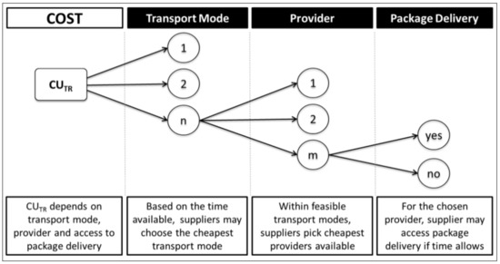
Figure 1.
Definition of transportation cost based on time available.
- “Transport-Mode”: being based on the time available for transportation, the supplier may choose to deliver via m different transport options (e.g., jet, truck, rail etc.), preferring the lowest-cost option that is able to deliver within the expected delivery date;
- “Provider”: since the preferred providers (tier 1) may not have assets available to accept last minute loads, the supplier has to move on to the next provider(s) n in order of preference (tier 2, 3, …) complete with increased costs, until the load is accepted;
- “Package Delivery” enables the reduction of costs by a certain value, as deliveries could be grouped, if the time available is sufficient to organize package delivery (the proper transportation lane and space have to be available)
In particular, let be the time available for delivery, that considers the standard time available for delivery (), plus the incremental time left from the APD, if any, after manufacturing ().
Since cheaper transportation options may be used when more time is available for delivery, suppliers may consider different transportation mode options, which we may call m (e.g., truck, rail, etc.), each of them with different providers, which we may call n, with the possibility of using package deliveries. All the options have different delivery times and costs. Let m be the transportation mode, e.g., jet, truck, rail, etc., and n the provider tier. As the decision tree shows, at any time t, if is higher than the minimum time threshold needed to book a cheaper transportation option, suppliers first choose the transportation mode (the first branch of the tree) and then check provider availability (the second branch of the tree), in order of cost preference (provider 1, 2, 3, …, n, with increasing rates), depending on the time available for delivery. Let Tm,n be the time to use the preferred provider in the chosen mode. For example, TRAIL,2 refers to the time needed to book the tier-2 rail provider. Finally, if the time left is sufficient (that is, the time left is higher than the time to access package delivery using a specific transport mode TPDm, suppliers check potential access to package delivery, that would imply a reduction of costs/discount of a value PDn (<1), as we could group our products and deliver them bundled with others, to leverage the same delivery (third branch of the tree).
In formulas, T&W benefits () can be calculated as in (6).
is the cost saving per unit per transportation choice, depending on the time available for delivery, with () and without () the APD program. For example, is the cost of the tier-2 rail provider.
As regards the benefits due to savings in Inventory Costs (IC), we can calculate the difference between IC under “standard” vs. APD conditions. The APD programs, in fact, increase supply chain visibility and thus the time available to allow an improved inventory management. In particular, in order to assess the IC benefits (), first we need to assess the inventory level change (ΔINV), starting from the current inventory level INV. This level will decrease by a certain value, depending on the bullwhip effect reduction (BW) expected as a consequence of the implementation of an APD program. BW can be calculated through literature [85] and/or by soliciting experts’ opinion, with a value that may range from 10% to 40%. In formula:
For the inventory unit cost (), we consider the working capital value, quantified on the basis of the weighted average cost of capital (WACC) and obsolescence costs (IDE, inventory depreciation expenses) associated with the rate of obsolescence (as a yearly turnover of codes, i.e., a percentage that depends on the specific business), and the regular price P. In formula:
According to the developed model, the supplier’s profit, i.e., the actual value of the APD program for the supplier, can be determined as the sum of the net benefits provided by the APD program at each time t during the time horizon T (as in Equation (9)).
where and is the periodic discount rate calculated from the annual rate depending on the number of periods (p) considered in the year. According to the supplier’s profit created by the APD, the supplier will decide whether or not to launch an APD program with the downstream retailer at the beginning of the commercial year.
From the retailer’s standpoint, the retailer’s profit from using an APD can be assessed as the discount received under the APD minus the inventory cost on account of the units bought under the APD program and that remain unsold at the end of the selling season.
where ωt is the dummy variable describing supplier behavior (i.e., ωt = 1 if the supplier engages in the program, 0 otherwise), I is the fraction of the unsold units at the end of the selling season, and is the inventory cost for the retailer.
Once the simulation model is in place we proceed to verify and validate the conceptual model to ensure that it was developed in accordance with the problem statement.
To verify a simulation model, it is necessary to establish whether the computer implementation of the conceptual model is correct. @Risk, the risk analysis software using Monte Carlo simulation for MS Excel, was used to build the simulation model. Given the complexity of the model, we compared the output of parts of the model with manually calculated solutions to ensure that the simulation logic worked as desired. We also proceeded to test run the simulation with no probabilistic elements to identify any errors in coding or logic.
After the simulation was run, the results were also validated. Model validation is the process of ensuring that the simulation accurately portrays the system under investigation [86]. Beyond mere face validity, which was established by perusing the flowchart, we validated the model by applying it to a real supply chain and reviewing the model and its outputs in a structured walk-though with company management. The next section describes the model applications and discusses the related results.
4. A Numerical Application: The Case of a Fortune 100 Company
In this section, we apply the developed model to the real case of a leading Fortune 100 company in the Fast Mover Consumer Goods (FMCG) industry. It is a large multinational company with a single production facility and demand from multiple retailers across different markets. For the sake of the study, we consider a single product and the product demand of the biggest retailer (for that product) so as to model this SC as a two-stage one, with one supplier and one retailer.
4.1. The Model’s Inputs
The model is applied based on data adapted from a full-scale case study of a production facility in EMEA (a region including Europe, Middle East and Africa), with realistic market values and operational conditions, adjusted by a specific coefficient for reasons of confidentiality. We consider a time horizon of one year, with twelve (monthly) windows where the supplier can exercise the option to offer discounted products to retailers that purchase in advance. For logistics, we consider the possibility of using two transportation mode options (m = rail or truck) respectively with two providers (n = 1 or 2).
The problem data consist of both estimates from expert interviews and historical data, when available. In particular, for expert interviews, data were gathered through three Sales Managers, four Supply Chain and Logistic Managers, and two Plant Production Managers.
Variables are grouped into deterministic and stochastic data (illustrated in Table 1 and Table 2, respectively). The following assumptions were used for the stochastic data:

Table 1.
Deterministic Variables.
Table 2.
Deterministic Variables.
- We assume that product demand (Dt) will vary stochastically in time following a Geometric Brownian Motion (GBM) [87,88]. This model is based on the assumption that demand can never be negative. It is mathematically described as in (11):
Historical data for products of the same brand over the last three years were used to estimate the growth rate μD, and volatility σD.
- We assume that the portion of demand that the retailer will allocate to APD (Qt) will vary stochastically in time, depending on both the historical behavior of the retailer and the APD discount, as described in (12).
In particular, we model the minimum quantity bought under the APD as a Mean Reverting (MR) process, according to the expectation of interviewed experts. Based on historical data, which reveal that there is a minimum constant demand across the different periods, the experts forecast that, in all likelihood, the retailer will devote a minimum portion of the total demand—on average—to the APD (without incurring additional costs). In other words, the portion of demand that the retailer will allocate to APD Qt fluctuates around a certain “equilibrium level” that is estimated with this minimum stable portion of the demand expressed periodically by the retailer, as described mathematically in (13).
where is the long run mean (mean reversion level), σ the volatility, α the mean reversion rate, and dWt is a Brownian motion (so ). All these parameters were estimated by considering the historical data for demand.
As suggested by experts, such minimum quantity should be adjusted by an additional portion β linked to the APD discount (the higher the discount offered, the higher the likelihood customers will allocate more volume) and by a random coefficient θt that simulates the real engagement of the retailer.
- For crashing and tardiness times (, , as statistically relevant historical data are not available, we reached out to production experts from the plant. Since experts generally do not know these values with any certainty, they usually express them as three-point estimates (reflecting the best/worst/most likely scenarios for the considered variable. Experts’ opinions expressed as three point-estimates are usually modeled as non-parametric probability distributions rather than parametric distributions where shape and range are determined by one or more distribution-specific parameters (which is more difficult to assess) [89]. One of the most commonly used probability distributions is the BetaPert distribution, which, strictly speaking, is a parametric distribution (since it derives from Beta) adapted to be able to estimate only min, max and expected values. Compared to triangular distributions, a BetaPert may be closer to a bell-shaped distribution, to give more importance to the central value rather than the extremes.
- For bullwhip effect reduction (BW, that will have a direct impact on inventory reduction), the literature generally considers a range between 10% and 40% [85]. Therefore, as statistically relevant historical data are not available, we reached out to supply chain experts to check what the expected value range in this case might be. The experts returned a range between 15% and 25%, with the same probability between the extremes. This suggests the use of a Uniform distribution. For perspective, the difference in the upper bound of the distribution (estimated rather than literature) arises from the fact that the experts considered 40% as high considering also the high service levels required in the industry.
- The fraction of the unsold units at the end of selling season I is a uniformly distributed variable, ranging between 0% (i.e., all the quantity ordered under the APD program has been sold) and a maximum quantity that, as suggested by the experts, is linked to the time of advanced orders TAPD (the higher the pre-order time, the greater the likelihood that retailers will have a higher level of unsold units at the end of the selling season compared with the simpler contract).
As for the additional costs generated by the APD compared with simpler contracts (Co), as suggested by the interviewed Managers, they basically consist in the system investment costs to integrate APD into the pricing and lead time structure in the ERP (Enterprise Resources Planning) system, and the cost of the expert manager who handles the contract.
A Monte Carlo simulation was run using the @Risk software. The discount rate in the Monte Carlo simulation is generally a risk-free rate [90], since the risk is already included in the cash flows that depend on the randomly chosen values of the input parameters.
4.2. Results
Figure 2 plots the probability distributions of the supplier’s and the retailer’s profits under the APD program derived for this first setting (K = 1.5% and = 10 days) after 10,000 computer iterations.
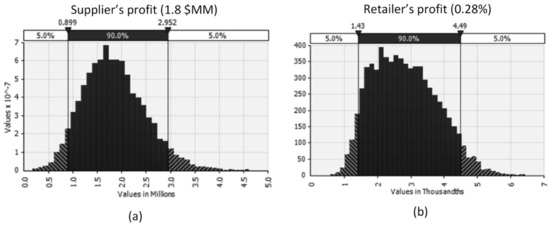
Figure 2.
Probability distributions of the supplier’s profit (a) and the retailer’s profit (b) for the first setting.
For this first setting, the supplier’s profit ΠS ranges within the interval [0.2–4.6] $MM with a probability of 90% (the 5th percentile is 0.9 $MM), a mean 1.8 MM$, and a median equal to 1.79 $MM.
The retailer’s profit ΠR expressed as a percentage of the retailer’s spend ranges within the interval [0.060–0.596] %, with a probability of 90% (the 5th percentile is 0.1), a mean 0.28%, and a median equal to 0.27%.
As a first result, we found that the chain partners obtain higher profits than when the APD contract is absent. This means that in this setting the APD contract creates value for both the actors. In particular, the additional costs of APD contracts for the supplier are fully covered, and even outweighed by their benefits; at the same time, the retailer receives price discount savings from advanced purchases without any risk of loss in placing an advanced order. Hence, since both the profits are calculated as the differential value created by the APD contract compared with the base case without the APD, the sum of the SC actors’ profits (i.e., SC profit ΠSC) is the measure of SC efficiency pursued by channel coordination achieved through the APD program.
These considerations suggest that the APD may be a very attractive contract. Given a supplier and a retailer, it may coordinate the supply chain and divide the resulting profits for any reasonable function that depends on the retailer’s purchase quantity, price, discount, and all the other parameters of the contract.
With so much going for it, one might argue that in such conditions (i.e., positive profits for both chain partners), the APD should be ubiquitous. Actually, another important element that should be observed, beyond the profits, is the number of activations of the APD program during the time horizon of the program, namely the number of times the supplier exercises the option. Figure 3 plots the probability distribution of the number of activations of the APD program during the time horizon of the program for this first setting, within the interval (4–12) with a probability of 90% (the 5th percentile is 8), a mean of 10.3, and the median equal to 11.

Figure 3.
Probability distribution of number of APD activations for the first setting.
The number of activations expected throughout the time horizon of the validity of the program Ω is an important indicator because when it is low, the supplier will probably avoid promoting the program with the retailer at the beginning of the commercial year (irrespective of the chain partners’ profit values), to avoid systematically denying its applicability, as the expected benefits are lower than the relative costs in year t.
4.3. Sensitivity Analysis
In order to analyze how the contract parameters can be modified so as to share the profit and risks more evenly along the chain (a win–win condition for the chain partners), while guaranteeing channel coordination, we ran a sensitivity analysis on the APD contract terms, namely the APD discount K and the APD time TAPD.
In particular, Figure 4 shows the results of sensitivity on the APD discount.
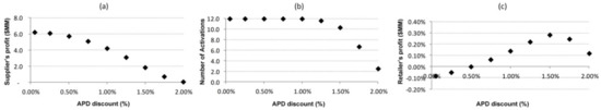
Figure 4.
Sensitivity charts with APD discount: Supplier’s profit (a), Number of Activations (b) and Retailer’s profit (c).
As Figure 4a illustrates, when the APD discount increases, the supplier’s profit decreases in an almost linear fashion. The retailer’s profit is concave (Figure 4c). It starts from negative values, thus implying that the low discount does not adequately compensate for the retailer’s risk in placing an advanced order. It becomes positive when K = 0.5%, and then reaches the highest value for the basic setting (K = 1.5%). This finding has two main implications. Firstly, any time the supplier offers a discount, the retailer receives price discount savings from advanced purchases, but it is very risky for the retailer to place an advanced order (since (s)he may also incur a loss). This supports the importance of quantifying the benefits associated with such contracts, and setting the contract parameters in order to ensure a win-win condition for both chain partners. Secondly, this concave function is not intuitive, since one would expect that the higher the APD discount, the higher the retailer profit. We argue that this is mainly linked to the exponential decrease in the number of activations (i.e., the number of times the supplier exercises the option) (see Figure 4b). When the APD discount increases, the supplier has less of an incentive to offer the discount, producing fewer savings for the retailer.
As a further result of sensitivity on the APD discount, we analyse the risk profile of both the chain partners (Figure 5), defined as the probability that the net profit generated by the APD contract is negative.
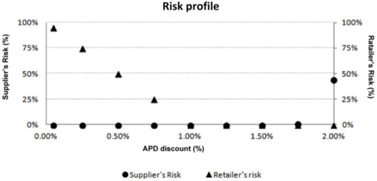
Figure 5.
Sensitivity charts with APD discount: Supplier’s and Retailer’s risk profile.
As illustrated in Figure 5, the supplier’s risk increases when the discount increases, while the retailer’s risk decreases when the discount increases. In light of this finding, we can infer that the contract seems fairly able to allocate risk when the discount offered ranges between [1–1.75%]. This implies that the APD contract is able to ensure SC coordination, given a proper setting for the APD discount.
Figure 6 shows the analysis results from a time-sensitivity standpoint (TAPD).
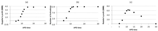
Figure 6.
Sensitivity charts with APD time: Supplier’s profit (a), Number of Activations (b) and Retailer’s profit (c).
From Figure 6a we can observe that the supplier’s profit is low when the values of TAPD are low (it may also be negative for lower values of APD time, meaning that in such cases, the benefits may not outweigh the cost of adopting APD contracts due to the low number of activations). Then, it sharply increases rapidly from a certain value of APD time, and follows an asymptotic trend for higher values of APD time. On the other hand, the retailer’s profit is concave (Figure 6c). The profit increases up to a certain value, after which it decreases until it becomes 0 for high values of APD time. We argue that the choice of advancing the order too much may erode the retailer’s profit, making the contract unsuccessful for this chain partner. Therefore, the APD time has to be set properly in order to ensure channel coordination and win-win conditions. Finally, we analyse the risk profile for both chain partners when the APD time varies. As Figure 7 shows, the supplier’s risk decreases when the APD time increases, while the retailer’s risk increases when the APD time increases.
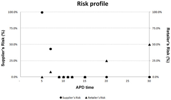
Figure 7.
Sensitivity charts with APD time: Supplier’s and Retailer’s risk profile.
5. Conclusions
This paper focuses on the issue of SCF coordination under decentralized control, where each SC actor makes decisions by optimizing his/her own objective. A supply contract, namely the Advance Purchase Discount (APD) program, was modelled as a contract option to coordinate the capital flow and improve the efficiency of a two-stage SC with stochastic customer demand.
Our first research contribution is to fill the gap in the existing literature, which is lacking in studies exploring how advanced information about customer needs obtained through the APD contract can be exploited to coordinate a SC under decentralized control. Furthermore, in order to take into account the flexible behavior of the upstream firm and to decide whether to provide a discount for an advance purchase at its own discretion, we modeled an APD as an option contract, thus including the value created by the firm’s flexibility to engage in the program only if it will be profitable.
After applying the developed model to the real case of a large multinational company (Fortune 100) in the Fast-Moving Consumer Goods (FMCG) industry, we gained managerial insights as to when such programs should be instituted.
Firstly, under an APD, the partners in the chain may obtain profits higher than when there is no APD contract; hence, the APD may ensure a win-win condition. The extent of SC efficiency pursued by the channel coordination achieved through the APD program is measured by the sum of the SC actors’ profits. These considerations support the hypothesis that the APD may constitute a very attractive contract. In the case of a single supplier and retailer, it coordinates the supply chain and divides the resulting profits in terms of any reasonable function that depends on the retailer’s purchase quantity, price, discount, and all the other parameters of the contract.
With so much going for it, one might argue that the APD should be ubiquitous. However, even when the APD contract creates profits for both the chain partners, we show that the number of activations of the APD program during the time horizon of the validity of the program is an important element to take into consideration, not only the profits. The supplier has to carefully decide whether to promote the APD program with the retailer at the beginning of the commercial year. Deciding to promote the program at the beginning of the year and then denying its applicability to the retailer almost systematically as the expected benefits are lower than the related costs effectively means eroding the advantage created by the program itself.
By promoting APD only when it is activated a certain number of times to deliver the expected/negotiated value, the APD may ensure the channel coordination and the win-win condition.
In addition, a sensitivity analysis revealed that the discount-time binomial for the APD has to be carefully assessed in order to ensure that this kind of contract succeeds as a coordination mechanism. We found that the APD contract shifts some risk from the supplier to the retailer, and the amount of transferred risk depends on the discount-time binomial for the APD. When the APD discount is too low or the APD time is too high, the risk is unbalanced towards the retailer. When the APD discount is too high or the APD time is too low, on the other hand, the contract loses its value for the supplier. Therefore, since the APD value cannot be predicted by simply looking at the input data, it is crucial to properly estimate the benefits associated with such contracts. Also, cooperation among the SC actors during the contract design phase (i.e., contract parameter definition) would make adopting the APD a strategic way to maximize the SC profits (win-win condition), while guaranteeing channel coordination.
This work, however, is not without limitations. Firstly, we considered a two-stage SC with only two actors, but actually, multistage supply chains better describe real SCs. Further, considering only one retailer did not allow us to embed the effect of competition among multiple retailers. Further research will be devoted to investigating all these limitations.
Author Contributions
R.P., N.C. and D.T. conceived the study; R.P. conducted the literature review, R.P. and D.T. developed the model, and designed the experiments; D.T. performed the experiments; R.P., N.C. and D.T. analyzed the data and results; and R.P., N.C. and D.T. edited the final version of the paper. All authors have read and agreed to the published version of the manuscript.
Funding
This research received no external funding.
Acknowledgments
The authors would like to thank the leading Fortune 100 multinational company in the Fast Mover Consumer Goods (FMCG) industry participating in this research for its support in the collection of field data and model verification.
Conflicts of Interest
The authors declare no conflict of interest.
References
- Christopher, M. Logistics and Supply Chain Management; Pitman Publishing: London, UK, 1992. [Google Scholar]
- Tsay, A.A.; Nahmias, S.; Agrawal, N. Modeling supply chain contracts: A review. In Quantitative Models for Supply Chain Management; Tayur, S., Ganeshan, R., Magazine, M., Eds.; Kluwer Academic Publisher: Norwell, MA, USA, 1999; pp. 299–336. [Google Scholar]
- Giannoccaro, I.; Pontrandolfo, P. Supply chain coordination by revenue sharing contracts. Int. J. Prod. Econ. 2004, 89, 131–139. [Google Scholar] [CrossRef]
- Schneeweiss, C. Distributed decision making in supply chain management. Int. J. Prod. Econ. 2003, 84, 71–83. [Google Scholar] [CrossRef]
- Whang, S. Coordination in operations: A taxonomy. J. Oper. Manag. 1995, 12, 413–422. [Google Scholar] [CrossRef]
- Lee, H.L.; Billington, C. The evolution of supply chain management models and practices at Hewlett-Packard. Interfaces 1995, 25, 42–63. [Google Scholar] [CrossRef]
- Lambert, D.M.; Cooper, M.C.; Pagh, J.D. Supply chain management: Implementation issues and research opportunities. Int. J. Logist. Manag. 1998, 9, 1–12. [Google Scholar] [CrossRef]
- Cachon, G.P.; Zipkin, P.H. Competitive and cooperative inventory policies in a two-stage supply chain. Manag. Sci. 1999, 45, 936–953. [Google Scholar] [CrossRef]
- Frohlich, M.T.; Westbrook, R. Arcs of integration: An international study of supply chain strategies. J. Oper. Manag. 2001, 19, 185–210. [Google Scholar] [CrossRef]
- De Kok, T.; Janssen, F.; van Doremalen, J.; van Wachem, E.; Clerkx, M.; Peeters, W. Electronics synchronizes its supply chain to end the bull whip effect. Interfaces 2005, 35, 37–48. [Google Scholar] [CrossRef]
- Tang, S.Y.; Kouvelis, P. Pay-Back-Revenue-Sharing Contract in Coordinating Supply Chains with Random Yield. Prod. Oper. Manag. 2014, 23, 2089–2102. [Google Scholar] [CrossRef]
- Saudi, M.H.M.; Juniati, S.; Kozicka, K.; Razimi, M.S.A. Influence of lean practices on supply chain performance. Pol. J. Manag. Stud. 2019, 19, 353–363. [Google Scholar] [CrossRef]
- Saudi, M.H.M.; Sinaga, H.O.; Roespinoedji, D.S. The role of tax education in supply chain management a case of Indonesian supply chain companies. Pol. J. Manag. Stud. 2018, 18, 284–299. [Google Scholar] [CrossRef]
- Kot, S.; Goldbach, I.R.; Ślusarczyk, B. Supply chain management in SMEs-Polish and Romanian approach. Econ. Sociol. 2018, 11, 142–156. [Google Scholar] [CrossRef]
- Kot, S.; Haque, A.; Baloch, A. Supply Chain Management in SMEs: Global Perspective. Montenegrin J. Econ. 2020, 16, 87–104. [Google Scholar] [CrossRef]
- Narayanan, V.G.; Raman, A. Aligning incentives in supply chains. Harvard Bus. Rev. 2004, 82, 94–103. [Google Scholar]
- Asian, S.; Nie, X. Coordination in supply chains with uncertain demand and disruption risks: Existence, analysis, and insights. IEEE Trans. Syst. Man Cybern. Syst. 2014, 44, 1139–1154. [Google Scholar] [CrossRef]
- Cachon, G.P. Supply Chain Coordination with Contracts. In Handbooks in Operations Research and Management Science: Supply Chain Management; Graves, S., de Kok, T., Eds.; Elsevier: Amsterdam, The Netherlands, 2003. [Google Scholar]
- Choi, T.M. Supply chain systems coordination with multiple risk sensitive retail buyers. IEEE Trans. Syst. Man Cybern. Syst. 2016, 46, 636–645. [Google Scholar] [CrossRef]
- Kouvelis, P.; Zhao, W. Supply chain contract design under financial constraints and bankruptcy costs. Manag. Sci. 2015, 62, 2341–2357. [Google Scholar] [CrossRef]
- Chakuu, S.; Masi, D.; Godsell, J. Exploring the relationship between mechanisms, actors and instruments in supply chain finance: A systematic literature review. Int. J. Prod. Econ. 2019, 216, 35–53. [Google Scholar] [CrossRef]
- Gelsomino, L.U.C.A.; Mangiaracina, R.; Perego, A.; Tumino, A. Supply chain finance: A literature review. Int. J. Phys. Distrib. Logist. Manag. 2016, 46. [Google Scholar] [CrossRef]
- Hofmann, E.; Belin, O. Supply Chain Finance Solutions; Springer: Berlin/Heidelberg, Germany, 2011; pp. 644–645. [Google Scholar]
- Wang, Z.; Wang, Q.; Lai, Y.; Liang, C. Drivers and outcomes of supply chain finance adoption: An empirical investigation in China. Int. J. Prod. Econ. 2020, 220, 107453. [Google Scholar] [CrossRef]
- Gomm, M.L. Supply chain finance: Applying finance theory to supply chain management to enhance finance in supply chains. Int. J. Logist. Res. Appl. 2010, 13, 133–142. [Google Scholar] [CrossRef]
- Xu, X.; Chen, X.; Jia, F.; Brown, S.; Gong, Y.; Xu, Y. Supply chain finance: A systematic literature review and bibliometric analysis. Int. J. Prod. Econ. 2018, 204, 160–173. [Google Scholar] [CrossRef]
- Lin, Q.; Su, X.; Peng, Y. Supply chain coordination in confirming warehouse financing. Comput. Ind. Eng. 2018, 118, 104–111. [Google Scholar] [CrossRef]
- Shi, J.; Du, Q.; Lin, F.; Li, Y.; Bai, L.; Fung, R.Y.; Lai, K.K. Coordinating the supply chain finance system with buyback contract: A capital-constrained newsvendor problem. Comput. Ind. Eng. 2020, 146, 106587. [Google Scholar] [CrossRef]
- Pellegrino, R.; Costantino, N.; Tauro, D. Supply Chain Finance: A supply chain-oriented perspective to mitigate commodity risk and pricing volatility. J. Purch. Supply Manag. 2019, 25, 118–133. [Google Scholar] [CrossRef]
- Eppen, G.D.; Iyer, A.V. Backup agreements in fashion buying—The value of upstream flexibility. Manag. Sci. 1997, 43, 1469–1484. [Google Scholar] [CrossRef]
- Emmons, H.; Gilbert, S.M. Note: The role of returns policies in pricing and inventory decisions for catalogue goods. Manag. Sci. 1998, 44, 276–283. [Google Scholar] [CrossRef]
- Lee, H.L.; Whang, S. Decentralized multi-echelon supply chains: Incentives and information. Manag. Sci. 1999, 45, 633–640. [Google Scholar] [CrossRef]
- Cachon, G.P.; Lariviere, M.A. Supply chain coordination with revenue sharing contracts: Strength and limitations. Manag. Sci. 2005, 51, 30–44. [Google Scholar] [CrossRef]
- Cachon, G.; Lariviere, M.A. Capacity choice and allocation: Strategic behavior and supply chain performance. Manag. Sci. 1999, 45, 1091–1108. [Google Scholar] [CrossRef]
- Weng, Z.K. Channel coordination and quantity discounts. Manag. Sci. 1995, 41, 1509–1522. [Google Scholar] [CrossRef]
- Tang, C.S.; Rajaram, K.; Alptekinoğlu, A.; Ou, J. The benefits of advance booking discount programs: Model and analysis. Manag. Sci. 2004, 50, 465–478. [Google Scholar] [CrossRef]
- Bernstein, F.; DeCroix, G.A. Advance demand information in a multiproduct system. Manuf. Serv. Oper. Manag. 2014, 17, 52–65. [Google Scholar] [CrossRef]
- Cachon, G.P. The Allocation of Inventory Risk in a Supply Chain: Push, Pull, and Advance-Purchase Discount Contracts. Manag. Sci. 2004, 50, 222–238. [Google Scholar] [CrossRef]
- Cho, S.H.; Tang, C.S. Advance selling in a supply chain under uncertain supply and demand. Manuf. Serv. Oper. Manag. 2013, 15, 305–319. [Google Scholar] [CrossRef]
- Li, C.; Zhang, F. Advance demand information, price discrimination, and preorder strategies. Manuf. Serv. Oper. Manag. 2013, 15, 57–71. [Google Scholar] [CrossRef]
- Nasiry, J.; Popescu, I. Advance selling when consumers regret. Manag. Sci. 2012, 58, 1160–1177. [Google Scholar] [CrossRef]
- Yu, M.; Kapuscinski, R.; Ahn, H.S. Advance selling: Effects of interdependent consumer valuations and seller’s capacity. Manag. Sci. 2015, 61, 2100–2117. [Google Scholar] [CrossRef]
- Gilbert, S.M.; Ballou, R.H. Supply chain benefits from advanced customer commitments. J. Oper. Manag. 1999, 18, 61–73. [Google Scholar] [CrossRef]
- Tang, W.; Girotra, K. Synchronizing Global Supply Chains: Advance Purchase Discounts. Working Paper. 2010. Available online: http://www.insead.edu/facultyresearch/research/doc.cfm?did=43578 (accessed on 3 December 2013).
- McCardle, K.; Rajaram, K.; Tang, C. Advance Booking Discount Programs under Retail Competition. Manag. Sci. 2004, 50, 701–708. [Google Scholar] [CrossRef]
- Xie, J.; Shugan, S. Electronic tickets, smart cards, and online prepayments: When and how to advance sell. Market. Sci. 2001, 20, 219–243. [Google Scholar] [CrossRef]
- Dana, J., Jr. Advance-Purchase Discounts and Price Discrimination in Competitive Markets. J. Political Econ. 1998, 106, 395–422. [Google Scholar] [CrossRef]
- Gundepudi, P.; Rudi, N.; Seidmann, A. Forward vs. spot buying of information goods on Web: Analysing the consumer decision process. J. Manag. Inf. Syst. 2001, 18, 107–131. [Google Scholar] [CrossRef]
- Akan, M.; Ata, B.; Dana, J. Revenue Management by Sequential Screening; Working Paper; Northwestern University: Evanston, IL, USA, 2009. [Google Scholar]
- Bellantuono, N.; Giannoccaro, I.; Pontrandolfo, P.; Tang, C. The implications of joint adoption of revenue sharing and advance booking discount programs. Int. J. Prod. Econ. 2009, 121, 383–394. [Google Scholar] [CrossRef]
- Donohue, K. Efficient supply contracts for fashion goods with forecast updating and two production modes. Manag. Sci. 2000, 46, 1397–1411. [Google Scholar] [CrossRef]
- Ozer, O.; Uncu, O.; Wei, W. Selling to the newsvendor with a forecast update. Eur. J. Oper. Res. 2007, 182, 1150–1176. [Google Scholar] [CrossRef]
- Kogut, B.; Kulatilaka, N. Option thinking and platform investment: Investing in opportunity. Calif. Manag. Rev. 1994, 36, 52–71. [Google Scholar] [CrossRef]
- Boute, R.; Demeulemeester, E.; Herroelen, W. A real options approach to project management. Int. J. Prod. Res. 2004, 42, 1715–1725. [Google Scholar] [CrossRef]
- Olafsson, S. Making decisions under uncertainty—Implications for high technology investments. BT Technol. J. 2003, 21, 170–183. [Google Scholar] [CrossRef]
- Luehrman, T.A. Investment Opportunities as Real Options: Getting Started on the Numbers; Harvard Business Review: Boston, MA, USA, 1998. [Google Scholar]
- Trigeorgis, L. Real Options; The MIT Press: Cambridge, MA, USA, 1996. [Google Scholar]
- Wang, X.; Liu, L. Coordination in a retailer-led supply chain through option contract. Int. J. Prod. Econ. 2007, 110, 115–127. [Google Scholar] [CrossRef]
- Newbery, D. Competition, contracts, and entry in the electricity spot market. RAND J. Econ. 1998, 29, 726–749. [Google Scholar] [CrossRef]
- Spinler, S.; Huchzermeier, A.; Kleindorfer, P. Options on capacity: Applications to e-transport platforms. In Logistics Management; Sebastian, H.J., Grünert, T., Eds.; Teubner: Stuttgart, Germany, 2001; pp. 305–315. [Google Scholar]
- Spinler, S.; Huchzermeier, A.; Kleindorfer, P. An options approach to enhance economic efficiency in a dyadic supply chain. In Cost Management in Supply Chains; Stefan, S., Maria, G., Eds.; Physica: Heidelberg, Germany, 2002; pp. 350–360. [Google Scholar]
- Wu, D.; Kleindorfer, P.; Zhang, J. Optimal bidding and contracting strategies for capital-intensive goods. Eur. J. Oper. Res. 2002, 137, 657–676. [Google Scholar] [CrossRef]
- Barnes-Schuster, D.; Bassok, Y.; Anupindi, R. Coordination and flexibility in supply contracts with options. Manuf. Serv. Oper. Manag. 2002, 4, 171–207. [Google Scholar] [CrossRef]
- Milner, J.M.; Rosenblatt, M.J. Flexible supply contracts for short life-cycle goods: The buyer’s perspective. Nav. Res. Logist. 2002, 49, 25–45. [Google Scholar] [CrossRef]
- Wang, Q.Z.; Tsao, D.B. Supply contract with bidirectional options: The buyer’s perspective. Int. J. Prod. Econ. 2006, 101, 30–52. [Google Scholar] [CrossRef]
- Cheng, F.; Ettl, M.; Lin, G.Y.; Schwarz, M.; Yao, D.D. Flexible Supply Contracts via Options; Working Paper; IBM T.J. Watson Research Center: Yorktown Heights, NY, USA, 2003. [Google Scholar]
- Cachon, G.; Lariviere, M.A. Contracting to assure supply: How to share demand forecasts in a supply chain. Manag. Sci. 2001, 47, 629–646. [Google Scholar] [CrossRef]
- Costantino, N.; Pellegrino, R. Choosing between single and multiple sourcing based on supplier default risk: A real options approach. J. Purch. Supply Manag. 2010, 16, 27–40. [Google Scholar] [CrossRef]
- Black, F.; Scholes, M. The pricing of options and corporate liabilities. J. Political Econ. 1973, 81, 637–654. [Google Scholar] [CrossRef]
- Merton, R.C. The Theory of Rational Option Pricing. Bell J. Econ. Manag. Sci. 1973, 4, 141–183. [Google Scholar] [CrossRef]
- Boyle, P.P. Options: A Monte Carlo Approach. J. Financ. Econ. 1977, 4, 323–338. [Google Scholar] [CrossRef]
- Cox, J.C.; Ross, S.A.; Rubinstein, M. Option pricing: A simplified approach. J. Financ. Econ. 1979, 7, 229–263. [Google Scholar] [CrossRef]
- Longstaff, F.A.; Schwartz, E.S. Valuing American Options by Simulation: A Simple Least-Squares Approach. Rev. Financ. Stud. 2001, 14, 113–147. [Google Scholar] [CrossRef]
- De Neufville, R.; Scholtes, S.; Wang, T. Real Options by Spreadsheet: Parking Garage Case Example. J. Infrastruct. Syst. 2006, 12, 107–111. [Google Scholar] [CrossRef]
- Lander, D.M.; Pinches, G.E. Challenges to the Practical Implementation of Modelling and Valuing Real Options. Q. Rev. Econ. Financ. 1998, 38, 537–567. [Google Scholar] [CrossRef]
- Evers, P.T.; Wan, X. Systems analysis using simulation. J. Bus. Logist. 2012, 33, 80–89. [Google Scholar] [CrossRef]
- Chang, Y.; Makatsoris, H. Supply chain modelling using simulation. Int. J. Simul. 2001, 2, 24–30. [Google Scholar]
- Goldsby, T.J.; Griffis, S.E.; Roath, A.S. Modeling lean, agile, and leagile supply chain strategies. J. Bus. Logist. 2006, 27, 57–80. [Google Scholar] [CrossRef]
- Wan, X.; Evers, P.T. Supply chain networks with multiple retailers: A test of the emerging theory on inventories, stockouts, and bullwhips. J. Bus. Logist. 2011, 32, 27–39. [Google Scholar] [CrossRef]
- Manuj, I.; Mentzer, J.T.; Bowers, M.R. Improving the rigor of discrete-event simulation in logistics and supply chain research. Int. J. Phys. Distrib. Logist. Manag. 2009, 39, 172–201. [Google Scholar] [CrossRef]
- Manuj, I.; Esper, T.L.; Stank, T.P. Supply chain risk management approaches under different conditions of risk. J. Bus. Logist. 2014, 35, 241–258. [Google Scholar] [CrossRef]
- Chiara, N.; Garvin, M.; Vecer, J. Valuing Simple Multiple-Exercise Real Options in Infrastructure Projects. ASCE J. Infrastruct. Syst. 2007, 13, 97–104. [Google Scholar] [CrossRef]
- Cakravastia, A.; Toha, I.S.; Nakamura, N. A two-stage model for the design of supply chain networks. Int. J. Prod. Econ. 2002, 80, 231–248. [Google Scholar] [CrossRef]
- Slotnick, S.A.; Sobel, M.J. Manufacturing lead-time rules: Customer retention versus tardiness costs. Eur. J. Oper. Res. 2005, 163, 825–856. [Google Scholar] [CrossRef]
- AMR Research. Beyond CPFR: Collaboration Comes of Age, The Report on Retail E-Business; AMR Research: Boston, MA, USA, 2001. [Google Scholar]
- Law, A.M. Simulation Modeling and Analysis; McGraw-Hill: New York, NY, USA, 2006. [Google Scholar]
- Benavides, D.L.; Duley, J.R.; Johnson, B.E. As good as it gets: Optimal Fab design and deployment. IEEE Trans. Semicond. Manuf. 1999, 12, 281–287. [Google Scholar] [CrossRef]
- Chou, Y.C.; Cheng, C.T.; Yang, F.C.; Liang, Y.Y. Evaluation of alternative capacity strategies in semiconductor manufacturing under uncertain demand and price scenarios. Int. J. Prod. Econ. 2007, 105, 591–606. [Google Scholar] [CrossRef]
- Vose, D. Quantitative Risk Analysis. A Guide to Monte Carlo Simulation Modelling; John Wiley & Sons: Hoboken, NJ, USA, 1996. [Google Scholar]
- Brealey, R.; Myers, S. Principles of Corporate Finance, 6th ed.; Irwin McGraw-Hill: Boston, MA, USA, 2000. [Google Scholar]


Publisher’s Note: MDPI stays neutral with regard to jurisdictional claims in published maps and institutional affiliations. |
© 2020 by the authors. Licensee MDPI, Basel, Switzerland. This article is an open access article distributed under the terms and conditions of the Creative Commons Attribution (CC BY) license (http://creativecommons.org/licenses/by/4.0/).