Abstract
Highways passing through cities cause additional pollution inside the city. However, most of the current studies are using ground-based monitoring technologies, which make it difficult to capture the dispersion patterns of pollutants near elevated highways or transportation interchanges. The purpose of this study is to discover short-term three-dimensional variations in traffic-related pollutants based on unmanned aerial vehicles. The monitoring locations are at suburban elevated highway and transportation interchanges. The monitoring parameters include the particle number concentration (PN), particle mass concentration (PM), and black carbon (BC). The vertical profiles showed that most air pollutants increased significantly with the height of the elevated highways. Compared with the ground level, PNs increased by 54%–248% and BC increased by 201%. The decline rate of particle concentrations decreased with the increase of height and remained stable after 120 m. Furthermore, the R2 heatmap for regressions between each altitude showed that the linear relationship between 0–120 m was higher than that of other altitudes. In horizontal profiles, PNs spread to 100 m and then began to decline, BC began to decay rapidly after 50 m, but PMs varied less. After crossing another highway, PNs increased by 69–289%, PMs by 7–28%, and BC by 101%. Furthermore, the formation of new particles was observed at both locations as PN3 increased with distance within 100 m from the highway. This paper fills in the void of three-dimensional in situ monitoring near elevated highways, and can help develop and refine a three-dimensional traffic-related air pollution dispersion model and assess the impacts of transportation facilities on the urban environment.
1. Introduction
Air pollution is a major environmental challenge in urban areas [1]. Ambient particulate matter pollution will increase mortality and morbidity and has become one of the leading four risk factors contributing to death in China [2,3,4]. In highly populated urban areas, traffic is a major local source of ambient air pollution [5]. Congested traffic conditions also exacerbate air pollutant emissions from vehicles in highly populated cities, especially since many of these vehicles move around continuously looking for parking spaces [6]. The main emissions of vehicles are ultrafine particles (UFPs) with an aerodynamic diameter of 0.25 to 2.5 μm. The emissions of traffic-related air pollutants are close to the human respiratory zone and seriously threaten human health. Furthermore, the size of the particles in the ambient air affects the amount of particles inhaled by humans and the distribution of these particles in the human body [7]. Fine fractions of particles related to road traffic emissions will cause adverse health effects [8]. Besides, black carbon (BC) is also a typical traffic-related pollutant and may have short- or long-term effects on human health [9,10]. Therefore, this study mainly investigates the number and mass concentration of 0.3–10 μm particles and the mass concentration of BC below 880 nm.
UFPs and other vehicle emissions are higher near highways but drop to the background within a few hundred meters [11]. The factors affecting the variation gradients include traffic conditions, temperature, relative humidity, topography, wind direction and speed, atmospheric stability, and mixing layer height [12,13]. UFP is very light, so it is often considered to be consistent with the diffusion characteristics of gaseous pollutants. At present, there are many methods to study the diffusion of roadside pollutants, including the vehicle-based mobile platform, fixed monitoring stations, and portable devices. Vehicle-based mobile platforms are usually equipped with on-board high time resolution air monitors and drive on the road at a very low speed to measure traffic-related pollutants. The measurements based on the mobile monitor platform are mainly taken on urban roads to investigate the attenuation gradients on the ground and the effect of urban street canyons [14]. The highest pollutant concentrations were observed within 0–50 m near the road [15,16] using the mobile platform, but the distance–decay gradients varied with traffic and meteorology. However, vehicle-based mobile platforms have many limitations, such as self-sampling and abnormal high values while stopped at traffic lights and stop signs. In addition, they are confined to the ground level and the road, which makes it impossible to obtain measurement data above the ground and in off-road areas. The fixed monitoring stations near the road are usually used for long-term observations and mainly to characterize temporal changes at one site or to compare different sites. A study monitored at 150 m away from an urban road [17] showed that roadway traffic contributes only 12–17% of the total PM2.5 roadside concentration. Concentrations of UFP, as well as other primary vehicular emissions, were elevated during traffic rush hours [18], reflecting ultrafine direct exhaust emissions. Another study [19] set two devices 1m away from a bus stop and 10 m away from the highway, and the result indicated that the particle number concentrations (PN) between 0.5 and 1 μm near the highway were higher than those at the bus stop. The fixed monitoring devices are deployed at fixed intervals away from the road to obtain attenuation information [20]. However, the mobility of this method is insufficient, and most devices are limited to the ground and to mobile monitoring. Furthermore, it is expensive to set up the fixed monitoring stations. Some studies use portable devices to measure the pollutants while walking or cycling [21,22], for pedestrian pollution exposure assessment and street canyon research. However, walking measurement is more susceptible to human influence such as breathing and resuspension of particles during walking, thereby reducing the accuracy of the measurement. At the same time, it is affected by the walking speed of the person, and the range of measurement is smaller than that of the vehicle-based mobile platform. Therefore, in order to develop a three-dimensional knowledge of the pollutants in the air, test the location effects of three-dimensional patterns, and provide data to develop and validate the roadside dispersion model, a monitoring method with good mobility and no self-generated pollution is needed, such as unmanned aerial vehicle (UAV) based monitoring. Battery-powered multirotor UAVs are characterized by high efficiency, good mobility, and the lack of emissions while flying. With portable devices appropriately installed on the UAV, it is maneuverable and can collect air quality data in areas where conventional methods are difficult to reach [23]. Based on the UAV platform, the pollution maps can be constructed and the high concentration hotspots can be discovered [24]. It can find the most polluted areas with a higher coverage within the time bounds defined by the UAV flight time [25,26]. UAVs can offer high-resolution spatiotemporal sampling, which is not possible or feasible with manned aircrafts [27]. The three-dimensional monitoring of the air quality data can help improve the performance and accuracy of the model and simulation.
Although some published studies have made important contributions to our understanding of the variations of air pollutants near the highway, the knowledge of three-dimensional air quality data above the ground is still missing. At present, studies on air pollutant variations near the highway are mostly confined to the ground, and the results show that 100 m away from the road, the concentrations decrease to background concentrations [28]. However, the investigation of whether the elevated highway has the same dispersion law above the ground is still lacking. Measuring the variations in pollutant gradients in close proximity to a highway can help develop three-dimensional patterns of the pollutants in the air, test the location effects of three-dimensional patterns, and provide data to develop and validate the roadside dispersion model. To fill the void of three-dimensional in situ monitoring of roadside air pollution, this paper investigates the variation of air pollutants near elevated highways with different road configurations for one of the main urban pollutants, particulate matter, by measuring three parameters: PN, particle mass concentration (PM), and BC.
2. Materials and Methods
2.1. Study Area Description
The experimental site is located in Dezhou, northwest of Shandong Province, China. There are 19 expressways in Dezhou, including the Beijing–Shanghai Expressway (G2), the Beijing–Taiwan Expressway (G3), etc. Until the end of 2018, there were a total of 4485.38 km of highways in Dezhou (excluding village roads, Shandong Provincial Bureau of Statistics, http://www.stats-sd.gov.cn/). The highway selected for the experiment is the G3 in eastern Dezhou, which overlaps with the G2 while passing through Dezhou. There are two lanes in each direction with a speed limit of 100–120 km/h, and the average daily traffic volume is 717–1317 vehicles/hour. In order to study the dispersion of pollutants above the ground near the elevated highways under different road configurations, the two selected locations were Laojianhe, at the south of Dezhou, and Shuniu, at the north of Dezhou (Figure 1). Laojianhe is located in the suburban area of the city, surrounded by a small number of residential areas and no large industrial parks. However, in Shuniu, G3 intersects the Binde Expressway (S12), forming an interchange hub, and the national highway G104 (also used as the north outer ring of Dezhou) runs parallel to S12. S12 is an elevated highway above G104. At the same time, due to the convenient transportation at Shuniu, there are a large number of industrial parks around it, including chemical plants, ceramic factories, and material factories. The distance between Laojianhe and Shuniu is 10.4 km.
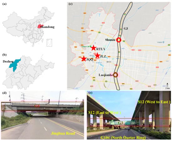
Figure 1.
Schematic diagram of the experimental sites: (a) position of Shandong Province in China; (b) position of Dezhou in Shandong Province; (c) map of Dezhou: inside the black frame is the G3 highway, the red circles are the locations of the two experimental sites, and the red five-pointed stars in the picture are the locations of three state control monitoring stations; (d) position and shape of G3 at Laojianhe; (e) position and shape of G3 at Shuniu.
2.2. Data Collection
The experiment used the DJI M600 UAV equipped with portable sensors to monitor the air quality. The placement of the instruments and fly routes of the UAV are shown in Figure 2a–c. The intake pipes were Teflon tubes, which can improve the sampling accuracy, and the inlets were placed in the windward direction, higher than the propellers, to avoid the potential influence. The wind tunnel experiment showed that inlets placed this way are the most effective [29].
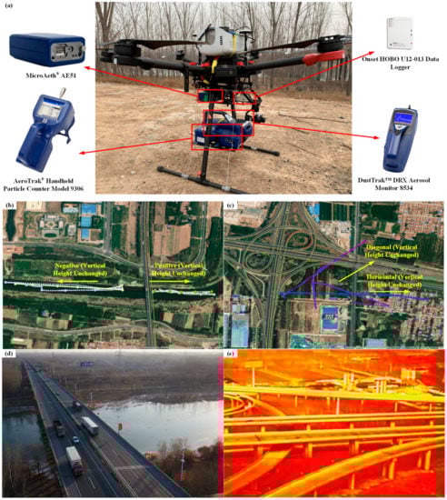
Figure 2.
Experimental equipment, flight path, and actual view of the experimental sites. (a) is the UAV platform and placement of each equipment; (b,c) are the flight paths in Laojianhe and Shuniu; (d) shows real shots from the UAV at Laojianhe; and (e) shows thermal image shots at Shuniu.
Flight modes include both vertical and horizontal. The vertical flight of 0–500 m was carried out at two locations. In order to avoid airflow interference and reduce the systematic error, the UAV hovered at different heights for 1–2 min and then took the average value to represent the concentration of the point. Horizontally, the flight route extended in the two directions perpendicular to the road, at the height of the highway elevation. The flying height at Laojianhe was 6 m, and the farthest distance away from the highway was 700 m (Figure 2b). In Shuniu, the flying height was 10 m, parallel to the height of the G3 elevation. Because there is another highway in this position, the flight route was first perpendicular to G3 and then diagonal, 45° across S12 (Figure 2c). At the same time, during the two experimental campaigns, the traffic volumes and composition were recorded using the DJI M200 UAV with high definition camera and infrared camera and then manually counted (Figure 2d–e).
The same pollutants were measured at two experimental sites, including PNs of the six size segments (0–0.3 μm, 0.3–0.5 μm, 0.5–1 μm, 1–3 μm, 3–5 μm, and 5–10 μm), PMs of the three size segments (1 μm, 2.5 μm, and 10 μm), and BC (880 nm). To achieve the above monitoring objectives, the DustTrak DRX Aerosol Monitor 8534 [30] was used to measure the PMs, the TSI AeroTrak Handheld Particle Counter 9306 was used to measure the PNs [31,32], and the Magee Scientific microAeth Model AE51 was used to measure the BC [30]. The technical parameters of each instrument are shown in Table 1.

Table 1.
Technical parameters and performance of the equipment.
Before the experiment, all the equipment was compared with the standard equipment from the state control monitoring station for 24 h to obtain the correction factor (Figure 3). The comparison between the portable equipment and the state control monitoring station showed a good correlation (R = 0.97 for PM and 0.88 for BC). The AeroTrak 9306 and DustTrak 8534 were zero-calibrated before use, and the AE51 was inspected for the attenuation (ATN, which scales from 0 to 100) of the transmitted light (wavelength: 880 nm) prior to use to determine if the filter membrane needed to be replaced. The equipment was turned on for 10 to 20 min before each flight for preheating, and the measurement was not started until the reading was stable. The measured meteorological parameters were temperature and relative humidity. The other hourly weather data used in this paper comes from the public library of the state control monitoring station (https://www.aqistudy.cn/), including wind speed and direction and weather conditions (Figure 1c).
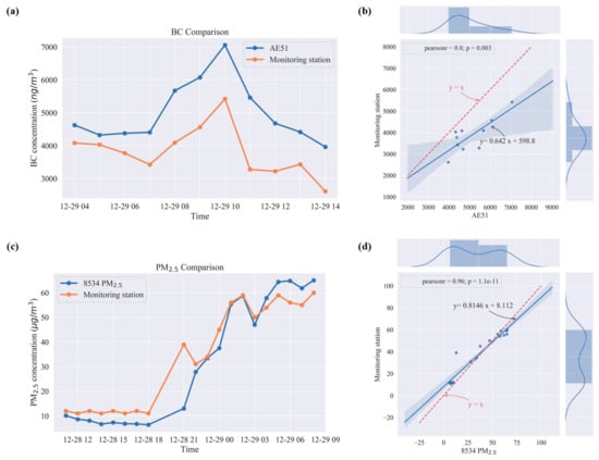
Figure 3.
Calibrations for PM2.5 and BC. (a,c) are the variations for BC and PM2.5 with the state control monitoring station; (b,d) are the regression curves used to calibrate.
The experiment was conducted in two campaigns, in winter and spring, to investigate variations in pollutants in different seasons. The first experiment was carried out from 28 December 2018 to 3 January 2019 with colder temperatures, clear skies most of the time and a shallower mixing layer. At that time, Dezhou still used central heating, which further increased the degree of pollution. The second experiment was carried out from 27 February 2019 to 1 March 2019. At that time, the temperature rose, the diffusion conditions gradually improved, and the central heating ended. Besides the meteorological conditions, the vegetation and pollutant characteristics were also different in both campaigns, giving a wide range of scenarios to be studied. Since the background concentration was not measured separately, there was also a lack of measurement of PN data in monitoring stations in China. Therefore, the minimum value of the concentration in each flight was extracted as the background value to eliminate its influence. After determining the background concentration of each flight separately, we subtracted the background concentration from the measured concentration at all measurement points of the flight to obtain the certain concentration after removing the background concentration. The outliers were removed using the 3σ rule.
3. Results and Discussion
During the whole experiment, 17 flights (12 at Laojianhe, 5 at Shuniu) were carried out, 88 sets of available concentration data records for PN, 48 for PM, and 99 for BC, were collected.
3.1. Meteorological and Traffic Flow Characteristics
Firstly, statistics of meteorological factors and traffic flow were calculated to distinguish the difference in different seasons. The average temperature in winter in Dezhou was 6.38 °C lower than that in spring and the peak temperature in winter was 1 h earlier than in spring. Humidity was basically the same in winter and spring. Meanwhile, the average wind level was 1.35 in winter and 1.63 in spring, which indicates that the diffusion conditions in spring were better than in winter. In winter there was mainly northeast wind and in spring southwest wind. In addition, there was no precipitation during the entire monitoring period. According to the counting results of the videos, the traffic volume in winter was 717–1317 veh/h and in spring 793–1107 veh/h. Since the vacation time of China New Year’s Day in 2019 was from 30 December 2018 to 1 January 2019, the traffic volume of highways during the holiday increased 3%–5% [33]. As a result, passenger car traffic increased sharply on 29 December. There was little change in winter and spring traffic. In addition, when analyzing the thermal image video, it was found that the tires of large trucks tend to have a significantly higher temperature than those of ordinary cars. Since tire wear is also one of the sources of particulate matters in the air [34], this phenomenon also indicates that large trucks will induce higher emissions. To verify whether the data was statistically different, a non-parametric hypothesis test was used to check for statistical differences. The results show that there was no significant difference (p > 0.05) in temperature and wind speed at the two locations. Only the relative humidity was different.
3.2. Spatial and Temporal Variations of Air Pollutants
The statistical description of the different locations was calculated (Table 2). Generally, the air pollutants at the transportation interchanges (Shuniu) were all significantly higher than at the suburban area (Laojianhe). The reason is that the traffic volume in Shuniu is larger, and the road structure is more complicated. Before and after entering the intersection, the traffic flow will go through uphill slopes, take sudden turns, and then go downhill. At the same time, the general speed limit of the ramp is 40 km/h, and that on the road is 120 km/h. The vehicles have to break before entering the ramp, and the wear of the brake and tire are one of the main sources of particles [35,36]. The results of the non-parametric hypothesis test showed that, except for PN0.3, other pollutants confirm the assumption that there are statistical differences between the two locations. Therefore, it can be considered that the main reasons for the differences in the pollutant concentrations at the two locations are factors other than meteorological parameters, such as traffic composition, volume, speed, density, and the surrounding built environment.
Table 2.
Statistical description for different locations.
3.2.1. Vertical Variation
The vertical profiles (Figure 4) have removed the background concentration. As can be seen from the figure, some vertical profiles have large fluctuations. At 120 m above the ground, the PN5, PN10, and PMs ascended suddenly at Shuniu, and the increment at 10 μm was the most obvious, while BC did not increase. The measurement periods of Shuniu’s two voyages correspond to a heavily polluted stage in Dezhou, and the PM10 of the state control monitoring station was as high as 225 μg/m3. Therefore, it is speculated that there was a polluted air mass passing over the area, composed mainly of coarse particles, which caused the large fluctuations in PN10 and PM10.
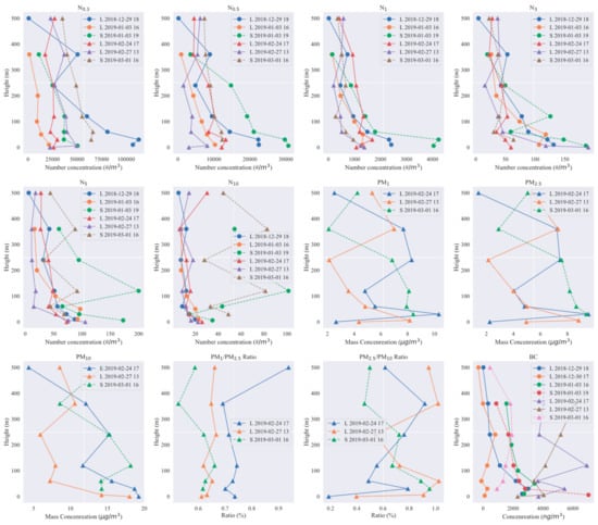
Figure 4.
Vertical profiles of each air pollutant. The black dotted line represents the position of the highway. The solid line refers to Laojianhe (L) and the dotted line to Shuniu (S). The dots in the lines are experiments in winter and the triangles are in spring.
Most air pollutants had a significant increase in altitude at the height of the highway. The statistical results show that, at 6 m–10 m above the ground, compared with the ground, PNs increased by 54.10%–247.95% and BC increased by 201.33%. This reflects the increase of pollutants on the highway at the same height, and this phenomenon was more obvious in winter due to the worse diffusion conditions. Furthermore, the finer particulate matter, the increment became more obvious, and the PN10 almost did not show any difference. In addition, the increase in the spring from 0 to 30 m was more obvious, and a significant increase could be observed in PN0.3,0.5, PM1,2.5, and BC.
There was a significant decrease in the concentrations of all the air pollutants, as the height above the ground increased. The decline rate decreased gradually with the increase of height and remained stable after 120 m. The standard deviation of the concentrations at 0–120 m was 0.6%–23.9% higher than that at 120–500 m, indicating that the concentration remained unchanged after 120 m. Different pollutants have different vertical profiles. The attenuations for PN0.3–PN3, PM1, PM2.5, and BC were more obvious. The coarse particles were more likely to be removed by dry deposition, and the variations were more stable, except for some abnormal values. The finer the particles, the more pronounced the attenuation with height. The attenuation of PN10 and PM10 was hard to notice. The reason is that the coarse particles are mainly formed by mechanical grinding and crushing activities, and can be removed faster by gravitational settling [17], while UFPs with less than 1 μm are emitted by the combustion sources, including traffic. PM variations were not as significant as PN changes with traffic because the vehicle-related particulate matter emissions were mainly UFPs with a slight weight, and hence not obvious in terms of mass concentration. Our results are consistent with other studies [37] showing that PMs and PNs do not always reflect road traffic emissions, that BC levels are proportional to traffic-related gaseous pollutants (such as CO, NO2, and NO), and that BC is directly related to traffic emissions and not affected by other particulate sources, as dust outbreaks and soil resuspension.
In order to further explore the gradient variations of air pollutants at different altitudes, a linear regression of concentration changes at every two altitudes was carried out, and the regression result R2 was plotted on the heatmap (Figure 5). When slope = 1, the variation rate of the two altitudes was basically the same; < 1 indicates that the rate of change at a higher altitude concentration was lower than that at a lower altitude, and vice versa.
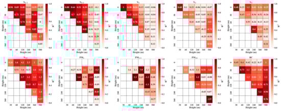
Figure 5.
The heatmaps of R2 for linear regression of concentration between two altitudes. The color in each figure represents the value of R2, and the number is the slope of the regression equation. The row number is the start altitude, and the column number is the end altitude.
As can be seen from Figure 5, the correlations for linear regression between 0–120 m were higher than others. Between 0–120 m, PN0.3-N1 had higher R2, indicating that the linear relationship between the two adjacent heights was stronger. Among them, 0–30 m had higher R2 in all PNs (except PN10), which means the concentration at 0 m had a good linear correlation with that at 30 m. The slope of the regression equation approached 1, suggesting that when the concentration at 0 m varied, the value at 30 m would have a similar variation. However, as the particle size increased, the change rate decreased gradually. The PN3–PN5 regression shows that the concentration increment of 30 m was smaller than the ground increment, indicating that the correlation between adjacent heights decreased with the increase of particle size. The variations between other altitudes were smaller than that of the ground. This also confirms the previous conclusion that the concentration of pollutants next to the highway has a significantly high value, but its maximum impact altitude was around 120 m in our experiment. PN0.3-PN1 had highly linear relationships in both adjacent altitudes (diagonal). As the end altitude increased, the correlation gradually decreased. The correlation of PN10 was higher in the regression when starting at 0 m, 60 m, and 120 m. Although it was not obvious in the analysis of the vertical profiles, almost all the profiles showed an increasing trend at the height of 60 m-120 m. The slope was 2.7, which means that when the concentration at 60 m changed, the variance at 120 m was 2.7 times higher. Similar patterns were found in PM1 and PM2.5, but the changing rate was lower. The change of BC was different from that of PNs and PMs. The correlation between 0 m and a higher altitude was higher, and the slope was around 1, which was consistent with the above mentioned conclusion that BC is more related to traffic emission.
3.2.2. Horizontal Variation
The variation of all pollutants in all horizontal voyages is displayed in Figure 6. Because background concentrations were removed, there was little difference in concentration level between the two locations. Generally, almost all pollutants were higher at the roadside and then decreased with the increment of distance. The attenuation distance was 200 m in Shuniu and 100 m in Laojianhe. However, the abnormally high concentration values were observed at both locations. At Laojianhe, all pollutants expect PN0.3 had a high concentration 200 m east of the highway, which was due to a biological forage company that produces particles and dust during the biofeed fermentation process. 300 m to the west, there is an automobile repair and accessory industrial park which contributed to the abnormally high concentration. At Shuniu, there were high concentrations of almost all PNs 200 m to the east, indicating the emissions were from enterprises and urban roads. Furthermore, 400 m to the east, PNs were even higher, which was due to the biomass combustion activities (resident heating, cooking, etc.) from a nearby village. After excluding other additional sources, it can be concluded that the PNs usually spread to 100 m and then began to decline, which is similar to what was reported in previous studies [12,15,20]. Among them, due to the formation of new particles in traffic-related particles, PN0.3 gradually increased within 0–100 m and could last up to 200 m. The attenuation of PN1-PN5 was more prominent. Differently, BC began to decay rapidly after 50 m. On January 3 at Laojiange, the concentration was highest but attenuated rapidly by 85% at around 50 m east of the highway and remained basically unchanged afterward, unlike that of PNs, which did not decay to the background level until 200 m.
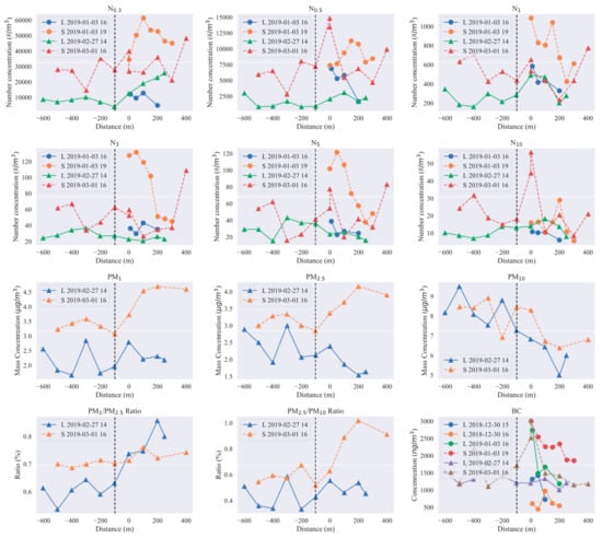
Figure 6.
Horizontal profiles of the air pollutants.
The wind direction has a significant influence on the diffusion of pollutants. In spring, both sides of the highway were monitored so that the influence of the wind could be explored. At Laojianhe, the wind speed was 2 m/s and came from the southwest. Thus, the western side of highway was affected by an upwind direction (the negative direction in Figure 6). The PNs in the upwind direction remained basically unchanged and decreased slightly 200 m away from the highway. However, in the downwind direction, PN0.3-PN1 were 66%-381% higher than the upwind at 100 m, but there was no significant difference between the coarser particles. The PM1/PM2.5 ratio in the upwind direction was much lower than in the downwind direction, implying that PM1 represented a significant portion of PM2.5 near traffic sources [38,39].
After crossing another highway, the concentration of each air pollutant increased significantly. At Shuniu, during the experiment, the wind came from the southwest. According to the aforementioned experimental scheme, the horizontal direction was eastward, perpendicular to G3, and the diagonal direction was to the northeast. In the diagonal direction, 0–300 m was between G3 and S12, and after 400 m, it crossed S12 and continued to fly forward in the same direction as the wind. Therefore, the PNs in all sizes, from 0 to 300 m, were gradually attenuated, with a decrease of 35–81%. However, at 400 m, the PNs increased by 69–289% when compared with the values measured at 300 m, with PN10 increasing the least. Similarly, the PMs increased by 7–28%, and BC increased by 101%.
The formation of new particles was observed at both locations, almost always within 100 m of the roadside. PN0.3 at Shuniu in winter and at Laojianhe in spring increased with distance, indicating that traffic will affect the formation of new particles in the ultrafine particle size through nucleation. At Laojianhe, PN0.3 was lowest at the roadside and then gradually increased with the variations in Shuniu in winter. Because the formation of new particles was mainly less than 20 nm [40], the concentration increased with distance only in PN0.3. In these two voyages with new particle formations, although the temperature varied significantly with the seasons, the relative humidity was not much different and was lower than in all other voyages. Previous studies [41] have also shown that in the case of low humidity, strong solar radiation, and low rainfall, new particle formation is more likely to occur, further verifying the conclusion.
Different pollutants showed different decay variations, and BC was the most affected by traffic, followed by PNs and PMs, which is consistent with the above analysis. In winter, at Laojianhe, the BC concentration at 4:00 p.m. on 30 December 2018 was significantly higher than that at 3:00 p.m., but decreased by 49% to the same level at 3:00 p.m. 100 m east of the highway. This further shows that BC can clearly reflect the variations of the traffic-related pollutants.
4. Conclusions
To fill in the void of three-dimensional in situ monitoring of air pollution near roads, this paper investigated the variation of air pollutants near elevated highways with different road configurations. Based on the UAV air monitoring platform, the vertical and horizontal profiles near the elevated highway were measured. The field experiments showed that almost all the pollutants dropped to the background level after 100 m horizontally, which is consistent with former studies [15,16], but at Shuniu, with a more complicated road configuration, the distance extended to 200 m, and the general pollution level was also higher than at Laojianhe, a suburban area with a single elevated highway. Different road configurations have important effects on the diffusion of traffic-related air pollutants, and road configurations must be taken into consideration to estimate traffic-related pollution exposure more accurately. Here are some major findings:
- The vertical profiles showed that PNs and BC had significant increases at the height of the elevated highway, i.e., 6 m–10 m above the ground, which has been neglected in the previous ground-based studies. Compared with the ground, at the elevated highway altitude, PNs increased by 54%–248% and BC increased by 201%.
- There is a significant decrease in the concentrations of all the air pollutants as the height above the elevated highway increases. The decline rate decreases gradually with the increase of height and remains stable after 120 m.
- The R2 heatmap for the linear regressions between every altitude showed that the linear relationship between 0–120 m was higher than the others. As the altitude increases, the relationship gradually weakens, and between 0–30 m the R2 is higher in all PNs (except PN10).
- In the horizontal profiles, almost all pollutants were higher at the roadside and then decreased with the increment of distance. PNs spread to 100 m and then began to decline, BC began to decay rapidly after 50 m, but PMs showed less variation.
- The wind direction has a significant influence on the diffusion of pollutants. After crossing another highway, PNs increased by 69–289%, PMs by 7–28%, and BC by 101%, indicating that the traffic emissions have a huge impact on the air quality above the highway, especially on UFPs.
- The formation of new particles was observed at both locations, as PN3 increased with distance horizontally, and almost always within 100 m of the roadside.
- Different pollutants showed different decay variations horizontally and vertically, and BC was most affected by traffic, followed by PNs and PMs. This is consistent with the previous studies.
However, the dataset in this study is relatively small. To improve the accuracy of the exposure estimates of near-road pollutants, further monitoring of changes in pollutant gradients along the highway should be added to sample multiple times in different contexts (e.g., several periods during the year). Furthermore, three-dimensional distribution patterns of air pollutants should be studied to help validate and enhance roadside emission dispersion models.
Author Contributions
The authors confirm the contributions to the paper as follows: conceptualization, R.C., B.L., and Z.-R.P.; data curation, R.C. and B.L.; formal analysis, R.C. and B.L.; funding acquisition, Z.-R.P.; methodology, R.C., B.L., and S.T.; supervision, Z.-R.P.; writing and original draft, R.C., B.L., and H.-W.W.; writing, review, and editing, S.T., Z.-R.P., and H.-D.H. All authors have read and agreed to the published version of the manuscript.
Funding
This research was funded in part by the National Planning Office of Philosophy and Social Science (16ZDA048); the National Key R&D Program of China, grant number 2016YFC0200500; the Science and Technology Project of Guangzhou, grant number 201803030032; and the National Natural Science Foundation of China, grant number 11672176.
Conflicts of Interest
The authors declare no conflict of interest.
References
- Devaraj, S.; Tiwari, S.; Ramaraju, H.K.; Dumka, U.C.; Sateesh, M.; Parmita, P.; Shivashankara, G.P. Spatial and Temporal Variation of Atmospheric Particulate Matter in Bangalore: A Technology-Intensive Region in India. Arch. Environ. Contam. Toxicol. 2019, 77, 214–222. [Google Scholar] [CrossRef] [PubMed]
- Zhou, M.; Wang, H.; Zeng, X.; Yin, P.; Zhu, J.; Chen, W.; Li, X.; Wang, L.; Wang, L.; Liu, Y.; et al. Mortality, morbidity, and risk factors in China and its provinces, 1990–2017: A systematic analysis for the Global Burden of Disease Study 2017. Lancet 2019, 394, 1145–1158. [Google Scholar] [CrossRef]
- Guo, Y.; Jia, Y.; Pan, X.; Liu, L.; Wichmann, H.-E. The association between fine particulate air pollution and hospital emergency room visits for cardiovascular diseases in Beijing, China. Sci. Total Environ. 2009, 407, 4826–4830. [Google Scholar] [CrossRef]
- The Lancet Respiratory Medicine Efforts to tackle air pollution should focus on accountability. Lancet Respir. Med. 2019, 7, 553. [CrossRef]
- Barnes, J.H.; Chatterton, T.J.; Longhurst, J.W.S. Emissions vs exposure: Increasing injustice from road traffic-related air pollution in the United Kingdom. Transp. Res. Part D Transp. Environ. 2019, 73, 56–66. [Google Scholar] [CrossRef]
- Barone, R.E.; Giuffrè, T.; Siniscalchi, S.M.; Morgano, M.A.; Tesoriere, G. Architecture for parking management in smart cities. IET Intell. Transp. Syst. 2014, 8, 445–452. [Google Scholar] [CrossRef]
- Dockery, D.W.; Stone, P.H. Cardiovascular Risks from Fine Particulate Air Pollution. N. Engl. J. Med. 2007, 356, 511–513. [Google Scholar] [CrossRef]
- Pope, C.A., III. Lung Cancer, Cardiopulmonary Mortality, and Long-term Exposure to Fine Particulate Air Pollution. JAMA 2002, 287, 1132. [Google Scholar] [CrossRef]
- Gan, W.Q.; Koehoorn, M.; Davies, H.W.; Demers, P.A.; Tamburic, L.; Brauer, M. Long-Term Exposure to Traffic-Related Air Pollution and the Risk of Coronary Heart Disease Hospitalization and Mortality. Environ. Health Perspect. 2011, 119, 501–507. [Google Scholar] [CrossRef]
- Zheng, X.; Zhang, S.; Wu, Y.; Zhang, K.M.; Wu, X.; Li, Z.; Hao, J. Characteristics of black carbon emissions from in-use light-duty passenger vehicles. Environ. Pollut. 2017, 231, 348–356. [Google Scholar] [CrossRef]
- Zhu, Y.; Kuhn, T.; Mayo, P.; Hinds, W.C. Comparison of daytime and nighttime concentration profiles and size distributions of ultrafine particles near a major highway. Environ. Sci. Technol. 2006, 40, 2531–2536. [Google Scholar] [CrossRef] [PubMed]
- Durant, J.L.; Ash, C.A.; Wood, E.C.; Herndon, S.C.; Jayne, J.T.; Knighton, W.B.; Canagaratna, M.R.; Trull, J.B.; Brugge, D.; Zamore, W.; et al. Short-term variation in near-highway air pollutant gradients on a winter morning. Atmos. Chem. Phys. 2010, 10, 5599–5626. [Google Scholar] [CrossRef]
- Hu, S.; Fruin, S.; Kozawa, K.; Mara, S.; Paulson, S.E.; Winer, A.M. A wide area of air pollutant impact downwind of a freeway during pre-sunrise hours. Atmos. Environ. 2009, 43, 2541–2549. [Google Scholar] [CrossRef] [PubMed]
- Rakowska, A.; Wong, K.C.; Townsend, T.; Chan, K.L.; Westerdahl, D.; Ng, S.; Močnik, G.; Drinovec, L.; Ning, Z. Impact of traffic volume and composition on the air quality and pedestrian exposure in urban street canyon. Atmos. Environ. 2014, 98, 260–270. [Google Scholar] [CrossRef]
- Padró-Martínez, L.T.; Patton, A.P.; Trull, J.B.; Zamore, W.; Brugge, D.; Durant, J.L. Mobile monitoring of particle number concentration and other traffic-related air pollutants in a near-highway neighborhood over the course of a year. Atmos. Environ. 2012, 61, 253–264. [Google Scholar] [CrossRef] [PubMed]
- Patton, A.P.; Perkins, J.; Zamore, W.; Levy, J.I.; Brugge, D.; Durant, J.L. Spatial and temporal differences in traffic-related air pollution in three urban neighborhoods near an interstate highway. Atmos. Environ. 2014, 99, 309–321. [Google Scholar] [CrossRef]
- Ginzburg, H.; Liu, X.; Baker, M.; Shreeve, R.; Jayanty, R.K.M.; Campbell, D.; Zielinska, B. Monitoring study of the near-road PM 2.5 concentrations in Maryland. J. Air Waste Manag. Assoc. 2015, 65, 1062–1071. [Google Scholar] [CrossRef]
- Pérez, N.; Pey, J.; Cusack, M.; Reche, C.; Querol, X.; Alastuey, A.; Viana, M. Variability of Particle Number, Black Carbon, and PM10, PM2.5, and PM1 Levels and Speciation: Influence of Road Traffic Emissions on Urban Air Quality. Aerosol Sci. Technol. 2010, 44, 487–499. [Google Scholar] [CrossRef]
- You, S.; Yao, Z.; Dai, Y.; Wang, C.-H. A comparison of PM exposure related to emission hotspots in a hot and humid urban environment: Concentrations, compositions, respiratory deposition, and potential health risks. Sci. Total Environ. 2017, 599–600, 464–473. [Google Scholar] [CrossRef]
- Zhu, Y.; Hinds, W.C.; Kim, S.; Sioutas, C. Concentration and Size Distribution of Ultrafine Particles Near a Major Highway. J. Air Waste Manag. Assoc. 2002, 52, 1032–1042. [Google Scholar] [CrossRef]
- Shen, J.; Gao, Z. Commuter exposure to particulate matters in four common transportation modes in Nanjing. Build. Environ. 2019, 156, 156–170. [Google Scholar] [CrossRef]
- Elen, B.; Peters, J.; Poppel, M.; Bleux, N.; Theunis, J.; Reggente, M.; Standaert, A. The Aeroflex: A Bicycle for Mobile Air Quality Measurements. Sensors 2012, 13, 221–240. [Google Scholar] [CrossRef] [PubMed]
- Villa, T.F.; Salimi, F.; Morton, K.; Morawska, L.; Gonzalez, F. Development and validation of a UAV based system for air pollution measurements. Sens. Switz. 2016, 16, 2016. [Google Scholar] [CrossRef] [PubMed]
- Alvear, O.; Zema, N.R.; Natalizio, E.; Calafate, C.T. Using UAV-Based Systems to Monitor Air Pollution in Areas with Poor Accessibility. J. Adv. Transp. 2017, 2017, 1–14. [Google Scholar] [CrossRef]
- Haas, P.Y.; Balistreri, C.; Pontelandolfo, P.; Triscone, G.; Pekoz, H.; Pignatiello, A. Development of an Unmanned Aerial Vehicle UAV for Air Quality Measurement in Urban Areas. Available online: https://arc.aiaa.org/doi/abs/10.2514/6.2014-2272 (accessed on 7 February 2020).
- Yang, Y.; Zheng, Z.; Bian, K.; Song, L.; Han, Z. Real-Time Profiling of Fine-Grained Air Quality Index Distribution Using UAV Sensing. IEEE Internet Things J. 2018, 5, 186–198. [Google Scholar] [CrossRef]
- Villa, T.F.; Gonzalez, F.; Miljievic, B.; Ristovski, Z.D.; Morawska, L. An Overview of Small Unmanned Aerial Vehicles for Air Quality Measurements: Present Applications and Future Prospectives. Sensors 2016, 16, 1072. [Google Scholar] [CrossRef]
- Baldauf, R.; Thoma, E.; Hays, M.; Shores, R.; Kinsey, J.; Gullett, B.; Kimbrough, S.; Isakov, V.; Long, T.; Snow, R.; et al. Traffic and Meteorological Impacts on Near-Road Air Quality: Summary of Methods and Trends from the Raleigh Near-Road Study. J. Air Waste Manag. Assoc. 2008, 58, 865–878. [Google Scholar] [CrossRef]
- Li, B.; Cao, R.; Wang, Z.; Song, R.-F.; Peng, Z.-R.; Xiu, G.; Fu, Q. Use of Multi-Rotor Unmanned Aerial Vehicles for Fine-Grained Roadside Air Pollution Monitoring. Transp. Res. Rec. J. Transp. Res. Board 2019, 2673, 169–180. [Google Scholar] [CrossRef]
- Gómez-Moreno, F.J.; Artíñano, B.; Ramiro, E.D.; Barreiro, M.; Núñez, L.; Coz, E.; Dimitroulopoulou, C.; Vardoulakis, S.; Yagüe, C.; Maqueda, G.; et al. Urban vegetation and particle air pollution: Experimental campaigns in a traffic hotspot. Environ. Pollut. 2019, 247, 195–205. [Google Scholar] [CrossRef]
- Hussein, T.; Boor, B.E.; dos Santos, V.N.; Kangasluoma, J.; Petäjä, T.; Lihavainen, H. Mobile Aerosol Measurement in the Eastern Mediterranean—A Utilization of Portable Instruments. Aerosol Air Qual. Res. 2017, 17, 1875–1886. [Google Scholar] [CrossRef]
- McGarry, P.; Morawska, L.; He, C.; Jayaratne, R.; Falk, M.; Tran, Q.; Wang, H. Exposure to Particles from Laser Printers Operating within Office Workplaces. Environ. Sci. Technol. 2011, 45, 6444–6452. [Google Scholar] [CrossRef] [PubMed]
- Gen, L. Attention, New Year’s Day Travel Must See, Dezhou High-Speed Traffic Police Released Two Announcements and a Reminder. 2018. Available online: http://www.dezhoudaily.com/p/1434074.html (accessed on 7 February 2020).
- Panko, J.; Hitchcock, K.; Fuller, G.; Green, D. Evaluation of Tire Wear Contribution to PM2.5 in Urban Environments. Atmos. Basel 2019, 10, 99. [Google Scholar] [CrossRef]
- Abu-Allaban, M.; Gillies, J.A.; Gertler, A.W.; Clayton, R.; Proffitt, D. Tailpipe, resuspended road dust, and brake-wear emission factors from on-road vehicles. Atmos. Environ. 2003, 37, 5283–5293. [Google Scholar] [CrossRef]
- Panko, J.M.; Chu, J.; Kreider, M.L.; Unice, K.M. Measurement of airborne concentrations of tire and road wear particles in urban and rural areas of France, Japan, and the United States. Atmos. Environ. 2013, 72, 192–199. [Google Scholar] [CrossRef]
- Reche, C.; Querol, X.; Alastuey, A.; Viana, M.; Pey, J.; Moreno, T.; Rodríguez, S.; González, Y.; Fernández-Camacho, R.; de la Rosa, J.; et al. New considerations for PM, Black Carbon and particle number concentration for air quality monitoring across different European cities. Atmos. Chem. Phys. 2011, 11, 6207–6227. [Google Scholar] [CrossRef]
- Munir, S. Analysing Temporal Trends in the Ratios of PM2.5/PM10 in the UK. Aerosol Air Qual. Res. 2017, 17, 34–48. [Google Scholar] [CrossRef]
- Xu, G.; Jiao, L.; Zhang, B.; Zhao, S.; Yuan, M.; Gu, Y.; Liu, J.; Tang, X. Spatial and Temporal Variability of the PM2.5/PM10 Ratio in Wuhan, Central China. Aerosol Air Qual. Res. 2017, 17, 741–751. [Google Scholar] [CrossRef]
- O’Dowd, C.D.; Aalto, P.; Hämeri, K.; Kulmala, M.; Hoffmann, T. Atmospheric particles from organic vapours. Nature 2002, 416, 497–498. [Google Scholar] [CrossRef]
- Qi, X.; Ding, A.; Nie, W.; Chi, X.; Huang, X.; Xu, Z.; Wang, T.; Wang, Z.; Wang, J.; Sun, P.; et al. Direct measurement of new particle formation based on tethered airship around the top of the planetary boundary layer in eastern China. Atmos. Environ. 2019, 209, 92–101. [Google Scholar] [CrossRef]


© 2020 by the authors. Licensee MDPI, Basel, Switzerland. This article is an open access article distributed under the terms and conditions of the Creative Commons Attribution (CC BY) license (http://creativecommons.org/licenses/by/4.0/).