Abstract
Trees provide a broad amount of ecosystem services in urban areas. Although it is well documented that trees are essential for the well-being and livability of cities, trees are often not evenly distributed. Studies have found that urban residents with a deprived socioeconomic status are associated with a lower coverage and access to urban trees in their communities, yet a fair distribution of trees contributes to the sustainability and resilience of cities. In this context, the environmental justice movement seeks to ensure equal distribution of green infrastructure and its benefits throughout a territory. The objective of this study is threefold: (i) to determine whether urban trees in Guadalajara, Mexico, are distributed equally; (ii) to assess the association between urban trees and socioeconomic status; and (iii) to introduce compositional data analysis to the existing literature. Due to the compositional nature of the data, compositional analysis techniques are applied. We believe this novel approach will help define the proper management of data used in the literature. The outcomes provide insights for urban planners working towards the Sustainable Development Goals to help eradicate the uneven distribution of urban trees in cities.
1. Introduction
The global phenomena of rapid urbanization has important consequences in the livability and environment of cities’ inhabitants [1,2] and whose degree of impact depends on their development level [3]. Solid waste generation [4,5], water scarcity and pollution [6,7], air pollution [8,9], floods [10,11] and the heat island effect [12,13] are some of the consequences of this phenomenon. To mitigate these and make cities more resilient and sustainable, different authorities around the world have implemented green infrastructure into their political agendas. Commonly, these agendas are aligned with the Sustainable Development Goals (SDGs) issued by the United Nations as goals for 2030 [14,15,16]. If well planned, green spaces (such as parks, community gardens, green roofs, greenways, sporting fields and street trees, among others) have the potential to promote sustainable and resilient cities [14,17] through their ecosystem services [18,19].
Urban trees provide cities and their inhabitants with different ecosystem services, including improvement of air quality [20], mitigation of heat island effects [21,22], filtration and reduction of storm water runoffs [23], moderation of urban temperatures [24,25], reduction of noise pollution [26] and a habitat for different species [27], among others. These services have socio-economic implications, such as an increase in property values [28], reduction of crime [29], visual aesthetics in high-speed corridors and in business districts [30,31], increased social cohesion [32], increased longevity of elders [33] and mitigation of health problems [34], among others.
Despite the wide recognition of ecosystem services generated by urban green infrastructure to the livability of cities, studies have revealed that these are unevenly distributed [18,19,35]. This unequal distribution is unique for each urban context and might be caused by different reasons, including the history of land development, changes in land-use, the design philosophy, class history, ethno-racial inequalities, state oppression, state-led policies to increase property values, lack of economic resources of cities and households to maintain and develop green infrastructures, community resistance, top–down policies and the absence of public policies based on justice [18,35,36,37,38,39,40,41,42].
The environmental justice movement born in 1980 in the United States [36,43] has generated a large amount of literature highlighting the absence of a social component (considered one of the three pillars of sustainable development, together with the economic and environmental pillars) in the planning and allocation of infrastructure and socioeconomic activities. In this sense, several studies have shown that communities of low socioeconomic status have a greater exposure to environmental hazards and health-related problems.
Environmental justice research is currently focusing on the study of the distribution of green amenities, to analyze who actually receives the environmental benefits [36]. Most research has focused only on the equitable distribution of, and access to, urban parks and recreational facilities [44,45]. Racial and ethnic minorities often have lower access to parks and green spaces, as shown by studies in Canada [46], Ecuador [47], Spain [35], United States [18,48], Colombia [49], Portugal and Estonia [17], among others. Thus, there is a strong relationship between inhabitants of high socioeconomic status and accessibility to green spaces.
Various studies have analyzed the spatial distribution of urban trees from an environmental justice perspective, using different approaches. Using remote sensing techniques and spatial error regression models, Landry and Chakraborty [44] found an unequal distribution of street trees with regard to ethnicity, income and housing tenure in Tampa, Florida, USA. The authors found that high-income neighborhoods have more land available to plant trees and are more willing to do so. In turn, the value of property and the area increase, making it more attractive for public and private investments. Using a walking distance approach, Zhou and Kim [50] confirm the inequity hypothesis; namely, that minorities have less tree canopy access in six cities of Illinois. In Washington D.C., Chuang and colleagues [51] used a multi-stage regression analysis to identify the association between tree canopy and socioeconomic status over a period of twenty years. The authors found that high socioeconomic status is not necessarily a predictor of a high canopy of trees. Krafft and Fryd [52] performed a spatiotemporal analysis of patterns of tree canopy and their relationship to income, house tenure and level of education, in Melbourne, Australia. The authors found income to be the variable that most influences tree cover inequality. Hernández and Villaseñor [53] incorporated the diversity of trees in their study (i.e., native and exotic), and their relationship with the socioeconomic level of people in Santiago de Chile. Applying non-parametric permutational multivariate analysis of variance, the authors found that areas with high socioeconomic status have a greater diversity of tree species and a larger amount of trees. The authors mention that about 45%–70% of trees are privately owned. The socioeconomic level of each household influences the behavior towards tree planting and removal in Santiago. Wang and Qiu [54] took into account the location in which the trees are planted (i.e., boulevards and parks) and its relationship with socioeconomic status and with different modes of transportation in Edmonton, Canada. Applying spatial regression models and the container approach, Wang and Qiu found that neighborhoods with a high median income have higher number of trees in parks. Likewise, people who choose to walk tend to have greater availability of trees. According to Wang and Qiu, an environmental improvement could be achieved through policies promoting an active and healthy lifestyle. Finally, Baró and colleagues [42] considered ecosystem services provided by urban trees in their study of Barcelona. Using i-Tree Eco and through bivariate, multivariate and regression analyses, the authors found no association between the services provided by street trees and income. According to the authors, the different historical processes of the city of Barcelona in its urban development might have influence on tree location.
To a large extent, studies have focused on the spatial distribution of green infrastructure and their relationship with different socio-economic groups through multivariate statistical analysis (e.g., principal component analysis, cluster analysis and regression techniques), omitting the compositional nature of their data e.g., [42,44,49,54,55,56]; however, this omission might have caused spurious and bias results. With compositional data (CoDa), the importance of the analysis is not in the absolute values as such; rather, the interest of the data is in its relative information, which is located between the components. Thus, using standard statistical methods to analyze compositional data may lead to biased results. To avoid this, data should be transformed into Aitchison’s geometry [57,58,59].
The present study is based on the first (and only) census of trees conducted in 2018 in the city of Guadalajara, and considers the compositional nature of the data, with three main aims: (i) to determine whether or not urban trees in Guadalajara are distributed equally among its neighborhoods and urban districts; (ii) to assess whether or not there is an existing relationship between the availability of trees exclusive for inhabitants with high socioeconomic status; and (iii) to introduce compositional data analysis into the existent literature. The outcomes of this study provide insights for urban planners to eradicate the existent disparities of urban trees in the city.
2. Materials and Methods
2.1. Case Study Description: Guadalajara, Jalisco, Mexico
Guadalajara is located in western Mexico and is the capital of the state of Jalisco. It was founded in 1542 by the Spaniards in the proximities of the San Juan de Dios River (which corresponds to the current Independencia Causeway) under a clear social division: the Spaniards on the west side of the river, and the indigenous people on the east side of the river. The city has approximately 1.4 million inhabitants in an area of 13,421 hectares and an average density of 104.5 inhabitants per hectare. Households in the city have an average of four inhabitants. Most of the land in the city is already urbanized and is mostly private property [60].
To promote sustainable development, the municipality of Guadalajara decided to incorporate and link the objectives of the SDGs with the municipal development plans, and in particular, in the 2016–2018 and 2018–2021 municipal development plans. Guadalajara is also part of different national and international networks who seek to implement actions against climate change, such as; the C40 Cities Climate Leadership Group; the global mayors’ pact for climate and energy; and the Alliance for Climate Action of the Metropolitan Area of Guadalajara (ACA-GDL), among others [61,62].
The municipal development plans are based on an actual diagnosis of the city and aim to establish base points towards the fulfillment of the SDGs. The initial diagnosis found 929,349 urban trees, of which 44% are in public roads (sidewalks, ridges and roundabouts), 35% in urban blocks and 21% in urban forests, parks and gardens. In order to reach the SDGs by 2030, the municipality has set two indicators. The first indicator is the rate of native trees planted with respect to the previous year, and it has 0% as base point and 90% as its goal. The second indicator is the percentage of maintenance and trees in public spaces, and it has 3% as a base point and 90% as its goal. According to the municipal government, the latter will be achieved mainly through two actions plans: tree planting by government investment, and tree adoption programs in conjunction with the private initiative.
2.2. Datasets
The tree dataset was obtained from the first and only census realized by the city government on June 2018. The information is open access and it is available in shapefile format [63]. This format stores the geometric location information (i.e., latitude and longitude) of each tree in the city and is projected as points (coordinate system WGS84/UTM Zone 13N). The dataset contains different attributes, such as trees by location type (i.e., urban blocks, streets, parks and gardens), canopy diameter and trees height. ArcMap 10.2.2 [64] was used to view and process the tree data set. Depending on the spatial location, this software enables the management datasets at different urban scales (e.g., neighborhood and district). Moreover, with ArcMap classification methods (i.e., Jenks Natural Breaks) and to better illustrate the methodology used in this study, four intervals were formed with respect to the height and diameter of the trees canopy [65].
The territorial boundaries of Guadalajara (395 neighborhoods and 7 urban districts) were obtained from the online mapping service of the city government [66] and are shown in Figure 1.
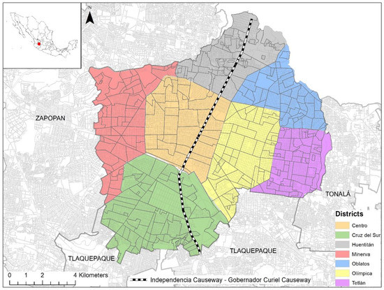
Figure 1.
Territorial boundaries of Guadalajara, Jalisco, Mexico. Dotted line corresponds to Independencia Causeway and Gobernador Curiel Causeway.
The socio-economic variables were obtained from the national population census elaborated by the National Institute of Statistics and Geography (INEGI) at urban block level. The cartographic base was elaborated from the urban blueprint maps, in digital format previously georeferenced by the INEGI [67]. In these maps, urban blocks are labeled with an identification code. With the latter, it is possible to link and process the population census variables in ArcMap. As the INEGI does not have an indicator to measure income, we considered households owning different goods as an approximation (Table 1), using information of the last census, taken in 2010 [68]. The variables considered in this study reflect the purchasing power of households, particularly households owning a car. In Latin American countries, car ownership represents a symbol of status [69]. In addition, the principles of confidentiality established by INEGI at an urban block level are not violated with these variables [70].

Table 1.
Socio-economic variables. Considered as an approximation of income.
Descriptive statistical analyses were performed using R [71], Rstudio [72] and CoDaPack [73]. The latter is a specialized software for compositional data treatment.
2.3. A Compositional Data Analysis Approach
The compositional analysis approach focuses on studying data that are part of a whole (e.g., are positive), and the importance of the information lies in the relative information between its components rather than in the absolute values [74,75]. Compositional data are commonly (but not necessary) expressed in a closed form, such as percentages or proportions adding up to 1% or 100%, depending on the case [58].
Analysis of compositional data in a raw form using standard statistical tools may lead to spurious correlations and consequently, to wrong conclusions [57,58,59]. Further consequences can be found in Pearson [76], Chayes [77], Aitchison [78,79], Rock [80] and Rollinson [81].
The sample space of compositional data is called the simplex [75]. The D-part simplex is defined as in Equation (1):
For explanatory purposes, Equation (1) shows one compositional vector of positive D-parts (carrying only relative information) that sum up to k. Zero components are not allowed and require special treatment [82]. Ignoring the compositional character of the data might lead to spurious correlations.
To overcome the consequences of working with compositional data, Aitchison [79] proposed an algebraic-geometrical structure for the Simplex (now called Aitchison geometry). Based on this structure, the compositions can be expressed as coordinates formed by log-ratios of compositional parts (log-ratio approach). The use of coordinates preserve the principles of compositional data, such as scale invariance, permutation invariance and sub-compositional coherence [74]. Once the compositions have been expressed into coordinates, standard statistical tools based on the Euclidean distance can be used without a problem.
In this sense, Aitchison introduced the additive log-ratio (alr) and centered log-ratio (clr) coordinates, and Egozcue et al. [83] introduced the isometric log-ratio (ilr) (which is also known as orthonormal log-ratio, olr). Each of these coordinates has unique characteristics, and their use depends on the desired analysis [58].
In this study, the tree dataset is a sample of compositional vectors; each compositional vector is a neighborhood, and the different parts of each composition correspond to the different attributes of trees (Table 2).

Table 2.
Compositional parts by trees attributes.
2.4. Simplex Visualization
The Simplex (sample space of compositional data) leads to different visual structures depending on the number of parts in the compositions. For D = 2, it can be displayed as a line segment; for D = 3, as a triangle (ternary diagram); and for D = 4, as a tetrahedron. It is not possible to display more than four parts. However, the mathematical structure and the operations defined in it are valid for D ≥ 4 [57]. In this study, the compositions are displayed in a tetrahedron.
2.5. Principal Component Analysis
Multivariate analysis of high dimensional data can lead to collinearity problems. Principal Component Analysis (PCA) creates a new set of independent and uncorrelated variables that capture the maximum explained variability of the original data [84]. Due to the compositional nature of the data, it was necessary to perform PCA using clr coordinates (Equation (2)).
PCA results are traditionally displayed in a biplot. Gabriel [85] introduced this tool, and Aitchison [86] adapted it for compositional data. The clr coordinates are recommended for performing a compositional biplot (also called as clr-biplot) [87]:
where:
The geometric mean g(X) in Equation (2) is considered by row (i.e., by sample).
2.6. Cluster Analysis
Cluster analysis groups observations that are similar to each other regarding some criteria. Different observations belonging to the same cluster will be very similar and will be different from observations belonging to other clusters. In this study, a hierarchical clustering method was applied; this method is a bottom–up agglomerative clustering. Each observation forms one class, and subsequently, each observation clusters with others until one cluster containing all observations is formed [58]. This study considers Ward’s hierarchical clustering, which is based on the sum of squares criterion [88].
To apply this descriptive method, the ilr/olr coordinates based on balances are used. Balances are a particular form of ilr/olr coordinates. The procedure to obtain these balances is called Sequential Binary Partition (SBP), which is a practical tool to set an orthonormal basis that is interpretable for the user. Balances are built in a hierarchical manner. As the first step, the compositional parts are divided in two groups, after which the new groups are divided into another set of new groups. This process is followed until the groups contain only one part. The resulting number of divisions will be D − 1. In Table 3, the parts of each group in each partition is defined by +1 and −1. Zero indicates that the part is not considered in the partition. The expression of the coordinates of a composition with respect to an orthogonal basis is represented as x*. For further information, please see Egozcue and Pawlowsky [89]. As a result of this approach, and in order to depict this method, the SBP of trees by attribute is shown in Table 3, and the ilr/olr coordinates in Equations (3a)–(3c) by location type, height and diameter, respectively.

Table 3.
Sequential Binary Partition (SBP) of trees by attribute.
2.7. Linear Regression
Regression analysis was then applied to find the association between trees and socioeconomic variables. The ilr/olr coordinates are real variables and allow standard linear regression techniques to be used, as shown in Equation (4). This study considers urban tree coordinates as response variables, and socioeconomic variables as explanatory variables (covariates). To be congruent with the method, the compositional character of each socioeconomic covariate described in Section 2.2 is considered as well (Table 4). A p-value of ≤0.05 was used to indicate significance:

Table 4.
Covariate variables in the regression analysis.
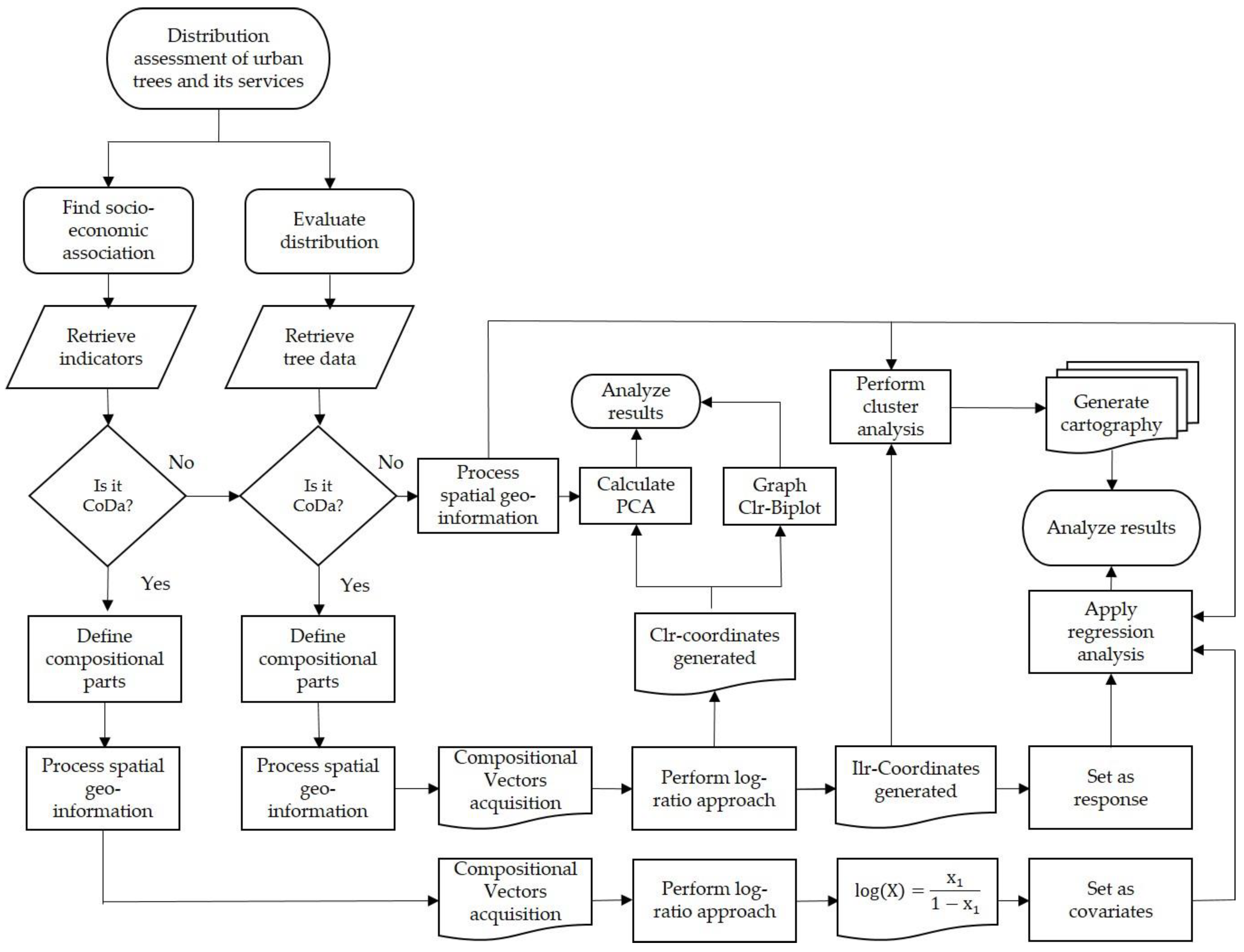
Finally, Figure 2 shows the flow chart detailing the process followed to perform this study.
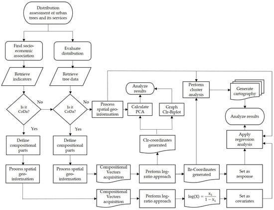
Figure 2.
Methodology flowchart.
3. Results
3.1. Assessing the Distribution of Urban Trees in Guadalajara
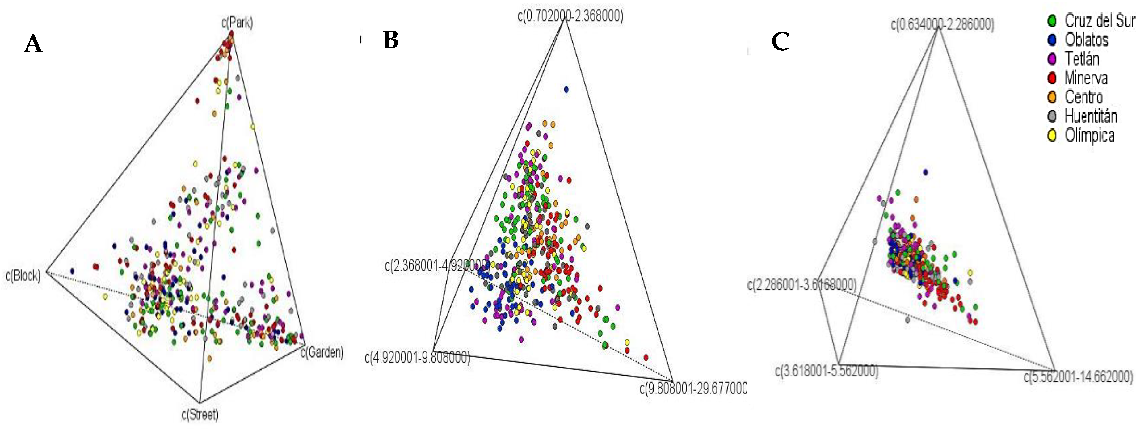
A first exploratory approach in the simplex depicts the raw data (Figure 3). The sample of the compositions given to each characteristic is shown (i.e., location type, height and diameter). Each point represents the composition of a neighborhood. The neighborhoods are color-coded by urban district, and the vertices of the tetrahedrons correspond to the different compositional parts (Figure 3).
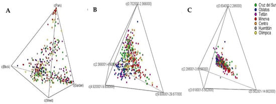
Figure 3.
Sample of compositional vectors displayed in the simplex by: (A) location type, (B) height and (C) diameter.
It is clear that the data is compositional, and that the space in which they live is the simplex (Figure 3A–C). Interpreting the relationships of the data in this space is complicated. The simplex implies a proper geometric structure with proper operations and distances. When the data is expressed as clr or ilr/olr coordinates (depending on the analysis), the coordinates lie in the Euclidian geometry, and classical statistical tools such as PCA and cluster analysis can be performed to analyze the data.
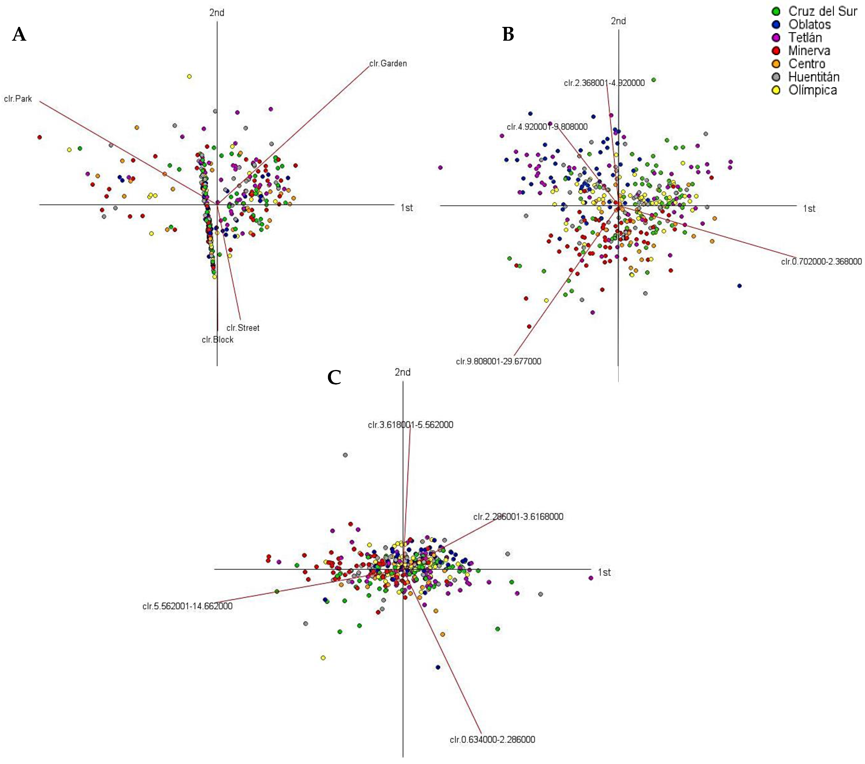
In the present study, the PCA analyses are performed on the clr-transformed data (i.e., location type, height and diameter). By location type, the total variance explained by PC1 and PC2 is 52% and 36%, respectively, with a cumulative proportion of 88%. The first two components of the analysis for the heights captured 94% of the variance. PC1 captured 58%, and PC2 captured 36%, of the total variance. Finally, PC1 and PC2 of the analysis performed for the diameters explained 79% and 14% of the total variance, respectively.
In order to better understand the variability and behavior of the observations, PCA results are depicted in clr-biplots (Figure 4), favoring the display of observations (form clr-biplot, α = 1). In Figure 4A, the main factor differentiating the neighborhoods is the opposition between clr of trees in parks with respect to the others. That is, an observation (neighborhood) with a large value of clr of trees in parks has a low value on the others, and vice versa. Additionally, the higher the clr of trees in streets, the more clr of trees in blocks of neighborhoods (Figure 4A). There is no trend in the clr-biplot of trees by location type.

Figure 4.
Clr-biplots by (A) location type, (B) height and (C) diameter.
In the clr-biplots by height and by diameter, a particular behavior is observed in the Minerva (red) and Oblatos (blue) districts, which are high-income and low-income districts, respectively. In Figure 4B,C, neighborhoods belonging to the Minerva district have a large value on the clr of Int4. In contrast, neighborhoods with the lowest clr of Int4 belong to the Oblatos district. The behavior between these districts and their neighborhoods illustrate the historical and still existing west–east dichotomy that segregates the city according to socioeconomic status, with the richer inhabitants in the west and the more deprived in the east.
3.2. Characterizing the Neighborhoods of Guadalajara
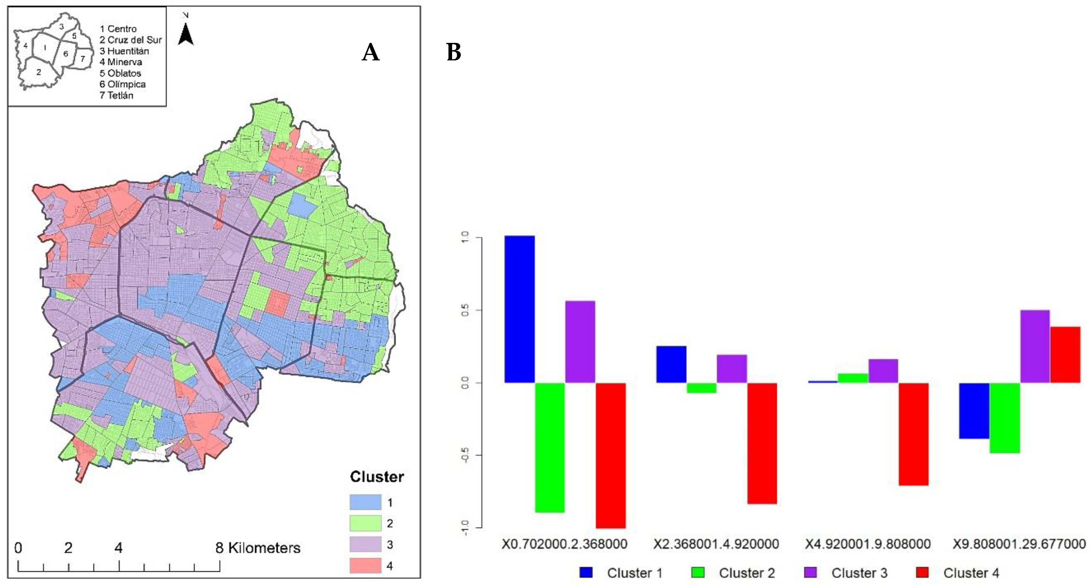
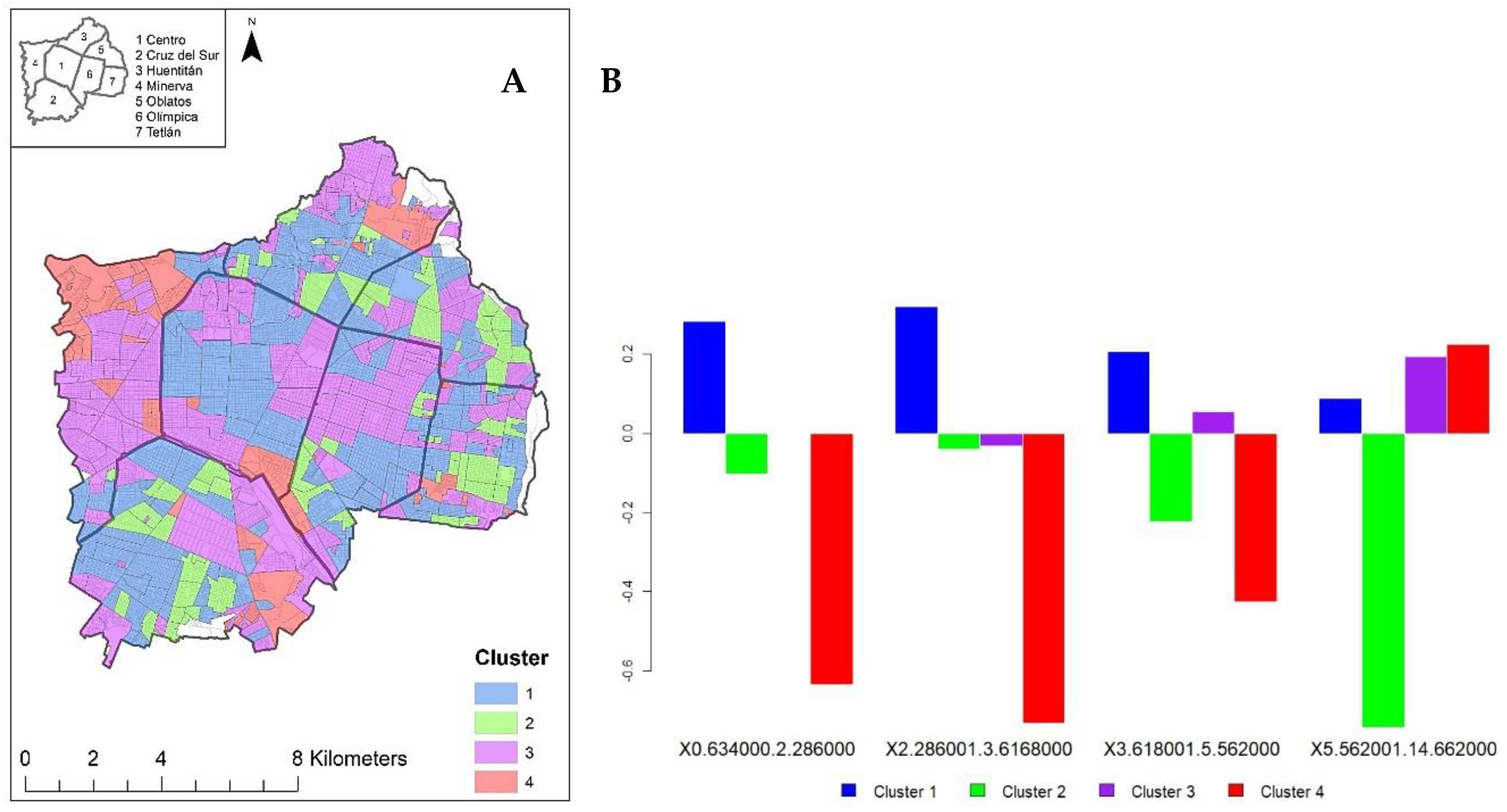
As explained in Section 2.4, the ilr/olr coordinates are used in the hierarchical cluster considering Ward’s sum of squares criterion. Four groups were selected from the dendrogram obtained in the analysis; hence, each neighborhood belongs to one of the four groups. The same procedure was performed to the different samples of compositional vectors.
Each neighborhood is shown in Figure 5A as color coded according to the cluster to which it belongs. The characteristics of each of them is shown in the geometrical mean bar plot (Figure 5B). All neighborhoods seem to be homogenous with respect to trees in the streets and trees in blocks (Figure 5), with no clear trend indicating that trees are unevenly distributed in the city.
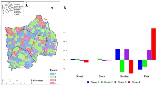
Figure 5.
Cluster analysis of trees in the city by location type. (A) Neighborhoods by cluster. (B) Cluster characterization.
However, direct observation of the territory allows us to appreciate the unreliability of these results. Once on site, the differences in the quality of urban trees between neighborhoods of different economic status are highly evident (for an example, see Figure 6). These images exemplify the differences encountered in the quality and characteristics of urban trees (i.e., height and diameter) depending on the district. Therefore, given the need to conduct a reliable and accurate analysis, the analysis was performed using the ilr/olr coordinates of trees by height and diameter.

Figure 6.
Differences in street tree characteristics. (A) Street trees in the Minerva district. (B) Street trees in the Oblatos district. Google Street View.
The cluster analysis performed to the ilr/olr coordinates of trees by height shows a clear differentiation within the city (Figure 7). In particular, most neighborhoods in the north, south and east of the city are characterized by trees of small size. In contrast, neighborhoods in the west side of the city, and particularly in the Minerva district, are characterized by with large trees, reproducing the historical spatial segregation.
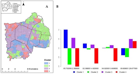
Figure 7.
Cluster analysis of trees in the city by height. (A) Neighborhoods by cluster. (B) Cluster characterization.
The analysis performed using the ilr/olr coordinates of trees by diameter (Figure 8) shows a similar trend as the one obtained from the tree heights (Figure 7). The neighborhoods of the Minerva district are characterized by trees with a larger canopy diameter as compared to the rest of the districts, while the rest of the city has trees with a small canopy diameter.
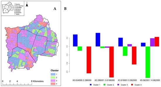
Figure 8.
Cluster analysis of trees in the city by diameter. (A) Neighborhoods by cluster. (B) Cluster characterization.
The cluster analyses performed using the ilr/olr coordinates of trees by their height and diameter are congruent with the observed reality of the city. These results highlight the existence of an unequal distribution of trees based on characteristics such as diameter and height, which suggests an unfair distribution of ecosystem services.
3.3. Who Is Benefitting from Urban Trees Ecosystem Services in Guadalajara?
As explained in Section 2.5, the ilr/olr coordinates of trees by their different attributes are used as response variables and the socioeconomic variables as independent variables (Table 4) in the regression analysis. From the different analyses, a weak predictive capacity is obtained. However, the significance of the covariates influencing the analyses was used in order to depict the association between trees and socioeconomic variables (inequity hypothesis). Interesting results were obtained by analyzing the ilr/olr coordinates of trees by location type, especially in coordinate two X*2 (Table 5). The ilr/olr balance coordinate X*2 showed a significant association between households owning a car and street trees. The same behavior was observed with households owning cell phones.

Table 5.
Regression analysis of trees by location type and socioeconomic variables.
With regard to the heights of the trees, a significant association is observed in trees of considerable height and households owning a car. The above is observed mainly in the balance coordinate X*2 model (Table 6).

Table 6.
Regression analysis of trees by height and socioeconomic variables.
Similarly, there was a significant relationship between households owning a car and trees of greater canopy diameter, particularly in the second balance coordinate X*2 (Table 7). These results indicated that higher-income residents tend to live in neighborhoods with better canopy quality, thus allowing them to benefit from trees ecosystem services.

Table 7.
Regression analysis of trees by canopy diameter and socioeconomic variables.
4. Discussion
In this study, we evaluated the distributional patterns of trees by location type, height and canopy diameter in the city of Guadalajara, Mexico. The results show an unequal distribution of trees by height and diameter within the city. Furthermore, we found an association between urban trees and households with high socioeconomic status. Similar results have been obtained by Landry and Chakraborty [44], Hernández and Villaseñor [53] and Wang and Qiu [54] in which the existence and accessibility of trees is related to high-stratum households in different urban areas.
According to the analysis, neighborhoods in high-income districts (such as Minerva) have a higher-quality tree coverage. Trees tend to be taller and have a greater canopy diameter in this district. A similar trend in the Centro district was found, although not as remarkable as in the Minerva district. The above has severe implications. The characteristics of trees (e.g., trunk, leaf size, specie, canopy diameter, height) influence the quality and the amount of ecosystem services they provide to cities [90]. In this sense, inhabitants in the Minerva district might be exposed to more environmental benefits caused by trees ecosystem services (e.g., air purification, pollution removal, runoff mitigation and temperatures regulation) than in the rest of the city, reproducing a socio-spatial segregation that has been present since the foundation of the city. Coupled with the unequal distribution of urban trees in Guadalajara, we found a significant association between trees and high socioeconomic households, and in particular, with households that own a car. In Latin American countries, car ownership is a symbol of status and purchasing power [69]. In this sense, deprived households might be more vulnerable to environmental health issues caused by the inhabitants who enjoy a better quality of life and by the environmental pressures caused by the 50% of the people who work in the city without living in it [61].
Guadalajara was founded under a clear social differentiation. The results might be due to the foundation processes coupled with changes in the urban development of the city. The San Juan de Dios River (which is currently the Independencia Causeway) served as a natural frontier that divided the city internally. The Spaniards and rich people lived to the west of the river, and the indigenous population lived to the east of the river [91]. The Spaniards established a defined urban model characterized by straight lines, ninety degree angles and wide and straight streets at the west side. In contrast, the indigenous people lived under an organic/natural model without a systematic order. Moreover, the first high-end urban and housing development models were developed in the western part of the city [91]. These new models were born with the name of colonias by the end of the 19th and the beginning of the 20th century. Such models, appealed to a discourse of modernization, had urban influences from Jorge Eugenio Haussman, in Paris; Idelfonso Cerdà, in Barcelona; and Ebenezer Howard in England [92]. These projects managed to consolidate and were characterized by green areas, wide streets and opulent households. In these new models of living, the presence of green areas was considered of great importance. Such is the case of the colonia Chapalita, in which by regulation the 40% of the total household surface was devoted to gardens [92]. In 1960 and to the west of the city, the gated communities emerged. A new way of life characterized by the exclusivity, the quality of green areas, the functionality and a closed perimeter of walls and fences. On the other hand, the urban development to the east of the city was aimed at people with low salary capacity. Small lots in physically and socially devalued spaces [92,93,94]. Furthermore, due to the emergence of the industrial capitalism in Latin America, from 1940 to 1970, the city experienced a significant population growth. In 1940, the city had a population of about 236,557 inhabitants in an area of 1994 hectares. By 1970, the city had approximately 1,529,598 inhabitants on 11,005 hectares. Between 1940 and 1970, the population of the city grew almost seven times in population and six times in area [60]. After 1970, population growth stagnated due to depletion of available land (the expansion model was mainly horizontal). The consequences of this economic model were not lived exclusively in Guadalajara and similar consequences took place in different Latin American urban contexts [95,96,97]. In addition, modifications of structural reforms in Mexico from 1982 to 1988 provoked the state to abandon its role as an urban planner, which further accentuated the west–east differences and that are currently perceived [98,99].
Accordingly, in the Centro and Minerva districts, the urban structure (such as a wider street area) can be expected to have influence in the integration of urban trees. In addition, studies have found that socioeconomic groups with a high status find the ecological and aesthetic benefits of trees more appealing [53]. On the other hand, in the eastern part of the city, the space for urban tree integration was smaller, which might have influenced its differences to the west side of the city. Additionally, during the 2010–2012 period, the city government implemented a series of projects on the east side of the city. Through the creation of public spaces (e.g., gardens, parks and public squares), the government sought to achieve socio-spatial integration, fight poverty and achieve sustainability. Nevertheless, these projects were damaged by the same inhabitants and some areas keep on presenting social problems [100]. Studies have shown that groups with low socioeconomic status tend to resist planting trees. The cost in tree maintenance (e.g., watering, pruning, pest control), the increase in land prices, rising rents and processes of gentrification, among others, are some of the reasons [39,41,101].
The results obtained in this study reveal that the city has a large number of challenges for the compliance of the SDGs by 2030, and particularly for Objectives 10 (reduced inequalities), 11 (sustainable cities and communities) and 13 (climate action). As part of the 2030 targets, the government intends to have a daily average of air quality index of 25 IMECAS (Metropolitan Air Quality Index (IMECA). Index that transforms and integrates a group of pollutants (O3, CO, SO2, NO2, PST, PM10, PM2.5) on a scale of 0 to 500 corresponding to air quality (between 0–100 as satisfactory, 101–200 as unsatisfactory, 201–300 as bad and, 301–500 asvery extremely bad)); a coverage of green areas of 9 m2/inhabitant; 100% of the population satisfied with the public space offered by the city; gardens and parks with no signs of deterioration; an intensive urban reforestation with a 90% rate of new urban trees in comparison with the previous year and finally a response rate of 24 h in citizen reports on incidents [61]. However, the daily air quality index in the city is on average of 48 IMECAS. Approximately 34% of the population live in areas with poor coverage of green areas (less than 4 m2/inhabitant). Likewise, nearly 50% of parks, gardens and public spaces are in poor conditions, and only 81% of citizens reporting on incidents in these spaces are resolved, with an average response time of 60 days [61]. Of the urban trees, 77% require some type of intervention (e.g., fertilization, pest control, demolition of dry trees, etc.). Furthermore, the city has a weak tax collection capacity that affects the maintenance and provision of public space. The adoption of SDGs in urban policies are a good opportunity to improve both green infrastructure planning as well as the distribution of ecosystem services among the inhabitants. Nevertheless, the actions carried out in Guadalajara to date appear to be insufficient and have had no impact, as the results have explained.
According to public information of the Public Works department of the city, only three projects (Projects DOP-REH-MUN-JAR-LP-008-16, DOP-REH-MUN-JAR-LP-009-16 and DOP-REH-MUN-JAR-LP-010-16) included the word “trees” in 2016. In these contracts, the government of the municipality focused on the rehabilitation of urban trees in the Centro district. The federal and state government performed five and one project, respectively, involving trees in the east part of the city (Projects DOP-CON-FED-PDR-CI-168-16, DOP-CON-FED-PDR-LP-136-16, DOP-CON-FED-PDR-LP-137-16, DOP-CON-FED-PDR-LP-138-16, DOP-CON-FED-PDR-LP-139-16 and DOP-REH-EST-MER-CI-257-16). There is no information on the number of trees, the species or the criteria for selecting the areas where they were planted. Thus, it seems that an environmental justice approach has not been adopted in the allocation of trees in the city. Since 2016, no public works related to urban trees have been found.
It is important to highlight that with a greater availability of information in this first (and only) census of trees conducted by the city government, and applying the same methodology, the results would have been enriched. Nevertheless it has been mentioned that the canopy diameter and the height influence in the quality of the ecosystem services provided [90], having the species of each tree in the census would have allowed a better analysis. In consequence, the event of execution of a census that includes more variables, such as tree species, would make it possible to perform the analysis with specific ecosystem services. With this information, plus the use of tools such as the i-Tree Eco software, the ecosystem services provided by each tree (e.g., NO2, SO2, O3, CO and PM2.5 removal), can be obtained. In this sense, the compositional vectors (previously defined as neighborhoods) would be formed by different parts (ecosystem services).
Additionally, in the future, it would be interesting to analyze the processes of green gentrification in the city. In other words, the objective is to analyze whether different neighborhoods suffer changes in the sociodemographic characteristics of their inhabitants and as for an increase in the land cost caused by the amount of greenery in the said neighborhood.
5. Conclusions
In this study, the distribution of trees in Guadalajara was evaluated using compositional data analysis. Through PCA and cluster analyses, we found a clear differentiation in the distribution of trees between the west and east of the city. Furthermore, through regression analysis, a significant relationship is found between households owning a car and street trees, tall trees and trees with a large canopy diameter. This highlights the existence of an environmental injustice that falls directly on deprived households and neighborhoods. High strata inhabitants are favored with the ecosystem services provide by urban trees in Guadalajara. The uneven distribution of urban trees in the city of Guadalajara might be a consequence of either or both of two factors: (i) the different social and economic forces that date back to the foundation of the city, and that have been reinforced until the present day, and (ii) the weak urban policies to transform SDGs integration and environmental justice perspective into plans and actions that are actually performed. Finally, we would like to stress that the method used in this study is applicable to any urban context and for the study of any other urban phenomena.
Author Contributions
Conceptualization, M.C.-S., M.I.O., and E.R.; methodology, M.I.O.; formal analysis, M.C.-S., M.I.O., and E.R.; investigation, M.C.-S.; data curation, M.C.-S.; writing—original draft preparation, M.C.-S.; writing—review and editing, M.C.-S., M.I.O., and E.R.; supervision, M.I.O. and E.R. All authors have read and agreed to the published version of the manuscript.
Funding
This work was developed in the framework of a grant received by the Mexican government through a CONACYT fellowship (Reference 612800) and partially supported by grants RTI2018-095518-B-C22 and PCI2019-103674 (MCIU/AEI/FEDER) of the Spanish Ministry of Science, Innovation and Universities, and the European Regional Development Fund.
Conflicts of Interest
The authors declare no conflict of interest.
References
- Greenwalt, J.; Raasakka, N.; Alverson, K. Building Urban Resilience to Address Urbanization and Climate Change. In Resilience; Zommers, Z., Alverson, K., Eds.; Elsevier Inc.: Amsterdam, The Netherlands, 2018; pp. 151–164. ISBN 9780128118917. [Google Scholar]
- Liang, L.; Wang, Z.; Li, J. The effect of urbanization on environmental pollution in rapidly developing urban agglomerations. J. Clean. Prod. 2019, 237, 117649. [Google Scholar] [CrossRef]
- Grimm, N.B.; Faeth, S.H.; Golubiewski, N.E.; Redman, C.L.; Wu, J.; Bai, X.; Briggs, J.M. Global change and the ecology of cities. Science 2008, 319, 756–760. [Google Scholar] [CrossRef] [PubMed]
- Cai, W.; Liu, C.; Zhang, C.; Ma, M.; Rao, W.; Li, W.; He, K.; Gao, M. Developing the ecological compensation criterion of industrial solid waste based on emergy for sustainable development. Energy 2018, 157, 940–948. [Google Scholar] [CrossRef]
- Rahmasary, A.N.; Robert, S.; Chang, I.S.; Jing, W.; Park, J.; Bluemling, B.; Koop, S.; van Leeuwen, K. Overcoming the Challenges of Water, Waste and Climate Change in Asian Cities. Environ. Manage. 2019, 63, 520–535. [Google Scholar] [CrossRef]
- Nedved, M.; Jansz, J. Waste water pollution control in the Australian mining industry. J. Clean. Prod. 2006, 14, 1118–1120. [Google Scholar] [CrossRef]
- Hassan Rashid, M.A.U.; Manzoor, M.M.; Mukhtar, S. Urbanization and its effects on water resources: An exploratory analysis. Asian J. Water, Environ. Pollut. 2018, 15, 67–74. [Google Scholar] [CrossRef]
- Lin, B.; Zhu, J. Changes in urban air quality during urbanization in China. J. Clean. Prod. 2018, 188, 312–321. [Google Scholar] [CrossRef]
- Ponce, P.; Alvarado, R. Air pollution, output, FDI, trade openness, and urbanization: Evidence using DOLS and PDOLS cointegration techniques and causality. Environ. Sci. Pollut. Res. 2019, 26, 19843–19858. [Google Scholar] [CrossRef]
- Hodgkins, G.A.; Dudley, R.W.; Archfield, S.A.; Renard, B. Effects of climate, regulation, and urbanization on historical flood trends in the United States. J. Hydrol. 2019, 573, 697–709. [Google Scholar] [CrossRef]
- Huang, G. A Revisit to Impact of Urbanization on Flooding. In Urban Planning and Water-Related Disaster Management; Huang, G., Shen, Z., Eds.; Springer: Cham, Germany; pp. 43–56. ISBN 978-3-319-90172-5.
- Li, G.; Zhang, X.; Mirzaei, P.A.; Zhang, J.; Zhao, Z. Urban heat island effect of a typical valley city in China: Responds to the global warming and rapid urbanization. Sustain. Cities Soc. 2018, 38, 736–745. [Google Scholar] [CrossRef]
- Goddard, I.L.M.; Tett, S.F.B. How much has urbanisation affected United Kingdom temperatures? Atmos. Sci. Lett. 2019, 20, 1–6. [Google Scholar] [CrossRef]
- Lafortezza, R.; Sanesi, G. Nature-based solutions: Settling the issue of sustainable urbanization. Environ. Res. 2019, 394–398. [Google Scholar] [CrossRef] [PubMed]
- Wei, J.; Qian, J.; Tao, Y.; Hu, F.; Ou, W. Evaluating spatial priority of urban green infrastructure for urban sustainability in areas of rapid urbanization: A case study of Pukou in China. Sustainability 2018, 10, 327. [Google Scholar] [CrossRef]
- United Nations Sustainable Development Goals. Available online: https://sustainabledevelopment.un.org/?menu=1300 (accessed on 5 July 2019).
- De Sousa, S.; Panagopoulos, T. Environmental Justice in Accessibility to Green. Land 2018, 7, 1–23. [Google Scholar]
- Wolch, J.R.; Byrne, J.; Newell, J.P. Urban green space, public health, and environmental justice: The challenge of making cities ‘just green enough’. Landsc. Urban Plan. 2014, 125, 234–244. [Google Scholar] [CrossRef]
- Cole, H.V.S.; Triguero-mas, M.; Connolly, J.J.T.; Anguelovski, I. Determining the health bene fi ts of green space: Does gentri fi cation matter? Health Place 2019, 57, 1–11. [Google Scholar] [CrossRef]
- Russo, A.; J Escobedo, F.; Zerbe, S. Quantifying the local-scale ecosystem services provided by urban treed streetscapes in Bolzano, Italy. AIMS Environ. Sci. 2016, 3, 58–76. [Google Scholar] [CrossRef]
- Ziter, C.D.; Pedersen, E.J.; Kucharik, C.J.; Turner, M.G. Scale-dependent interactions between tree canopy cover and impervious surfaces reduce daytime urban heat during summer. Proc. Natl. Acad. Sci. USA 2019, 1–6. [Google Scholar] [CrossRef]
- Duncan, J.M.A.; Boruff, B.; Saunders, A.; Sun, Q.; Hurley, J.; Amati, M. Science of the Total Environment Turning down the heat: An enhanced understanding of the relationship between urban vegetation and surface temperature at the city scale. Sci. Total Environ. 2019, 656, 118–128. [Google Scholar] [CrossRef]
- Zhang, B.; Xie, G.; Zhang, C.; Zhang, J. The economic benefits of rainwater-runoff reduction by urban green spaces: A case study in Beijing, China. J. Environ. Manage. 2012, 100, 65–71. [Google Scholar] [CrossRef]
- Oke, T.R.; Crowther, J.M.; Mcnaughton, K.G.; Monteith, J.L.; Gardiner, B. The Micrometeorology of the Urban Forest [ and Discussion ]. Philos. Trans. R. Soc. B 1989, 324, 335–349. [Google Scholar]
- Kercher, G.J. Anglin 22 Benefits of Urban Street Trees. Available online: https://www.pleasanthilliowa.org/DocumentCenter/View/511/22-Benefits-of-Urban-Street-Trees?bidId= (accessed on 20 July 2019).
- De Carvalho, R.M.; Szlafsztein, C.F. Urban vegetation loss and ecosystem services: The influence on climate regulation and noise and air pollution. Environ. Pollut. 2019. [Google Scholar] [CrossRef] [PubMed]
- Guo, T.; Morgenroth, J.; Conway, T. To plant, remove, or retain: Understanding property owner decisions about trees during redevelopment. Landsc. Urban Plan. 2019, 190, 103601. [Google Scholar] [CrossRef]
- Sander, H.; Polasky, S.; Haight, R.G. The value of urban tree cover: A hedonic property price model in Ramsey and Dakota. Ecol. Econ. 2010, 69, 1646–1656. [Google Scholar] [CrossRef]
- Burley, B.A. Green infrastructure and violence: Do new street trees mitigate violent crime? Health Place 2018, 54, 43–49. [Google Scholar] [CrossRef]
- Wolf, K.L. Freeway roadside management: The urban forest beyond the white line. J. Arboric. 2003, 29, 127–136. [Google Scholar]
- Wolf, K.L. Business District Streetscapes, Trees, and Consumer Response. J. For. 2001, 103, 396–400. [Google Scholar]
- Kweon, B.; Sullivan, W.C.; Wiley, A.R. Green common spaces and the social integration of inner-city older adults. Environ. Behav. 1998, 832–858. [Google Scholar] [CrossRef]
- Takano, T.; Nakamura, K.; Watanabe, M. Urban residential environments and senior citizens’ longevity in megacity areas: The importance of walkable green spaces. J. Epidemiol. Community Health 2002. [Google Scholar] [CrossRef]
- Kardan, O.; Gozdyra, P.; Misic, B.; Moola, F.; Palmer, L.J.; Paus, T. Neighborhood greenspace and health in a large urban center. Sci. Rep. 2015, 5, 11610. [Google Scholar] [CrossRef]
- Anguelovski, I.; Connolly, J.J.T.; Masip, L.; Pearsall, H.; Anguelovski, I.; Connolly, J.J.T.; Masip, L.; Pearsall, H.; Anguelovski, I. Assessing green gentrification in historically disenfranchised neighborhoods: A longitudinal and spatial analysis of Barcelona Barcelona. Urban Geogr. 2017, 39, 458–491. [Google Scholar] [CrossRef]
- Gould, K.A.; Lewis, T.L. Green Gentrification. Urban Sustainability and the Struggle for Environmental Justice, 1st ed.; Agyeman, J., Patel, Z., Eds.; Routledge.Taylor & Francis Group: New York, NY, USA, 2017; ISBN 978-1-138-92016-3. [Google Scholar]
- Anguelovski, I.; Irazábal-Zurita, C.; Connolly, J.J.T. Grabbed Urban Landscapes: Socio-spatial Tensions in Green Infrastructure Planning in Medellín. Int. J. Urban Reg. Res. 2019, 43, 133–156. [Google Scholar] [CrossRef]
- Checker, M. Wiped Out by the “Greenwave”: Environmental Gentrification and the Paradoxical Politics of Urban Sustainability. City Soc. 2011, 23, 210–229. [Google Scholar] [CrossRef]
- Schwarz, K.; Fragkias, M.; Boone, C.G.; Zhou, W.; McHale, M.; Grove, J.M.; O’Neil-Dunne, J.; McFadden, J.P.; Buckley, G.L.; Childers, D.; et al. Trees grow on money: Urban tree canopy cover and environmental justice. PLoS ONE 2015, 10, e0122051. [Google Scholar] [CrossRef]
- Byrne, J.; Wolch, J. Nature, race, and parks: Past research and future directions for geographic research. Prog. Hum. Geogr. 2009, 33, 743–765. [Google Scholar] [CrossRef]
- Carmichael, C.E.; McDonough, M.H. Community Stories: Explaining Resistance to Street Tree-Planting Programs in Detroit, Michigan, USA. Soc. Nat. Resour. 2019, 32, 588–605. [Google Scholar] [CrossRef]
- Baró, F.; Calderón-Argelich, A.; Langemeyer, J.; Connolly, J.J.T. Under one canopy? Assessing the distributional environmental justice implications of street tree benefits in Barcelona. Environ. Sci. Policy 2019, 102, 54–64. [Google Scholar] [CrossRef]
- Park, Y.M.; Kwan, M.P. Multi-contextual segregation and environmental justice research: Toward fine-scale spatiotemporal approaches. Int. J. Environ. Res. Public Health 2017, 14, 1205. [Google Scholar]
- Landry, S.M.; Chakraborty, J. Street trees and equity: Evaluating the spatial distribution of an urban amenity. Environ. Plan. 2009, 41, 2651–2671. [Google Scholar] [CrossRef]
- Maroko, A.R.; Maantay, J.A.; Sohler, N.L.; Grady, K.L.; Arno, P.S. The complexities of measuring access to parks and physical activity sites in New York City: A quantitative and qualitative approach. Int. J. Health Geogr. 2009, 23, 1–23. [Google Scholar] [CrossRef]
- Coen, S.E.; Ross, N.A. Exploring the material basis for health: Characteristics of parks in Montreal neighborhoods with contrasting health outcomes. Health Place 2006, 12, 361–371. [Google Scholar] [CrossRef] [PubMed]
- Lewis, T.L. Global Civil Society and the distribution of environmental goods: Funding for environmental NGO’s in Ecuador. In Inequalities, Environmental Beyond Borders. Local Perspectives on Global Injustices; Joann, C., Agyeman, J., Eds.; The MIT Press: Cambridge, MA, USA, 2011; pp. 88–104. ISBN 9780262015516. [Google Scholar]
- Gould, K.A.; Lewis, T.L. From Green Gentrification to Resilience Gentrification: An Example from Brooklyn 1. City Community 2018, 12–15. [Google Scholar] [CrossRef]
- Scopelliti, M.; Carrus, G.; Adinolfi, C.; Suarez, G.; Colangelo, G.; Lafortezza, R. Staying in touch with nature and well-being in different income groups: The experience of urban parks in Bogotá. Landsc. Urban PLa 2016, 148, 139–148. [Google Scholar] [CrossRef]
- Zhou, X.; Kim, J. Social disparities in tree canopy and park accessibility: A case study of six cities in Illinois using GIS and remote sensing. Urban For. Urban Green. 2013, 12, 88–97. [Google Scholar] [CrossRef]
- Chuang, W.-C.; Boone, C.G.; Locke, D.H.; Grove, J.M.; Whitmer, A.L.; Geoffrey, B.; Zhang, S. Tree canopy Change and neighborhood stability: A Comparative Analysis of Washington, DC and Baltimore, MD. Urban For. Urban Green. 2017, 27, 363–372. [Google Scholar] [CrossRef]
- Krafft, J.; Fryd, O. Spatiotemporal patterns of tree canopy cover and socioeconomics in Melbourne. Urban For. Urban Green. 2016, 15, 45–52. [Google Scholar] [CrossRef]
- Hernández, H.J.; Villaseñor, N.R. Twelve-year change in tree diversity and spatial segregation in the Mediterranean city of Santiago, Chile. Urban For. Urban Green. 2018, 29, 10–18. [Google Scholar] [CrossRef]
- Wang, H.; Qiu, F. Spatial disparities in neighborhood public tree coverage: Do modes of transportation matter? Urban For. Urban Green. 2018, 29, 58–67. [Google Scholar] [CrossRef]
- Cole, H.V.S.; Lamarca, M.G.; Connolly, J.J.T.; Anguelovski, I.; Hospital, I. Are green cities healthy and equitable? Unpacking the relationship between health, green space and gentrification. Epidemiol Community Heal. 2017, 71, 1118–1121. [Google Scholar] [CrossRef]
- Mills, J.R.; Cunningham, P.; Donovan, G.H. Urban forests and social inequality in the Pacific Northwest. Urban For. Urban Green. 2016, 16, 188–196. [Google Scholar] [CrossRef]
- Pawlowsky-Glahn, V.; Egozcue, J.J. Compositional data and their analysis: An introduction. In Compositional Data Anlaysis in the Geosciences. From Theory to Practice; Buccianti, A., Mateu-Figueras, G., Paw, Eds.; The Geological Society: London, UK, 2006; pp. 1–10. ISBN 1-86239-205-6. [Google Scholar]
- Filzmoser, P.; Hron, K.; Templ, M. Applied Compositional Data Analysis, 1st ed.; Diggle, P., Gather Ursula, Z.S., Eds.; Springer Series in Statistics: Cham, Switzerland, 2018; ISBN 978-3-319-96420-1. [Google Scholar]
- Marcillo-Delgado, J.C.; Ortego, M.I.; Pérez-Foguet, A. A compositional approach for modelling SDG7 indicators: Case study applied to electricity access. Renew. Sustain. Energy Rev. 2019, 107, 388–398. [Google Scholar] [CrossRef]
- IMEPLAN. Area metropolitana de Guadalajara, Expansión urbana, Análisis y prospectiva: 1970–2045, 1st ed.; Orozco, A., Shalisko, V., Rodríguez, M., Hernández, D., Morfín, J., Chávez, R., Eds.; Editoriales e Industrias Creativas de México SA de CV: Guadalajara, Mexico, 2015; Volume 1. [Google Scholar]
- Government of Guadalajara. Plan Municipal de Desarrollo y Gobernanza 2018–2021; Government of Guadalajara: Guadalajara, Mexico, 2018.
- Government of Guadalajara. Plan Municipal de Desarrollo Guadalajara 2015–2018, 500 Visión 2042; Government of Guadalajara: Guadalajara, Mexico, 2016; Volume II.
- Government of Guadalajara. Online Mapping Service of the Government of Guadalajara. Available online: https://mapa.guadalajara.gob.mx/ (accessed on 1 May 2019).
- ESRI ArcMap, version 10.2.2, ArcGIS Desktop. Eris: Redlands, CA, USA, 2013.
- ESRI Natural Ruptures (Jenks). Available online: https://pro.arcgis.com/es/pro-app/help/mapping/layer-properties/data-classification-methods.htm (accessed on 1 August 2019).
- Government of Guadalajara GeoGDL. Available online: https://mapa.guadalajara.gob.mx/geomap (accessed on 5 June 2019).
- INEGI Cartografía geoestadística urbana, Cierre del Censo de Población y Vivienda 2010. Guadalajara. Available online: https://www.inegi.org.mx/app/biblioteca/ficha.html?upc=702825588335 (accessed on 25 January 2020).
- INEGI Sistema para la Consulta de Información Censal 2010. Available online: http://gaia.inegi.org.mx/scince2/viewer.html (accessed on 1 May 2019).
- UN-Habitat. Planning and Design for Sustainable Urban Mobility. Global Report on Human Settlements, 1st ed.; Routledge: Abingdon, UK, 2013; ISBN 9780415723183. [Google Scholar]
- INEGI Principales resultados por AGEB y manzana urbana. Instituto Nacional de Estadística Geografía e Informática. Censo Población y Vivienda 2010, 1–19.
- R Core Team. R: A Language and Environment for Statistical Computing; R Foundation for Statistical Computing: Vienna, Austria, 2014. [Google Scholar]
- RStudio Team. RStudio: Integrated Development Environment for R; R Foundation for Statistical Computing: Vienna, Austria, 2016. [Google Scholar]
- Comas-Cufí, M.; Thió-Henestrosa, S. CoDaPack 2.0: A stand-alone, multi-platform compositional software. In Proceedings of the CoDaWork’11: 4th International Workshop on Compositional Data Analysis, Sant Feliu de Guíxols, Spain, 9–13 May 2011. [Google Scholar]
- Egozcue, J.J. Reply to “On the Harker vriation diagrams;...” by J.A. Cortés. Math. Geosci. 2009, 41, 829–834. [Google Scholar] [CrossRef]
- Pawlowsky-Glahn, V.; Egozcue, J.J.; Tolosana-Delgado, R. Modeling and Analysis of Compositional Data, 1st ed.; John Wiley & Sons: London, UK, 2015; ISBN 9783540773405. [Google Scholar]
- Pearson, K. Mathematical Contributions to the Theory of Evolution.—On a Form of Spurious Correlation Which May Arise When Indices Are Used in the Measurement of Organs. Proc. R. Soc. London 1896, 60, 489–498. [Google Scholar]
- Chayes, F. Ratio Correlation: A Manual for Students of Petrology and Geochemistry; University of Chicago Press: Chicago, IL, USA, 1971. [Google Scholar]
- Aitchison, J. The Statistical Analysis of Geochemical Compositions. Math. Geol. 1984, 16, 15–18. [Google Scholar] [CrossRef]
- Aitchison, J. The Statistical Analysis of Compositional Data. Monographs on Satistics and Applied Probability, Chapman & Hall Ltd, Ed.; 1st ed.; Springer: London, UK, 1986; ISBN 978-0412280603. [Google Scholar]
- Rock, N.M.S. Lecture Notes in Earth Sciences; Bhattacharji, S., Friedmand, G.M., Neugebauer, H.J., SeilacherAdolf, Eds.; Springer-Verlag New York Inc.: Nedlands, Western Australia, 1988. [Google Scholar]
- Rollinson, H.R. Another look at the constant sum problem in geochemistry. Mineral. Mag. 1992, 56, 469–475. [Google Scholar] [CrossRef]
- Martín-Fernández, J.A.; Palarea-Albaladejo, J.; Olea, R.A. Dealing with Zeros. In Compositional Data Anlaysis: Theory and Applications; Pawlowsky-Glahn, V., Buccianti, A., Eds.; Wiley: Hoboken, NJ, USA, 2011; pp. 43–58. [Google Scholar]
- Egozcue, J.J.; Pawlowsky-Glahn, V.; Mateu-Figueras, G.; Barceló-Vidal, C. Isometric Logratio Transformations for Compositional Data Analysis. Math. Geol. 2003, 35, 279–300. [Google Scholar] [CrossRef]
- O’Sullivan, D.; Unwin, D. Reducing the number of variables: Principal Component Analysis. In Geographic Information Analysis; John Wiley & Sons, Ed.; Wiley: Hoboken, NJ, USA, 2002; pp. 343–355. ISBN 0471211761, 9780471211761. [Google Scholar]
- Gabriel, K.R. The Biplot Graphic Display of Matrices with application to Principal Component Analysis. Biometrika 1971, 58, 453–467. [Google Scholar] [CrossRef]
- Aitchison, J. The one-hour course in compositional data analysis or compositional data analysis is simple. In Proceedings of the IAMG’97—The 3rd Annual Conference of the International Association for Mathematical Geology, Barcelona, Spain, 22–27 September 1997. [Google Scholar]
- Daunis-i-Estadella, J.; Thió-Henestrosa, S.; Mateu-Figueras, G. Computers & Geosciences Including supplementary elements in a compositional biplot. Comput. Geosci. 2011, 37, 696–701. [Google Scholar]
- Murtagh, F.; Legendre, P. Ward’s Hierarchical Agglomerative Clustering Method: Which Algorithms Implement Ward’s Criterion? J. Classif. 2014, 31, 274–295. [Google Scholar] [CrossRef]
- Egozcue, J.J.; Pawlowsky-Glahn, V. Groups of Parts and Their Balances in Compositional Data Analysis. Math. Geol. 2005, 37, 795–828. [Google Scholar] [CrossRef]
- Roy, S.; Byrne, J.; Pickering, C. A systematic quantitative review of urban tree benefits, costs, and assessment methods across cities in different climatic zones. Urban For. Urban Green. 2012, 11, 351–363. [Google Scholar] [CrossRef]
- López, E. La cuadrícula en el desarrollo de la ciudad hispanoamericana. Guadalajara, México; Universidad de Guadalajara. Instituto Tecnológico y de Estudios Superiores de Occidente: Guadalajara, Mexico, 2001. [Google Scholar]
- Cabrales, L.F.; Canosa, E. Segregación residencial y fragmentación urbana: Los fraccionamientos cerrados en Guadalajara. Espiral 2001, VII, 223–253. [Google Scholar] [CrossRef]
- Brandis-García, D.; Mas-Hernández, R. Propiedad inmueble, morfología urbana y precios del suelo en Guadalajara (siglo XIX). Tiempos de América 1997, 1, 57–69. [Google Scholar]
- Cabrales, L.F.; Chong, M.A. Divide y venderás: Promoción inmobiliaria del barrio de Artesanos de Guadalajara, 1898–1908. Scr. Nov. Rev. Electrónica Geogr. y Ciencias Soc. 2006, X, 741–798. [Google Scholar]
- Aguilar, A.G.; Escamilla, I.H. Segregación urbana y espacios de exclusión. Ejemplos de México y América Latina; Universidad Nacional Autónoma de México, UNAM. MAPorrúa: Mexico City, Mexico, 2015; ISBN 978-607-401-963-6. [Google Scholar]
- Cobos, E.P. La ciudad capitalista en el patrón neoliberal de acumulación en América Latina TT—The capitalist city in the neoliberal pattern of accumulation in Latin America. Cad. Metrópole 2014, 16, 37–60. [Google Scholar] [CrossRef]
- Guevara, T. Abordajes teóricos sobre las transformaciones sociales, económicas y territoriales en las ciudades latinoamericanas contemporáneas. Eure 2015, 41, 5–24. [Google Scholar] [CrossRef]
- Marrufo, R.M.; Bass, S. Segregación socioespacial y servicios de salud en Ciudad Juáres. In Segregación Urbana y Espacios de Exclusión; Ejemplos de México y América Latina; Aguilar, A.G., Escamilla, H.I., Eds.; Universidad Nacional Autónoma de México.Miguel Ángel Porrúa: Mexico City, Mexico, 2015; pp. 139–162. [Google Scholar]
- Moreno, O. Insustentabilidad de la vida, segregación social y pobreza urbana: Efectos de las políticas de vivienda en la era del ultraliberalismo. In Segregación Urbana y Espacios de Exclusión; Ejemplos de México y América Latina; Aguilar, A.G., Escamilla, H.I., Eds.; Universidad Nacional Autónoma de México.Miguel Ángel Porrúa: Mexico City, Mexico, 2015; pp. 307–328. [Google Scholar]
- González-Rodriguez, S.M. Las políticas urbanas de inclusión socio-espacial de la zona nor-oriente de la ciudad de Guadalajara, algunas reflexiones. Periodo 2010–2012. In Proceedings of the International Conference Virtual City and Territory. "9° Congresso Città e Territorio Virtuale, Rome, Italy, 2–4 October 2013; pp. 1470–1484. [Google Scholar]
- Danford, R.S.; Strohbach, M.W.; Ryan, R.; Nicolson, C.; Warren, P.S. What does it take to achieve equitable urban tree canopy distribution? A Boston case study. Cities Environ. 2014, 7, 1–20. [Google Scholar]
© 2020 by the authors. Licensee MDPI, Basel, Switzerland. This article is an open access article distributed under the terms and conditions of the Creative Commons Attribution (CC BY) license (http://creativecommons.org/licenses/by/4.0/).


