Abstract
Investigating the spatial and vertical patterns of wetland soil organic carbon concentration (SOCc) is important for understanding the regional carbon cycle and managing the wetland ecosystem. By integrating 160 wetland soil profile samples and environmental variables from climatic, topographical, and remote sensing data, we spatially predicted the SOCc of wetlands in China’s Western Songnen Plain by comparing four algorithms: random forest (RF), support vector machine (SVM) for regression, inverse distance weighted (IDW), and ordinary kriging (OK). The predicted results of the SOCc from the different algorithms were validated against independent testing samples according to the mean error, root mean squared error, and correlation coefficient. The results show that the measured SOCc values at depths of 0–30, 30–60, and 60–100 cm were 15.28, 7.57, and 5.22 g·kg−1, respectively. An assessment revealed that the RF algorithm was the most accurate for predicting SOCc; its correlation coefficients at the different depths were 0.82, 0.59, and 0.51, respectively. The attribute importance from the RF indicates that environmental variables have various effects on the SOCc at different depths. The land surface temperature and land surface water index had a stronger influence on the spatial distribution of SOCc at the depths of 0–30 and 30–60 cm, whereas topographic factors, such as altitude, had a stronger influence within 60–100 cm. The predicted SOCc of each vertical depth increased gradually from south to north in the study area. This research provides an important case study for predicting SOCc, including selecting factors and algorithms, and helps understanding the carbon cycles of regional wetlands.
1. Introduction
As an important carbon pool in the earth’s surface system, wetlands store 20% to 30% of the world’s carbon in the soil [1], playing a key role in the global carbon cycle [2,3]. Carbon accumulation in wetlands and emissions of wetlands have become a concerning issue for governments and academics around the world [4]. Predicting the spatial distribution of the soil organic carbon concentration (SOCc) in wetlands and studying the influencing factors are important to understand regional climate change and the wetland carbon cycle.
The spatial distribution of SOCc is affected by many factors. For example, multiple environmental variables including soil properties, climate, and terrain have important impacts on the spatial distribution of SOCc [5,6,7]. In addition to environmental factors, soil organic carbon is also affected by the soil microbial community and soil-dwelling arthropods [8,9,10]. In China’s Loess Plateau, lower temperatures and higher precipitation are beneficial for the accumulation of organic carbon [11]. In the Basque Country (northern Spain), temperature is the main climatic factor affecting the SOCc [12]. In the zonal soils of China, surface soil organic matter concentration is generally negatively correlated with the mean annual temperature (MAT) and positively correlated with the mean annual precipitation (MAP) and altitude (H) [13]. Different environmental conditions have different effects on SOCc.
Wetland carbon research is mainly limited by the research methods and data availability. Studies revealed that the prediction techniques for soil attributes are based mainly on spatial correlation, including autocorrelation and mutual correlation [14]. Commonly used autocorrelation technologies include inverse distance weighting (IDW) and ordinary kriging (OK) [15]. Spatial mutual-correlation-based predictions integrate field observations and environmental variables through quantitative relationships [16]. The main techniques for mutual-correlation-based predictions include parametric and nonparametric methods. Because the correlation of parametric methods is linear and cannot represent complex relationships [17], the nonparametric method is widely used in technologies such as artificial neural networks (ANNs) [18,19,20], support vector machine (SVM) for regression [21,22], boosted regression trees [23], and random forest (RF) [24,25,26]. Machine learning techniques have advantages over parametric methods on modeling spatially non-linear relationships [27], thus improving the prediction accuracy of spatial algorithms. Therefore, in this study, we aimed to evaluate and compare the performance of the RF, SVM, IDW, and OK algorithms for predicting SOCc.
Many wetlands are found in China’s Western Songnen Plain [28]. Due to intensive agricultural activities and clear climate change, the environment and wetlands in this area have been degraded. To deeply understand the regional carbon cycle and provide theoretical guidance for wetland management, the aims of this study were to (1) compare different algorithms (RF, SVM, IDW, and OK) and select the optimal approach; (2) explore the influence of different factors on wetland SOCc; and (3) reveal the spatial patterns of wetland SOCc in the Western Songnen Plain.
2. Materials and Methods
2.1. Study Area
The Western Songnen Plain (121°36′–126°36′ E, 43°59′–46°18′ N) is located in the central part of northeast China in a transitional zone between agricultural and pastoral regions (Figure 1). This region covers an area of 1.01 × 10⁵ km2, with an altitude from 110 to 140 m. The study area has a continental monsoon climate. The temperature increases from north to south, with an average annual value of 2–7 °C. Annual precipitation decreases from 420–550 mm in the east to 350–420 mm in the west. Precipitation varies considerably, with 70–80% of the total precipitation occurring between June and August. Dominant soil types are meadow soil, chestnut soil, and aeolian soil [29]. This region is one of the important areas of wetland distribution and has many national wetland nature reserves, such as Zhalong, Xianghai, Momoge, and Chagan Lakes [30,31]. Major native wetland plants include Reed (Phragmites australis), Cattail (Typha orientalis), and Water caltrop (Potamogeton crispus).
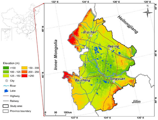
Figure 1.
Location of the Western Songnen Plain in China.
2.2. Soil Observations
The field survey was conducted from September to October 2017. Collecting soil profile samples during this time is advantageous because the soil of the wetlands has not yet frozen, and the moisture content is relatively low during these months [30]. Before the field survey, we established some sampling sites based on the wetland distribution dataset [30]. Considering the uniformity, accessibility, and the economy of the field sampling sites, 160 sampling sites were selected (Figure 2). Three different soil samples were drilled for each sampling site. Each soil sampling site included 3 soil depths: 0–30, 30–60, and 60–100 cm [32]. The SOCc of each sample at different depths was averaged from these three repeated soil samples. In this study, the SOCc was determined by the potassium dichromate external heating oxidation method [2]. The soil sample was heated with potassium dichromate in order to oxidize carbon from organic matter to carbon dioxide, and then dichromate ions were reduced. According to the change of the amount of dichromate ions by the oxidization of carbon, the SOCc can be calculated.
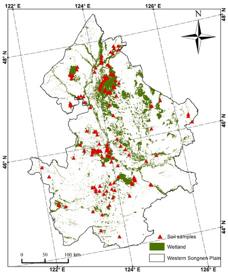
Figure 2.
Distribution of the sampling points and wetlands in the Western Songnen Plain.
2.3. Environmental Variables
The variability of SOCc could be explained by its relationships with soil-forming factors, including climate, terrain, soil properties, parent materials, and organisms. Based on data accessibility, we retrieved 30 environmental variables from the soil terrain, climate, and remote sensing data (Table 1).

Table 1.
Environmental variables for soil organic carbon concentration (SOCc) mapping.
According to meteorological data recorded during 2008–2017, the MAP (mm), MAT (°C), and annual average humidity (MAH, %) were calculated. IDW is a common and useful method for obtaining spatially continuous climate factors [33,34,35], including obtaining MAP, MAT, and MAH data in ArcGIS (version 10.2, Environmental Systems Research Institute, Redlands, CA, USA). These data were downloaded from the China Meteorological Data Sharing Service System (http://data.cma.cn/) and the National Climatic Data Center of NOAA (NCDC, http://www.ncdc.noaa.gov/).
A Landsat 8 Operational Land Imager (OLI) image (http://glovis.usgs.gov/) of the study area was acquired for July to September 2017 at a 30 m spatial resolution. In total, 11 cloud-free remote sensing images were used. These images were processed using the Fast Line-of-Sight Atmospheric Analysis of Spectral Hypercubes (FLAASH) module embedded in ENVI (version 5.1, Exelis Visual Information Solutions, Broomfield, CO, USA) to convert the digital numbers to top-of-atmosphere reflectance and atmospheric calibration. The enhanced vegetation index (EVI), normalized difference vegetation index (NDVI), net primary productivity (NPP), leaf area index (LAI), land surface water index (LSWI), and land surface temperature (LST) were computed [36].
Based on the Global Digital Elevation Model (http://glovis.usgs.gov/) at a spatial resolution of 30 m, we extracted the relevant terrain factors [37]. The above related environmental predictors were unified into the Albers equal-area conic WGS84 coordinate system. In order to match the other variable raster grids, we resampled the climatic grids to a 30 m resolution using the nearest neighbor method. Then, the attribute values of all grids were extracted for all sampling points and used as inputs for the spatial algorithms.
2.4. Algorithm Development and Predictions
General data processing and analysis followed the flow chart depicted in Figure 3. In this study, the sampling sites were randomly divided into training (112 samples) and validation sets (48 samples) to evaluate the performance of the different algorithms.
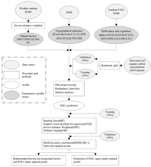
Figure 3.
Flow chart of the comparative assessment of algorithms.
As one of the standard spatial interpolation procedures, the IDW is a non-computationally and straightforward intensive method, which has been achieved in many geographic information system (GIS) software packages [38,39]. IDW is a deterministic method that assumes that the local impact of each point decreases with distance. Therefore, points closer to the location estimation are assigned a higher weight [38]. The IDW algorithm in this study was implemented in ArcGIS (version 10.2, Environmental Systems Research Institute, Redlands, CA, USA).
OK is a geostatistical technique and is widely used. Based on regionalized variables, it can generate an optimal unbiased estimated surface based on a semivariogram [15]. This semivariogram can be constructed with GS+ (version 9.0, Leland Stanford Junior University, Stanford, CA, USA). The RF algorithm is an integrated machine learning algorithm that uses combined multiple decision trees for supervised classification. The algorithm generates the final results by averaging the class allocation probabilities of all produced trees [40]. The trees are created by replacing (a bagging approach, also known as bootstrap aggregation) a subset of training samples and randomly selecting variables in RStudio software (version 1.1.456, Boston, MA, USA). The RF algorithm has advantages in classifying high-dimensional and confusing objects compared to other machine learning algorithms. It can also estimate the importance of predictor variables [41].
SVM is a non-linear machine learning method that derives an algorithm hyperplane. It describes the empirical data as accurately as possible and minimizes the distance from the hyperplane to the training data [42,43]. In this study, SVM was conducted using MATLAB software (version 2017a, Math Works, Natick, MA, USA). The validation set (n = 48) was used to test and compare the performance of the RF, SVM, IDW, and OK algorithms based on the root mean squared error (RMSE, Equation (1)), mean error (ME, Equation (2)), and correlation coefficient (r) between the measured and predicted values. The calculation equations for ME and RMSE are as follows [44], respectively:
where n is 48, is the predicted value of the SOCc (g·kg−1), is the measured value of the SOCc (g·kg−1), and ME is a measure of the predictive lack of bias. The closer the result is to 0, the more unbiased the method. The RMSE is a measure of prediction accuracy. The smaller the value, the more accurate the method.
3. Results
3.1. Descriptive Statistics of Wetland SOCc
The descriptive statistical values of wetland SOCc are listed in Table 2. The SOCc decreases with increasing depth and varies significantly between the three intervals (p < 0.05), with a mean SOCc value of 15.28 g·kg−1 for 0–30 cm, 7.57 g·kg−1 for 30–60 cm, and 5.22 g·kg−1 for 60–100 cm. The ranges of SOCc from the surface depth to the deep depth were 0.10 to 79.12, 0.03 to 68.25, and 0.02 to 67.41 g·kg−1, respectively. The variability of wetland SOCc in the study area can be expressed by the coefficient of variation (CV). CV values increased with soil intervals of 0–30, 30–60, and 60–100 cm.
Table 2.
Summary statistics for soil organic carbon concentration (SOCc).
3.2. Comparison of Different Algorithms
Table 3 presents the accuracies of different algorithms for predicting wetland SOCc. At 0–30 cm, the SVM algorithm yielded a mean error of −0.49 g·kg−1 and had the highest error. IDW had the lowest mean error at −0.03 g·kg−1, whereas RF performed best in predicting SOCc in terms of RMSE and r. At a depth of 30–60 cm, RF had the lowest RMSE and ME, as well as the largest r. At 60–100 cm, OK had the smallest ME. RF performed best in predicting the SOCc based on a larger RMSE and r than the other three algorithms. Therefore, considering the performance of the different algorithms at different depths, the RF is the best approach for spatially interpolating SOCc.
Table 3.
Accuracy assessment of the four algorithms. IDW: inverse distance weighted; OK: ordinary kriging; RF: random forest; SVM: support vector machine.
3.3. Effects of Environmental Variables on SOCc
Figure 4 documents the roles of the top five environmental variables in predicting SOCc using the RF algorithm. At a 0–30 cm depth, LST had the largest impact on the wetland SOCc, followed by NDVI, MAP, MAT, and H. At 30–60 cm, the LSWI and LST, characterizing the land surface’s hydrothermal conditions, exhibited notable influences on SOCc, whereas the MAT and MAP obtained from land meteorological observations had secondary influences. At 60–100 cm, the topographical factor H played a dominant role in affecting SOCc, followed by LST. Climatic factors, including MAT and MAP, were important factors influencing wetland SOCc. In general, LST, a remote sensing factor, performed the most important role in predicting the wetland SOCc in each examined soil depth.
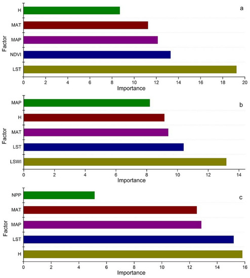
Figure 4.
Roles of the top five environmental variables in predicting wetland soil organic carbon concentration (SOCc) in different soil depths: (a) 0–30, (b) 30–60, and (c) 60–100 cm.
3.4. Spatial Patterns of Wetland SOCc in the Western Songnen Plain
The spatial patterns of wetland SOCc at different soil depths over the Western Songnen Plain estimated by the RF algorithm are shown in Figure 5. The wetlands in the northern study area were relatively concentrated, whereas wetlands in the south were relatively scattered. Larger wetland SOCc values were identified in the northern study area, and smaller values were identified in the south. The wetland SOCc at a 0–30 cm depth was significantly higher than that at 30–60 and 60–100 cm depths. With increasing soil depth, the wetland SOCc decreases accordingly.
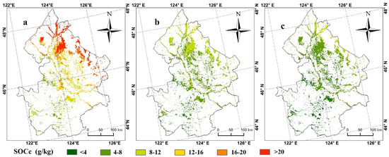
Figure 5.
Spatial patterns of wetland soil organic carbon concentration (SOCc) at different depths: (a) 0–30, (b) 30–60, and (c) 60–100 cm.
4. Discussion
4.1. Comparison of the Spatial Prediction Methods
In this study, RF performed better than the VR, IDW, and OK algorithms (Table 3). Although the IDW and OK spatial interpolation algorithms fully consider the spatial distance relationship, the accuracy of the RF algorithm is slightly higher than IDW and OK when considering the ME, RMSE, and r. Compared with SVM regression, the accuracy of the RF algorithm is much higher. Theoretically, OK and IDW consider the spatial autocorrelation of soil samples, whereas RF considers the spatial heterogeneity of environmental variables [45]. In other words, when the validation data are closer to the measured data in the soil sampling locations, the performance of OK and IDW is likely better than that of RF. Otherwise, when the spatial heterogeneity of environmental variables and their relationships with soil data are more significant, the performance of RF is likely superior. However, the spatial differences in wetlands SOCc are large and easily affected by environmental variables [5,6]. Therefore, interpolation based only on the autocorrelation of the sample data will result in slightly larger errors [45].
RF was used in previous studies for mapping soil organic content with climatic data, terrain data, remote sensing spectral data, and other auxiliary variables [14]. The processing of soil sample data and auxiliary variables was the same for the four algorithms. However, the RF algorithm was more accurate than the other three algorithms, as mentioned above.
4.2. Contolling Factors Affecting Spatial and Vertical Variations in Wetland SOCc
Environmental conditions affect the physicochemical properties of the soil to a certain extent [46]. Most wetlands accumulate water all year round. The duration for which the lands have been soaked by water also directly affects the growth and decomposition of wetlands’ organic carbon, thus affecting the SOCc [11]. For example, significant warming and drying trends have induced a soil organic carbon storage decline in croplands in the Sanjiang Plain [47]. Studies reported that the correlation between SOCc and environmental variables decreases with increasing soil depth [48]. Our study indicates that the relationship between SOCc and climatic factors gradually decreases with increasing soil depth. This means that topsoil organic carbon may be more sensitive to global climate change. Carbon stored in topsoil (e.g., 0–30 cm) will have been easily affected by warming temperature, which may further enhance the global greenhouse effect [49].
In the top soil layer, 0–30 cm, LST and MAT have a significant impact on SOCc. This shows that temperature plays an important role in the SOCc patterns. Temperature affects the decomposition rate, source, and sink process, as well as the soil density and water content of organic matter in wetlands [50]. Higher temperatures accelerate organic carbon decomposition and result in a lower SOCc [11]. Vegetation residues are conducive to the formation of humus and the enrichment of organic carbon [12]. Therefore, NDVI, characterizing vegetation conditions, has an important influence on SOCc. Precipitation is an important source of water replenishment in wetlands. The soil moisture content in wetlands has an important impact on soil microbial respiration, soil organic matter transport and sedimentation, and vegetation rot [11]. Therefore, at 0–30 cm, MAP has an important impact on SOCc. The annual average temperature in the Western Songnen Plain generally increases from north to south and is negatively correlated with soil organic carbon storage. MAP generally shows a decreasing trend from north to south. Annual precipitation is positively correlated with SOCc. Therefore, at 0–30 cm soil depth, LST, MAT, NDVI, and MAP have the strongest correlation with SOCc. The effects of temperature and precipitation on SOCc are long-term and stable [50]. Therefore, at 30–60 and 60–100 cm, MAT, MAP, LST, and LWSI also insignificantly influence SOCc. As the depth increases, the altitude’s importance score increases as SOCc increases.
4.3. Spatial and Vertical Variations in SOCc
The SOCc in the Western Songnen Plain decreases with soil depth. We found that the vertical distribution of wetland SOCc in the Western Songnen Plain is concentrated in the surface layer (0–30 cm). The soil organic carbon of the surface layer accounts for more than 50% of the total depth of 1 m, which is similar to the estimation of global soil organic carbon [51].
A higher wetland SOCc was identified in the Western Songnen Plain than in China’s wetlands overall, which supports previous findings that the SOCc in northeast China is higher than in southern China [52,53], mostly due to the lower temperature in northeast compared to southern China and higher precipitation than that in western China [54]. Low temperatures and high precipitation are beneficial for stabilizing soil organic carbon storage. Also, as the latitude increases, the temperature decreases [55]. Therefore, in the western part of the Songnen Plain, the closer the area is to the north, the higher the wetland SOCc.
For different soil depths, the SOCc values at 0–30 cm have the largest difference from the other groups, whereas those at 60–100 cm have the smallest. In the 0–30 cm soil layer, the SOCc near the northern part of the study area was estimated to be higher than 20 g·kg−1, whereas the SOCc in the southern part is lower than 4 g·kg−1. Surface soil is affected more by the environment. Thus, small changes in the environment can affect the storage and release of surface soil organic carbon. The north–south differences in environmental factors, such as temperature and precipitation, cause huge variations in SOCc in the top soil layer. As soil depth increases, the SOCc is less affected by the environment. Therefore, the spatial heterogeneity of SOCc at 60–100 cm is significantly reduced compared to that at 0–30 cm.
5. Conclusions
The observed changes in SOCc were estimated using different methods of remote sensing and geographic information systems. Our results showed that SOCc decreases with increasing soil depth, and that the coefficient of variation increased with increasing soil depth in the 160 wetland soil sample sites. The measured SOCc values at the depths of 0–30, 30–60, and 60–100 cm were 15.28, 7.57, and 5.22 g·kg−1, respectively. Among the different methods, RF was the most accurate. The influence of different factors on SOCc showed that surface soil is more affected by environmental variables. MAT, MAP, LST, and LWSI also influence SOCc. The distribution of wetlands in the northern part of the study area is relatively concentrated, and the SOCc value in the north is also significantly higher than in the south.
Author Contributions
Y.R., X.L., Z.W., D.M., M.J., and L.C. conceived and designed the experiments; Y.R. and L.C. performed the experiments; Y.R. and L.C. analyzed the data; Y.R., X.L., Z.W., and D.M. contributed reagents, materials, and analysis tools. Y.R., X.L., and L.C. wrote the paper, and Z.W. and D.M. revised the manuscript. All authors have read and agreed to the published version of the manuscript.
Funding
This research was funded by the National Natural Science Foundation of China (No. 41671219, 41730643, and 41771383), the Outstanding Young Scientist Foundation of Institute of Northeast Geography and Agroecology (IGA), Chinese Academy of Sciences (No. Y5H1061001), and the funding from Youth Innovation Promotion Association of CAS (2017277, 2012178).
Acknowledgments
We are very grateful to those who participated in the field soil surveys and thank the National Earth System Science Data Center of China for supporting geographic data (http://www.geodata.cn).
Conflicts of Interest
The authors declare no conflict of interest.
References
- Hadi, A.; Inubushi, K.; Furukawa, Y.; Purnomo, E.; Rasmadi, M.; Tsuruta, H. Greenhouse gas emissions from tropical peatlands of Kalimantan, Indonesia. Nutr. Cycl. Agroecos. 2005, 71, 73–80. [Google Scholar] [CrossRef]
- Bernal, B.; Mitsch, W.J. A comparison of soil carbon pools and profiles in wetlands in Costa Rica and Ohio. Ecol. Eng. 2008, 34, 311–323. [Google Scholar] [CrossRef]
- Mitra, S.; Wassmann, R.; Vlek, P.L.G. An appraisal of global wetland area and its organic carbon stock. Curr. Sci. 2005, 88, 25–35. [Google Scholar]
- Stockmann, U.; Adams, M.A.; Crawford, J.W.; Field, D.J. The knowns, known unknowns and unknowns of sequestration of soil organic organic carbon. Agric. Ecosyst. Environ. 2013, 164, 80–99. [Google Scholar] [CrossRef]
- Cambardella, C.; Moorman, T.; Parkin, T.; Karlen, D.; Novak, J.; Turco, R.; Konopka, A. Field-scale variability of soil properties in central Iowa soils. Soil Sci. Soc. Am. J. 1994, 58, 1501–1511. [Google Scholar] [CrossRef]
- Liu, D.; Wang, Z.; Zhang, B.; Song, K.; Li, X.; Li, J.; Li, F.; Duan, H. Spatial distribution of soil organic carbon and analysis of related factors in croplands of the black soil region, Northeast China. Agric. Ecosyst. Environ. 2006, 113, 73–81. [Google Scholar] [CrossRef]
- Zhang, S.; Zhang, X.; Huffman, T.; Liu, X.; Yang, J. Influence of topography and land management on soil nutrients variability in Northeast China. Nutr. Cycl. Agroecosyst. 2011, 89, 427–438. [Google Scholar] [CrossRef]
- Bhandari, K.B.; West, C.P.; Acosta-Martinez, V. Assessing the role of interseeding alfalfa into grass on improving pasture soil health in semi-arid Texas High Plains. Appl. Soil Ecol. 2020, 147, 103399. [Google Scholar] [CrossRef]
- Bhandari, K.B.; West, C.P.; Longing, S.D.; Brown, C.P.; Green, P.E. Comparison of Arthropod Communities among Different Forage Types on the Texas High Plains using Pitfall Traps. Crop Forage Turfgrass Manag. 2018, 4, 180005. [Google Scholar] [CrossRef]
- Bhandari, K.B.; West, C.P.; Klein, D.; Subbiah, S.; Surowiec, K. Essential oil composition of ‘WW-B.Dahl’ old world bluestem (Bothriochloa bladhii) grown in the Texas High Plains. Ind. Crop Prod. 2019, 133, 1–9. [Google Scholar] [CrossRef]
- Zhi, P.L.; Ming, A.S.; Yun, Q.W. Effect of environmental factors on regional soil organic carbon stocks across the Loess Plateau region, China. Agric. Ecosyst. Environ. 2011, 142, 184–194. [Google Scholar]
- Ganuza, A.; Almendros, G. Organic carbon storage in soils of the Basque Country (Spain): The effect of climate, vegetation type and edaphic variables. Biol. Fertil. Soils 2003, 37, 154–162. [Google Scholar] [CrossRef]
- Dai, W.; Huang, Y. Relation of soil organic matter concentration to climate and altitude in zonal soils of China. Catena 2005, 65, 87–94. [Google Scholar] [CrossRef]
- Kennedy, W.; Dieu, T.B.; Øystein, B.D. A comparative assessment of support vector regression, artificial neural networks, and random forests for predicting and mapping soil organic carbon stocks across an Afromontane landscape. Ecol. Indic. 2015, 52, 394–403. [Google Scholar]
- Chen, L.; Ren, C.Y.; Li, L. A Comparative Assessment of Geostatistical, Machine Learning, and Hybrid Approaches for Mapping Topsoil Organic Carbon Content. ISPRS Int. J. Geo-Inf. 2019, 8, 174. [Google Scholar] [CrossRef]
- Veeraswamy, G.; Nagaraju, A.; Balaji, E.; Sreedhar, Y.; Narasimhlu, K.; Harish, P. Data sets on spatial analysis of hydro geochemistry of Gudur area, SPSR Nellore district by using inverse distance weighted method in Arc GIS 10.1. Data Brief 2019, 22, 1003–1010. [Google Scholar]
- Lian, G.; Guo, X.D.; Fu, B.J.; Hu, C.X. Prediction of the spatial distribution of soil properties based on environmental correlation and geostatistics. Trans. Chin. Soc. Agric. Eng. 2009, 25, 112–122. [Google Scholar]
- Malone, B.P.; McBratney, A.B.; Minasny, B.; Laslett, G.M. Mapping continuous depth functions of soil carbon storage and available water capacity. Geoderma 2009, 154, 138–152. [Google Scholar] [CrossRef]
- Jaber, S.M.; Al-Qinna, M.I. Soil organic carbon modelling and mapping in a semi-arid environment using thematic mapper data. Photogramm. Eng. Remote Sens. 2011, 77, 709–719. [Google Scholar] [CrossRef]
- Li, Q.; Yue, T.; Wang, C.; Zhang, W.; Yu, Y.; Li, B.; Yang, J.; Bai, G. Spatially distributed modeling of soil organic matter across China: An application of artificial neural network approach. Catena 2013, 104, 210–218. [Google Scholar] [CrossRef]
- Rossel, R.A.V.; Behrens, T. Using data mining to model and interpret soil diffuse reflectance spectra. Geoderma 2010, 158, 46–54. [Google Scholar] [CrossRef]
- Khlosi, M.; Alhamdoosh, M.; Doualk, A.; Gabriels, D.; Cornelis, W.M. Enhanced pedotransfer functions with support vector machines to predict water retention of calcareous soil. Eur. J. Soil Sci. 2016, 67, 276–284. [Google Scholar] [CrossRef]
- Martin, M.P.; Wattenbach, M.; Smith, P.; Meersmans, J.; Jolivet, C.; Boulonne, L.; Arrouays, D. Spatial distribution of soil organic carbon stocks in France. Biogeosciences 2011, 8, 1053–1065. [Google Scholar] [CrossRef]
- Grimm, R.; Behrens, T.; Märker, M.; Elsenbeer, H. Soil organic carbon concen- trations and stocks on Barro Colorado Island-Digital soil mapping using Random Forests analysis. Geoderma 2008, 146, 102–113. [Google Scholar] [CrossRef]
- Wiesmeier, M.; Barthold, F.; Blank, B.; Kögel-Knabner, I. Digital mapping of soil organic matter stocks using Random Forest modeling in a semi-arid steppe ecosystem. Plant Soil 2011, 340, 7–24. [Google Scholar] [CrossRef]
- Vågen, T.G.; Winowiecki, L.A.; Abegaz, A.; Hagdu, K.M. Landsat-based approaches for mapping of land degradation prevalence and soil functional properties in Ethiopia. Remote Sens. Environ. 2013, 134, 266–275. [Google Scholar] [CrossRef]
- Drake, J.M.; Randin, C.; Guisan, A. Modelling ecological niches with support vector machines. J. Appl. Ecol. 2006, 43, 424–432. [Google Scholar] [CrossRef]
- Wang, Z.M.; Huang, N.; Luo, L. Shrinkage and fragmentation of marshes in the West Songnen Plain, China, from 1954 to 2008 and its possible causes. Int. J. Appl. Earth Obs. Geoinf. 2011, 13, 477–486. [Google Scholar] [CrossRef]
- Wang, Z.M.; Song, K.S.; Zhang, B.; Liu, D.W.; Ren, C.Y.; Luo, L.; Yang, T.; Huang, N.; Hu, L.J.; Yang, H.J.; et al. Shrinkage and fragmentation of grasslands in the West Songnen Plain, China. Agric. Ecosyst. Environ. 2009, 129, 315–324. [Google Scholar] [CrossRef]
- Mao, D.H.; Luo, L.; Wang, Z.M.; Wilson, M.C.; Zeng, Y.; Wu, B.F.; Wu, J.G. Conversions between natural wetlands and farmland in China: A multiscale geospatial analysis. Sci. Total Environ. 2018, 634, 550–560. [Google Scholar] [CrossRef]
- Mao, D.H.; He, X.Y.; Wang, Z.M.; Tian, Y.L.; Xiang, H.X.; Yu, H.; Man, W.; Jia, M.M.; Ren, C.Y.; Zheng, H.F. Diverse policies leading to contrasting impacts on land cover and ecosystem services in Northeast China. J. Clean. Prod. 2019, 240, 117961. [Google Scholar] [CrossRef]
- Hardisky, M.A.; Gross, M.F.; Klemas, V. Remote-Sensing of Coastal Wetlands. BioScience 1986, 36, 453–460. [Google Scholar] [CrossRef]
- Mao, D.H.; Wang, Z.M.; Li, L.; Miao, Z.H.; Ma, W.H.; Song, C.C.; Ren, C.Y.; Jia, M.M. Soil organic carbon in the Sanjiang Plain of China: Storage, distribution and controlling factors. Biogeosciences 2015, 12, 1635–1645. [Google Scholar] [CrossRef]
- Li, J.W.; Richter, D.D.; Mendoza, A.; Heine, P. Effects of land-use history on soil spatial heterogeneity of macro- and trace elements in the Southern Piedmont USA. Geoderma 2010, 156, 60–73. [Google Scholar] [CrossRef]
- Mao, D.H.; Wang, Z.M.; Wu, J.G.; Wu, B.F.; Zeng, Y.; Song, K.S.; Yi, K.P.; Luo, L. China’s wetlands loss to urban expansion. Land Degrad. Dev. 2018, 29, 2644–2657. [Google Scholar] [CrossRef]
- Whigham, D.F.; Simpson, R.L. The relationship between aboveground and belowground biomass of freshwater tidal wetland macrophytes. Aquat. Bot. 1978, 5, 355–364. [Google Scholar] [CrossRef]
- Sjörs, H. Peat on Earth: Multiple Use or Conservation? Ambio 1980, 9, 303–308. [Google Scholar]
- Tang, G.A.; Yang, X. ArcGIS Experimental Course for Spatial Analysis; Science Press: Beijing, China, 2013. [Google Scholar]
- Lu, G.Y.; Wong, D.W. An adaptive inverse-distance weighting spatial interpolation technique. Comput. Geosci. 2008, 34, 1044–1055. [Google Scholar] [CrossRef]
- Liu, Y.L.; Guo, L.; Jiang, Q.H.; Zhang, H.T.; Chen, Y.Y. Comparing geospatial techniques to predict SOC stocks. Soil Till. Res. 2015, 148, 46–58. [Google Scholar] [CrossRef]
- Akpa, S.I.C.; Odeh, I.O.A.; Bishop, T.F.A.; Hartemink, A.E.; Amapu, I.Y. Total soil organic carbon and carbon sequestration potential in Nigeria. Geoderma 2016, 271, 202–215. [Google Scholar] [CrossRef]
- Keskin, H.; Grunwald, S.; Harris, W.G. Digital mapping of soil carbon fractions with machine learning. Geoderma 2019, 339, 40–58. [Google Scholar] [CrossRef]
- Vapnik, V.N. The Nature of Statistical Learning Theory; Springer: New York, NY, USA, 2000. [Google Scholar]
- Platt, J. Fast Training of Support Vector Machines Using Sequential Minimal Optimization; MIT Press: Cambridge, MA, USA, 1999. [Google Scholar]
- Song, Y.Q.; Yang, L.A.; Li, B.; Hu, Y.M.; Wang, A.L.; Zhou, W.; Cui, X.S.; Liu, Y.L. Spatial prediction of soil organic matter using a hybrid geostatistical model of an extreme learning machine and ordinary kriging. Sustainability 2017, 9, 754. [Google Scholar] [CrossRef]
- Odum, W.E.; Odum, E.P.; Odum, H.T. Nature’s pulsing paradigm. Estuaries 1995, 8, 547. [Google Scholar] [CrossRef]
- Man, W.D.; Yu, H.; Li, L. Spatial Expansion and Soil Organic Carbon Storage Changes of Croplands in the Sanjiang Plain, China. Sustainability 2017, 9, 563. [Google Scholar] [CrossRef]
- Bhandari, K.B.; West, C.P.; Acosta-Martinez, V.; Cotton, J.; Cano, A. Soil health indicators as affected by diverse forage species and mixtures in semi-arid pastures. Appl. Soil Ecol. 2018, 132, 179–186. [Google Scholar] [CrossRef]
- Lees, K.J.; Quaife, T.; Artz, R.R.E.; Khomik, M.; Clark, J.M. Potential for using remote sensing to estimate carbon fluxes across northern peatlands—A review. Sci. Total Environ. 2018, 618, 857–874. [Google Scholar] [CrossRef]
- Eric, A.D.; Ivan, A.J. Temperature sensitivity of soil carbon decomposition and feedbacks to climate change. Nature 2006, 440, 165–173. [Google Scholar]
- Eswaran, H.; Berg, E.V.D.; Reich, P. Organic Carbon in Soils of the World. Soil Sci. Soc. Am. J. 1993, 57, 192–194. [Google Scholar] [CrossRef]
- Song, G.H.; Li, L.Q.; Pan, G.X.; Zhang, Q. Topsoil organic carbon storage of China and its loss by cultivation. Biogeochemistry 2005, 74, 47–62. [Google Scholar] [CrossRef]
- Huang, Y.; Sun, W.J. Changes in topsoil organic carbon of croplands in mainland China over the last two decades. Chin. Sci. Bull. 2006, 51, 1785–1803. [Google Scholar] [CrossRef]
- Pan, G.X.; Li, L.Q.; Wu, L.S.; Zhang, X.H. Storage and sequestration potential of topsoil organic carbon in China’s paddy soils. Glob. Chang. Biol. 2004, 10, 79–92. [Google Scholar] [CrossRef]
- Post, W.M.; Emanuel, W.R.; Zinke, P.J.; Stangenberger, A.G. Soil carbon pools and world life zones. Nature 1982, 298, 156–159. [Google Scholar] [CrossRef]


© 2020 by the authors. Licensee MDPI, Basel, Switzerland. This article is an open access article distributed under the terms and conditions of the Creative Commons Attribution (CC BY) license (http://creativecommons.org/licenses/by/4.0/).