Article

Development of an Optimal Model for the Xiluodu-Xiangjiaba Cascade Reservoir System Considering the Downstream Environmental Flow

1
College of Hydraulic and Environmental Engineering, China Three Gorges University, Yichang 443002, China
2
China Three Gorges Corporation, Beijing 100038, China
3
China Yangtze Power Corporation, Yichang 443002, China
4
Helmholtz Centre for Environmental Research, Brueckstr 3a, D-39114 Magdeburg Germany
*
Author to whom correspondence should be addressed.
Sustainability 2020, 12(3), 966; https://doi.org/10.3390/su12030966
Submission received: 11 December 2019 / Revised: 25 January 2020 / Accepted: 26 January 2020 / Published: 29 January 2020
(This article belongs to the Section Environmental Sustainability and Applications)

Abstract

:
To explore the influence of the Xiluodu-Xiangjiaba cascade reservoir system on the appropriate environmental flow (AEF) of the Jinsha River, a multiobjective optimal cascade reservoir model was established with the aim of maximizing power generation while minimizing the downstream degree of AEF alteration. The AEF was determined using the range of variability approach (RVA). The optimal model was solved using an improved version of NSGA-II called INSGA2-DS. Inflows in typical normal and dry years were selected for optimization. The results show that in a normal year, power generation can be increased by 1.28% compared with that under the current regular operation conditions by prioritizing the maximization of power generation, in which case the degree of AEF alteration will increase by 13.86%. In contrast, the degree of AEF alteration will decrease by 22.53% if ecological protection is prioritized, but power generation will decrease by 0.62%. Similarly, in a dry year, power generation can be increased by 1.76% compared with that under the current regular operation conditions to maximize economic benefit, in which case, the degree of AEF alteration will increase by 4.95%. By contrast, the degree of AEF alteration can be decreased by 13.70% if the objective is AEF minimization, but power generation will decrease by 0.48%. These research results provide useful information for the formulation of ecological operation schemes involving cascade reservoirs on the Jinsha River.

1. Introduction

Among all renewable energy sources, hydropower is the most commonly used for electricity production, with the corresponding global capacity having increased by more than 30% between 2007 and 2015 [1,2]. In the past three decades, reservoirs and hydropower stations have been rapidly developed to provide clean energy and reduce greenhouse gas emissions in China [3,4]. One of the most prevalent ways to take full advantage of available hydropower resources is to build cascade reservoirs along a river [5,6]. Relative to the total revenue generated by the operation of independent reservoirs, synergistic benefits can be achieved through the coordinated operation of cascade reservoirs [7]. Generally, the main objective of cascade reservoirs is to maximize energy and revenue yields [8,9]. However, this strategy has an adverse impact on downstream river ecosystems. In addition to providing economic benefits, reservoirs also serve other purposes, including providing sufficient water for downstream habitats to maintain aquatic biodiversity, irrigation for agriculture, recreational opportunities, and domestic and industrial water supplies [10,11].
The Xiluodu-Xiangjiaba cascade reservoir system is located in the lower reaches of the Jinsha River [12]. The lower reaches of the Jinsha River are also a pivotal part of the “National Nature Conservation Zone of Rare Fishes” [13,14]. With its exceptional flow pattern, climate and natural environment, the conservation zone is home to abundant and diverse communities of aquatic organisms, among which fish resources are particularly abundant. The zone includes more than 70 types of rare and endemic fishes, such as Coreius guichenoti, Acipenser dabryanus, and the Chinese sucker fish [15,16]. After the cascade reservoir system started operation, the downstream flow changed greatly, especially during the impoundment period in September. These changes directly affected the habitats of rare fish species in the lower reaches at various spatial and temporal scales. The number of fish species and the average size of the fish have decreased, and juvenile populations have also been decreasing [17,18].
Flow is the main driving force affecting the physical habitat conditions of a river, which, in turn, are the main factors determining biological composition [19,20]. The water allocated for a river ecosystem must be within the range of the natural variability of the flow regime. In the absence of environmental constraints, the pursuit of economic benefits may lead to dramatic changes in the environmental flow regime, which will have a negative impact on human settlements, aquatic biodiversity, agriculture and recreational activities [21,22]. Thus, there is an urgent need to take effective measures to alleviate this problem.
Many studies have shown that the appropriate environmental flow (AEF) for downstream areas can be maintained through reservoir optimization [23,24]. Zhang et al., established a multiobjective optimization model with the aim of maximizing the annual power generation while minimizing the degree of ecological change in the lower reaches of the Lancang River [25]; Takada et al. developed a method for constructing optimal operation curves considering environmental water supplies for the Dau Tieng Reservoir [26]; Sichilalu et al. presented an optimal control model for a wind-hydrokinetic powered pumpback operation of a hydropower plant with stringent regulatory requirements on downstream environmental flows [27]; Stuart et al. developed the building block method of environmental flows to enhance the abundance of juvenile Murray cod and promote population recovery [28]. Notably, several researchers have previously studied the optimization of the Xiluodu-Xiangjiaba cascade reservoir system. However, most of these researchers have focused on only a single objective, such as electricity production, impoundment, navigation, or sediment loading, and the flow has been considered only as a constraint condition [29]. In contrast to these previous approaches, efforts to achieve the ecological optimization of reservoirs must consider both economic and ecological objectives; nevertheless, these two types of objectives may conflict, with efforts to pursue the optimum for one objective inevitably reducing performance in terms of another objective [30,31]. To minimize the negative impact of cascade reservoir operations, a regulatory policy for the downstream environmental flow must be incorporated into the optimal policy, which typically reduces operational flexibility and therefore reduces revenue-generating capacity [32,33].
In the present study, the downstream AEF is considered as an objective function. Based on the river discharge, the AEF is determined using the range of variability approach (RVA). Then, an ecologically oriented optimization model was established to obtain an optimal curve that balances the economic and ecological requirements of the cascade reservoir system during impoundment. Finally, the model was optimized using an improved nondominated sorting genetic algorithm based on dominance strength (INSGA2-DS). The results of this study could provide useful information to help water conservancy institutions and policy makers improve the sustainable management of cascade reservoirs in the lower reaches of the Jinsha River.

2. Materials and Methods

2.1. Study Area

The lower reaches of the Jinsha River (from Panzhihua to Yibin) represent some of the most abundant river resources in China. Four cascade reservoirs, namely, the Wudongde (WDD), Baihetan (BHT), Xiluodu (XLD) and Xiangjiaba (XJB) Reservoirs, either are under construction or have been completed. (Figure 1). Xiluodu and Xiangjiaba were first-phase projects, for which impoundment began in 2013 and 2012, respectively. The installed capacities of these two hydropower stations are 12,600 MW and 6000 MW, respectively [34,35]. The hydraulic connection between the two reservoirs is tight, forming a cascade reservoir system with effective joint operation conditions, the main parameters of these two reservoirs are listed in Table 1.

2.2. Model Establishment

2.2.1. Objective Functions

The objectives of the model were to maximize total hydropower generation and to minimize the degree of AEF alteration. These two objectives are mutually conflicting because maximizing hydropower production requires increasing the water level in the reservoir, while minimizing the degree of AEF alteration requires more water to be released from the reservoir for downstream needs [36] These two competing objectives of the system are expressed as follows.
(1) Maximizing the hydropower generation of the overall system
f 1 = max t = 1 T ( P t X L D + P t X J B ) · Δ t
(2) Minimizing the degree of AEF alteration
f 2 = min 1 T t = 1 T ( | Q t X J B , o u t Q A E F , t | ) / Q A E F , t
where T is the total optimization period; t is the time step index; P t X L D and P t X J B are the outputs of the Xiluodu and Xiangjiaba hydropower stations, respectively, in the t th time step; Δ t is the length of a time step; Q t X J B , o u t is the release from the Xiangjiaba Reservoir in the t th time step; and Q A E F , t is the downstream AEF. The detailed solution process is described in Section 3.2.

2.2.2. Constraint Conditions

The operation constraints of a reservoir include constraints on the water level, water balance, output and outflow. The specific constraints considered in this study are as follows.
(1) Restriction on the reservoir water level:
Z t i , min Z t i Z t i , max
where Z t i , Z t i , min , and Z t i , max are the actual, minimum, and maximum water levels, respectively, of reservoir i in time step t .
(2) Water balance constraint:
V t + 1 i = V t i + ( I t i Q T t i Q S t i ) · Δ t
where V t + 1 i and V t i are the capacities of reservoir i at the beginning of time steps t and t + 1 , respectively; I t i is the inflow to reservoir i ; Q T t i is the outflow from the turbines; and Q S t i is the spillway or outlet flow that cannot be utilized for power generation. Together, Q T t i and Q S t i reflect the total outflow from the reservoir.
(3) Spatial transition flow constraint:
I t i + 1 = I P t i + 1 + Q T t i + Q S t i
where I P t i + 1 denotes the inflow between power stations i and i + 1 generated by precipitation. This equation indicates that the total inflow to reservoir i + 1 consists of the inflow generated between reservoirs i and i + 1 , and the total outflow from reservoir i .
(4) Output constraint:
P t i , min P t i P t i , max
where P t i , min and P t i , max are the minimum and maximum outputs, respectively, of reservoir i .
(5) Outflow constraint
Q t i , min Q t i Q t i , max
where Q t i , min and Q t i , max are the minimum and maximum permitted outflows, respectively, of reservoir i .
(6) Nonnegativity constraint:
V t i ,   Q t i , P t i 0

2.2.3. Penalty Functions

It is difficult to satisfy all constraints simultaneously. To this end, two methods can be used to address all constraints during the process of optimization [37]. The first method involves setting certain limits, such as reservoir water level limits, when generating the initial population and developing a new generation. The second method is to determine whether a condition is satisfied after performing the necessary calculations and then to remove infeasible solutions by means of a penalty function [38,39]. Such a penalty function penalizes individuals based on violations of constraints. In this study, the penalty function approach was used to reduce the applicability of infeasible solutions in order to encourage the selection of feasible solutions. Initially, the extent of constraint violation is calculated as follows:
c 1 = max ( C min C , 0 ) c 2 = max ( C C max , 0 )
where c 1 and c 2 represent the constraint violations, C is a constraint, and C min and C max represent the allowable constraint scope of each solution. Thus, c can be expressed as follows:
c = ( c 1 + c 2 ) / 2
where c represents the average extent of violation of constraint C . Then, the corresponding penalty value is calculated as follows:
P = 1 + β
β = j = 1 N C i = 1 N X c j i ,   i = 1 , 2 , , N X ;   j = 1 , 2 , , N C
c j i = { 0 c j i    x f e a s i b l e x f e a s i b l e
where P is the penalty value, β is the penalty parameter, N X is the number of genes, N C is the number of constraints, and c j i is the penalty function for the j th constraint on the i th variable.
When the objective is to determine the minimum value, the objective function value is multiplied by the penalty value:
F m = f m P
When the objective is to determine the maximum value, the objective function value is divide by the penalty value.
F m = f m / P
In Equations (13) and (14), F m is the penalized objective function, and f m is the objective function.
Constraints can be divided into three categories: boundary constraints, soft constraints, and hard constraints. Boundary constraints (Equation (3)) limit the search space for the design task. Soft constraints (Equations (6) and (7)) are enforced by means of penalties, which will slightly reduce the applicability of solutions with low levels of violation and significantly reduce the applicability of solutions with high levels of violation; consequently, such constraints are not strictly related to certain levels of violation. The degree of violation of soft constraints will guide the optimization algorithm towards the feasible solution space during the search process. The constant coefficient of a penalty term cannot be set to too large a value because doing so would make an optimal fitness value difficult to obtain.
During the calculation process, if various genes have reached their limiting conditions, then corresponding penalties must be imposed in accordance with the degrees of violation of these limits. Consequently, the fitness value will change rapidly. The penalty functions for the various limiting conditions are defined as described below.
When Q t , i < 0 , the corresponding solution is impossible, and the penalty function associated with the violation of this physical condition involves multiplying the obtained negative release value by the appropriate penalty value:
c 1 t X L D = 1000 . Q t X L D , o u t . c 1 X L D c 1 t X J B = 1000 . Q t X J B , o u t c 1 X J B
where c 1 t represents the average extent of violation of the release constraint.
For flood control of the Jinsha River, a penalty function is established based on the requirement that Q t X J B , o u t > Q t X J B , o u t , max . This penalty function is formulated as follows:
c 2 t X J B = ( Q t X J B , o u t , max Q t X J B , o u t ) . c 2 t
where c 2 t represents the average extent of violation of the release constraint.
For power generation, we establish penalty functions based on the requirements that Q t g < Q t g , min and P t < P t min . These penalty functions are formulated as follows:
c 3 t X L D = ( Q t X L D , g Q t X L D , g , min ) . c 3 t X L D c 4 t X L D = ( N t X L D N t X L D , min ) . c 4 t X L D
c 3 t X J B = ( Q t X J B , g Q g X J B , g , min ) . c 3 t X J B c 4 t X J B = ( N t X J B N t X J B , min ) . c 4 t X J B
where c 3 t X L D and c 4 t X L D represent the average levels of violation of the turbine release and reservoir outflow constraints ( Q t X L D , g > Q t X L D , g , max ), respectively, for the Xiluodu Reservoir and c 3 t X J B and c 4 t X J B represent the average levels of violation of the turbine release and reservoir release constraints ( Q t X J B , g > Q t X J B , g , max ), respectively, for the Xiangjiaba Reservoir.
To maintain the ecological base flow demand in the downstream area, if the reservoir release is less than the ecological base flow demand, we apply the following penalty function:
c 5 t X J B = ( Q t X J B , o u t Q t X J B , o u t , min ) . c 5 t
where c 5 t represents the average extent of violation of the release constraint associated with the minimum downstream environmental flow. The penalty parameter β is the sum of all levels of constraint violation:
β = t = 1 N X ( c 1 t X L D + c 1 t X J B + c 2 t X J B + c 3 t X L D + c 3 t X J B + c 4 t X L D + c 4 t X J B + c 5 t X J B )
The coefficients defined in the above functions are mainly subjective, and several trial-and-error processes must be conducted to effectively obtain suitable solutions.

2.3. Model Solution

The goal of a single-objective optimization problem is to obtain an optimal solution by searching for the minimum or maximum value of the objective function. However, in real life, most water resource optimization problems involve conflicting objectives, for which there is no efficient method of finding optimal solutions with multiple trade-offs. The goal of such a multiobjective problem is to find an optimal solution for all targets, also known as a Pareto-optimal solution.
The nondominated sorting genetic algorithm II (NSGA-II) is a fast elite multiobjective algorithm that follows the NSGA framework [40,41,42]. This method has been effectively implemented to address various water management issues. However, this algorithm has many deficiencies when solving for the Pareto boundaries of high-dimensional multivariable and complex nonlinear multiobjective problems, such as an inability to identify pseudo-nondominated solutions, an unreasonable crowding distance formula, and high computational complexity.
This paper uses an improved algorithm based on NSGA-II, namely, INSGA2-DS. The pseudodominated solutions in the nondominated solution set are selected by introducing the concept of a dominance intensity order, and a new crowding distance formula that considers the variance is adopted. For calculating the crowding distance, an adaptive elite retention strategy is introduced to control the scale of elite retention, and other means are also adopted to speed up the calculation efficiency. The details of the improved algorithm are introduced as follows.

2.3.1. Fast Nondominated Sorting

NSGA-II uses the fast nondominated sorting method to determine the nondominated level and sort by comparing the dominance relations between each pair of individuals. However, this method results in a large number of pseudo-nondominated solutions in the nondominated set, which reduces the convergence efficiency and solution quality. To remove these pseudo-nondominated solutions, a measure called the dominance intensity is introduced as follows:
ξ i = k = 1 m ( f k ( i ) f k min f k max f k min )
where ξ i is the dominance intensity of the ith member of the population, m is the number of subobjectives, and f k max and f k min are the maximum and minimum values, respectively, of the kth subobjective in the nondominated set.

2.3.2. Distribution Retention Method

The concept of distribution here refers to the degrees of similarity and difference along the real Pareto boundary, reflecting the uniformity and diversity of the solution set. NSGA-II considers only the distances between neighboring individuals. However, individuals with different degrees of crowding distance with respect to different subobjectives cannot yield more genetic opportunities, and this situation is not conducive to maintaining the solution distribution. Therefore, a new crowding distance formula that considers the variance is introduced as follows:
{ i D = i d { 1 m j = 1 m [ ( | f j i + 1 f j i 1 | ) i d m ] 2 } 1 + 1 i d = j = 1 m ( | f j i + 1 f j i 1 | )
where i D is the crowding distance obtained with the new method, id is the crowding distance in NSGA-II, and f j i + 1 and f j i 1 are the values of the jth subobjective for individuals i+1 and i-1, respectively. After the above calculations, each individual member of the population is associated with three parameters: a nondominated set rank (rank), a dominance intensity (ξ) and a crowding distance ( i D ). The priorities of these parameters are ordered as follows: rank (smaller is better) > i D (larger is better) > ξ (smaller is better).

2.3.3. Adaptive Elite Retention Strategy

The elite retention scale of NSGA-II is a fixed value, which is not conducive to solution set convergence. In the improved algorithm, an adaptive elite retention strategy is adopted. In the early stage of evolution, the elite retention scale is set to increase the diversity of the solutions. In the later stage of evolution, the elite retention scale is set to improve the convergence of the algorithm. The number of elites in the population of the gth generation, E g , is calculated as follows:
E g = P × α g
where α g is the impact factor for the number of gth-generation elites and P is the population size. The value of α g is adaptively and iteratively calculated as follows:
α g + 1 = α g [ 1 + ln ( ρ + 1 ) ]
where α g + 1 is the impact factor for the number of (g+1)th-generation elites and ρ is the ratio of the number of solutions in the nondominated set in the gth-generation population to the total population size P.
The improved algorithm, INSGA2-DS, consists of five main operations: initialization, crossover and mutation, fast nondominated sorting, implementation of elite crowding comparison operators, and termination and output of results.
The loop structure of INSGA2-DS is shown in Figure 2. P t is the parent population, and P c and P m are the offspring populations. F 1 ,   F 2   , ,   F k are solution classes. F 1 is the best solution set among the parents and offspring, F 2 is the second-best solution set, etc.
The approach for using INSGA2-DS to solve the problem considered in this paper is illustrated in Figure 3.

2.3.4. Parameter Setting

For this study, the INSGA2-DS optimization model was programmed based on MATLAB. The population size was set to 30, the maximum number of iterations was 1500, the crossover probability was 0.75, the mutation probability was 0.01, and 30 Pareto-optimal schemes were obtained through the corresponding calculations.

3. Results and Discussion

3.1. Optimization Period and Typical Years

In accordance with the typical operation and regulation of cascade reservoirs, the Xiluodu Reservoir operates at a limiting water level of 560.0 m during the flood season (from June 1 to September 10); then, it begins to store water on September 10, and the water level reaches 600.0 m at the end of September. The Xiangjiaba Reservoir operates at 370.0 m during the flood season and then also starts to store water on September 10 and the water level reaches 380.0 m at the end of September. However, recent research has shown that the flood control capacity of cascade reservoirs may somewhat decrease from the end of August to early September. Therefore, to improve the reservoir storage fill rate and reduce the impact of water storage downstream, the impoundment time should be advanced to the end of August.
Considering both the downstream environmental flow requirements and the calculation time, we divided the data to be analyzed into subperiods. Reservoir managers often use cycles of 5 days when making operation plans during the impoundment period. In terms of calculation efficiency, either 5 or 6 days is a suitable time interval; therefore, the entire period of interest was divided into 8 subperiods, with the first subperiod being Aug. 21–25, the second subperiod being Aug. 26–31, the third subperiod being Sep. 1–5, and so on.
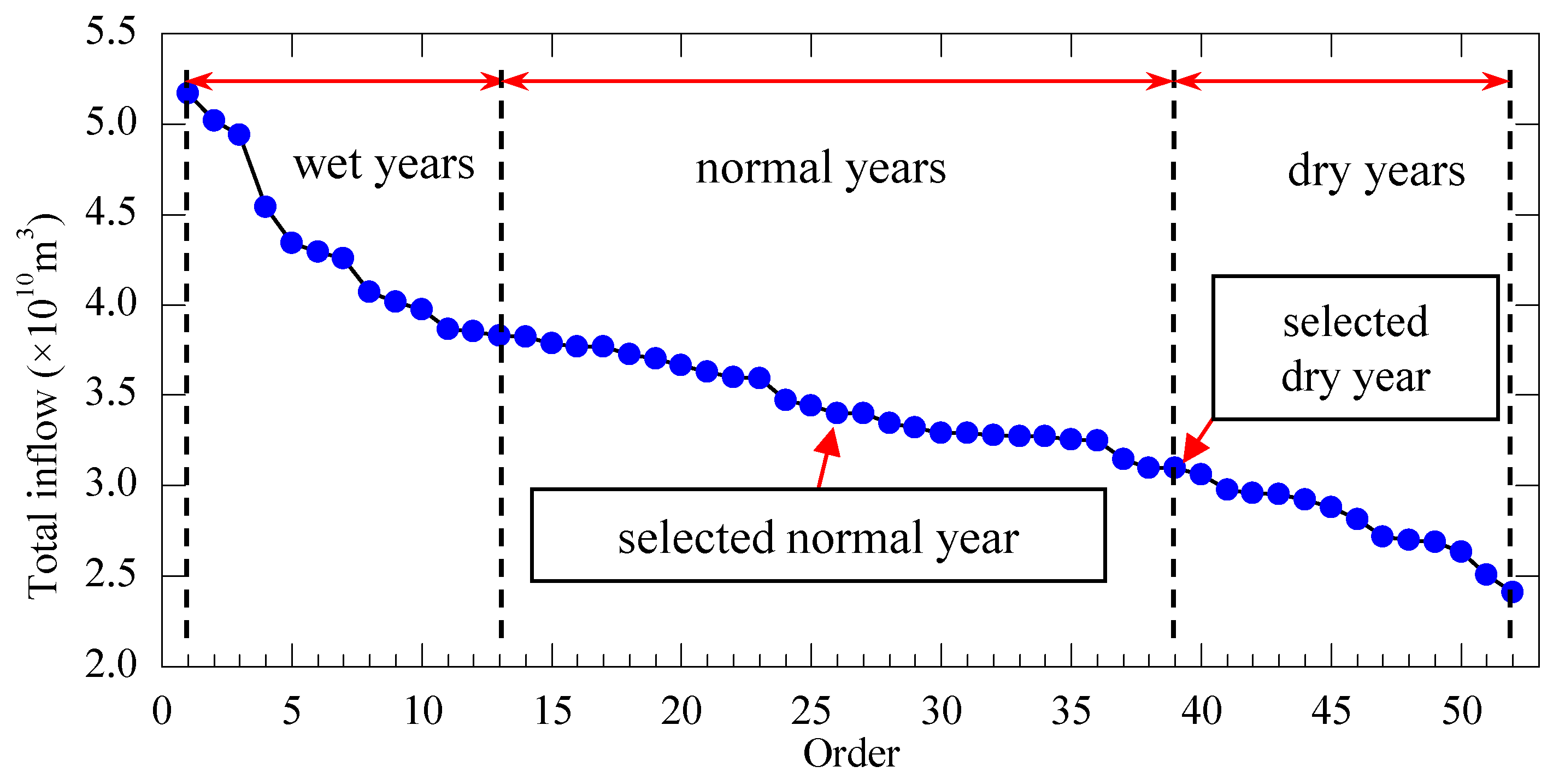
The optimal results strongly depend on the choice of the typical hydrological year, as inflows often vary widely among different regulatory years. Typical years include wet, normal and dry years. In this study, the inflow to the Xiluodu Reservoir in wet years is very high, in which case impoundment has little effect on the downstream environmental flow; thus, we selected a normal year and dry year as the typical years of interest. The Pingshan hydrological station is a controlled station in the lower reaches of the Jinsha River (Figure 1). Based on the daily average flow data of Pingshan station from 1956 to 2007 (52 years), the total flows during the impoundment period for every year were accumulated and ranked in descending order (Figure 4).
According to the definition of typical hydrological years in hydrology, the top 25% of the ranked total flows correspond to wet years, the total flows ranked between the top 25% and 75% correspond to normal years, and the total flows ranked below the top 75% correspond to dry years. Based on this principle, the typical dry year (ranked at 75%) and the typical normal year (ranked at 50%) were selected from among the dry years and the normal years, respectively. The inflows to the Xiluodu Reservoir in the corresponding typical years are shown in Figure 5.

3.2. Determination of the Appropriate Environmental Flow

The AEF concept was historically developed as a response to the degradation of aquatic ecosystems caused by human intervention [43,44]. The AEF is a crucial phenomenon in terms of electricity production and sustaining river integrity and is a key driver of ecological processes. Any flow disturbance may significantly affect and alter fluvial ecosystem dynamics [45,46].
More than 200 methods of determining environmental flows have been developed, and they can be classified into four principal groups: (1) hydrological methods [47,48], including the Tennant, 7Q10, flow duration curve (FDC), aquatic biological base flow, and RVA methods [49]; (2) hydraulic methods [50,51], including the wetted perimeter and R2CROSS methods; (3) habitat simulation methods [52], including the instream flow incremental methodology (IFIM), the physical habitat method, the weighted effective width method, and the minimum demand method for a biological space; and (4) holistic methods, including the building block method and benchmarking.
Currently, most AEFs obtained via either hydrological or hydraulic methods are calculated as fixed values which do not reflect the temporal variations in the river flow demand. For example, in the FDC method, only the flow value at a cumulative frequency of either 90% or 95% on the daily flow process curve is taken as the AEF, which is an approach that lacks practical rationality. To obtain an AEF that considers the temporal variations in demand, in this paper, the RVA method was used to calculate the AEF for the lower reaches of the Jinsha River. We calculated the AEF based on the runoff data collected at the Pingshan station from 1956 to 2007. The RVA method is a comprehensive method for assessing changes in river hydrological regimes by considering the size, frequency and variation characteristics of river flows. The calculation formula is as follows:
Q A E F , t = Q m e a n , t ( Q max , t Q min , t )
where Q A E F , t is the AEF in time step t , Q m e a n , t is the mean annual flow in time step t , and Q max , t and Q min , t are the maximum and minimum threshold values, respectively, in time step t as calculated using the RVA method.
The formulas for calculating the maximum and minimum threshold values are as follows:
Q max , t = max { ( 1 + μ ) Q m e d i a n , t , Q m e a n , t + μ Q s d , t } Q min , t = min { ( 1 η ) Q m e d i a n , t , Q m e a n , t μ Q s d , t }
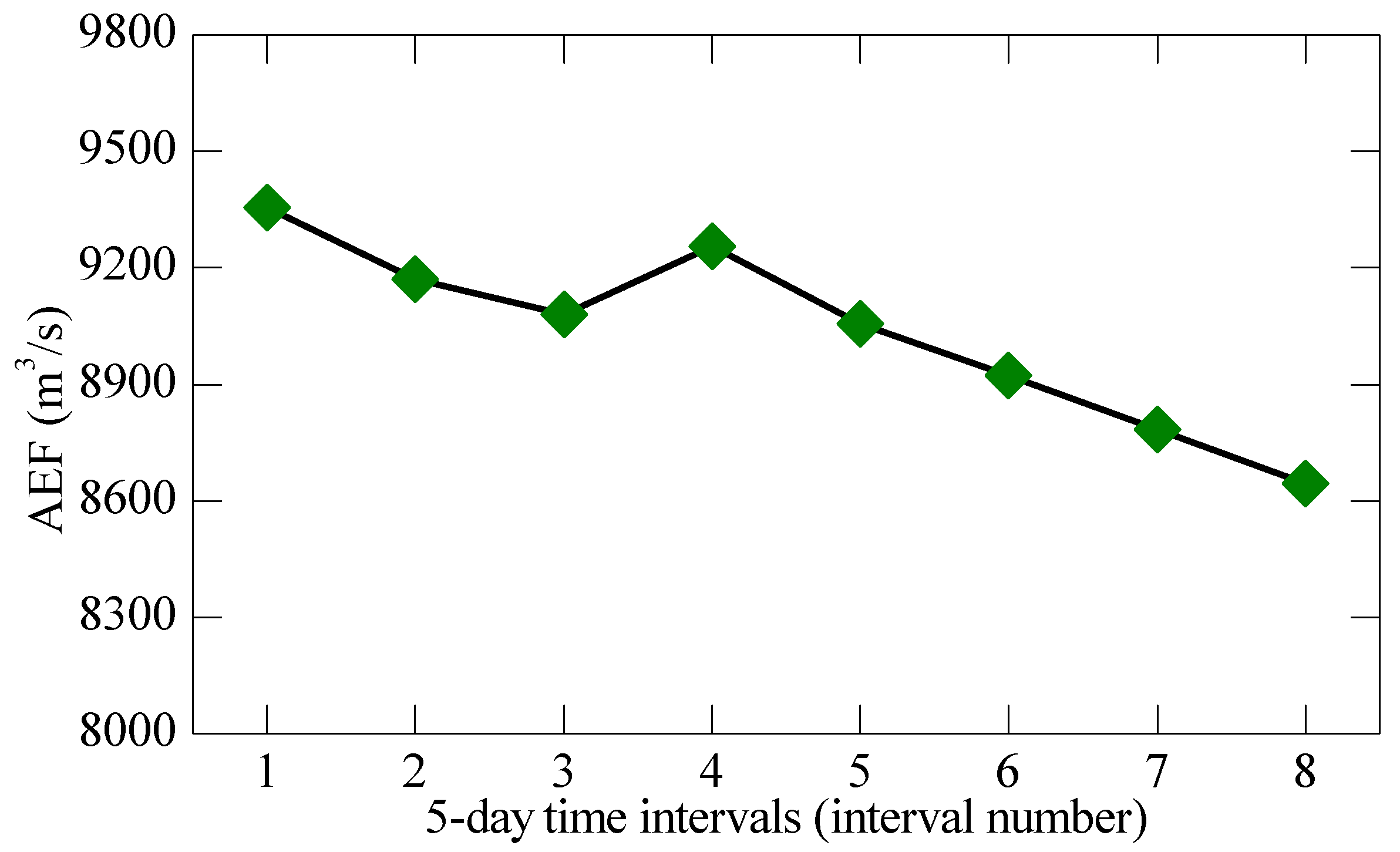
where η is a percentage that is generally equal to 17%; Q m e d i a n , t is the median flow in time step t; μ is an integer greater than 0, usually taken to be 1.0; and Q s d , t is the standard variance corresponding to the average flow in time step t . The AEF results calculated are plotted in Figure 6.

3.3. Optimization Results

3.3.1. Optimization Results for a Normal Year

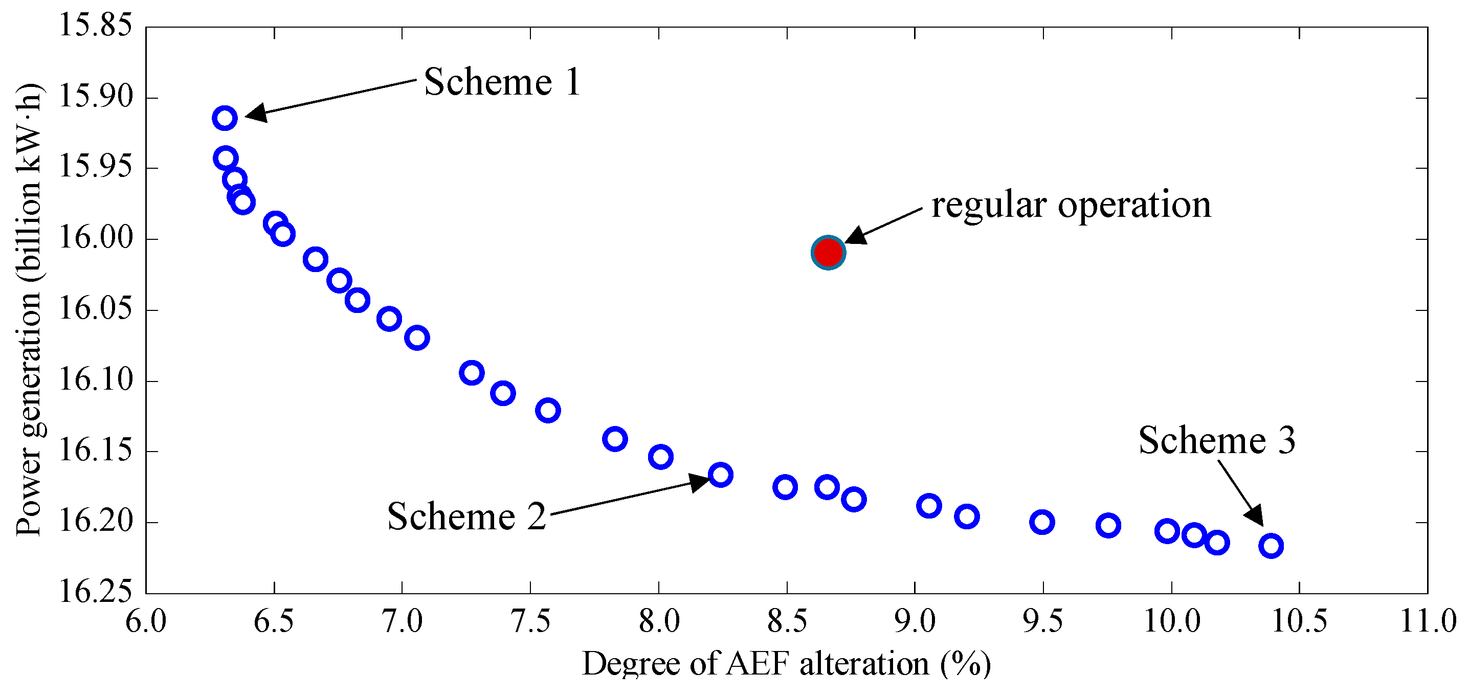
For the selected normal year, under the current regular operation policy, the total power generated by the cascade reservoir system during the impoundment period is 16.011 billion kW·h, and the degree of AEF alteration is 11.76%. The Pareto-optimal solution distribution for this normal year is shown in Figure 7. Three typical optimal schemes were selected for analysis of the reservoir water levels and outflows: scheme 1 (minimum degree of AEF alteration), scheme 2 (an unbiased optimal solution) and scheme 3 (maximum power generation). The red circle represents the reference scheme (regular operation). To achieve the maximum power generation, we can choose scheme 3, in which power generation is increased by 1.28% at the cost of increasing the degree of AEF alteration by 13.86%. To achieve the maximum ecological benefit, scheme 1 can be selected, in which the degree of AEF alteration is reduced by 22.53% with a 0.62% reduction in power generation. If there is no demand preference, we can choose scheme 2; while reducing the degree of AEF alteration by 6.38%, this scheme can also increase power generation by 0.89%. The details of these optimal results are shown in Table 2.
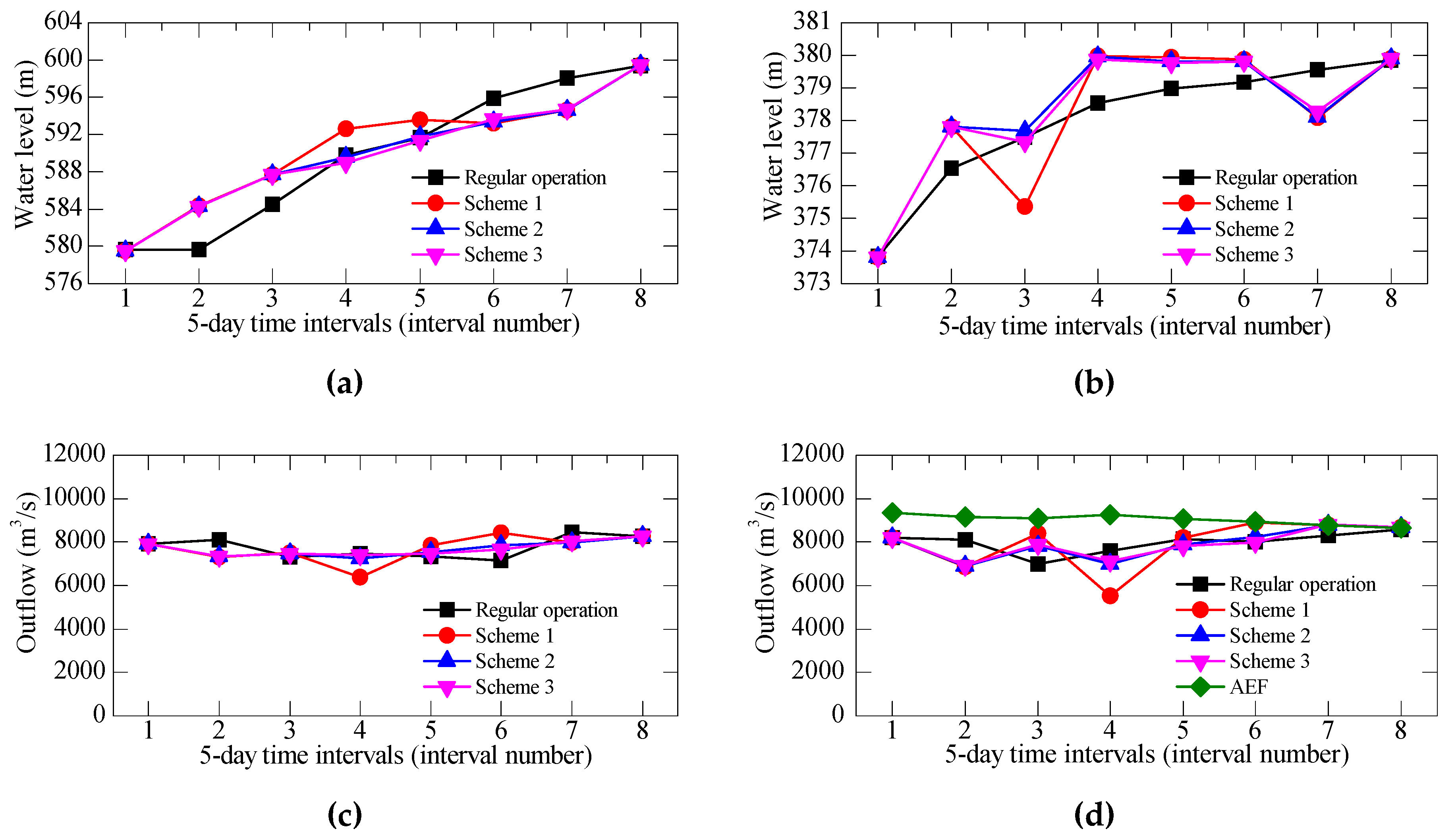
Figure 8 shows the cascade reservoir water levels and outflows for these three optimal schemes in a normal year. Under all three optimal schemes, the water storage capacity in the first two periods (intervals 1 and 2) is increased compared with that under regular operation, and the water level is increased earlier to enhance power generation. The water level of the Xiangjiaba Reservoir in the fourth period (interval 4) reaches 379.86 m and 379.85 m under schemes 3 and 2, respectively, and then remains at 379.80-379.90 m until the end of the water storage period under scheme 3. Considering the downstream environmental flow, under scheme 2, the outflow of the Xiangjiaba Reservoir is increased at the beginning of the seventh period (interval 7). To ensure that the downstream environmental water demand is met, in scheme 1, the outflow of the Xiangjiaba Reservoir is maintained as close as possible to the AEF; thus, the reservoir water level is slowly increased in the fourth and fifth periods. The Xiluodu Reservoir water level reaches 595.37 m in the 5th period; then, the outflow is increased in the seventh and eighth periods to meet the downstream environmental flow demand.

3.3.2. Optimization Results for a Dry Year

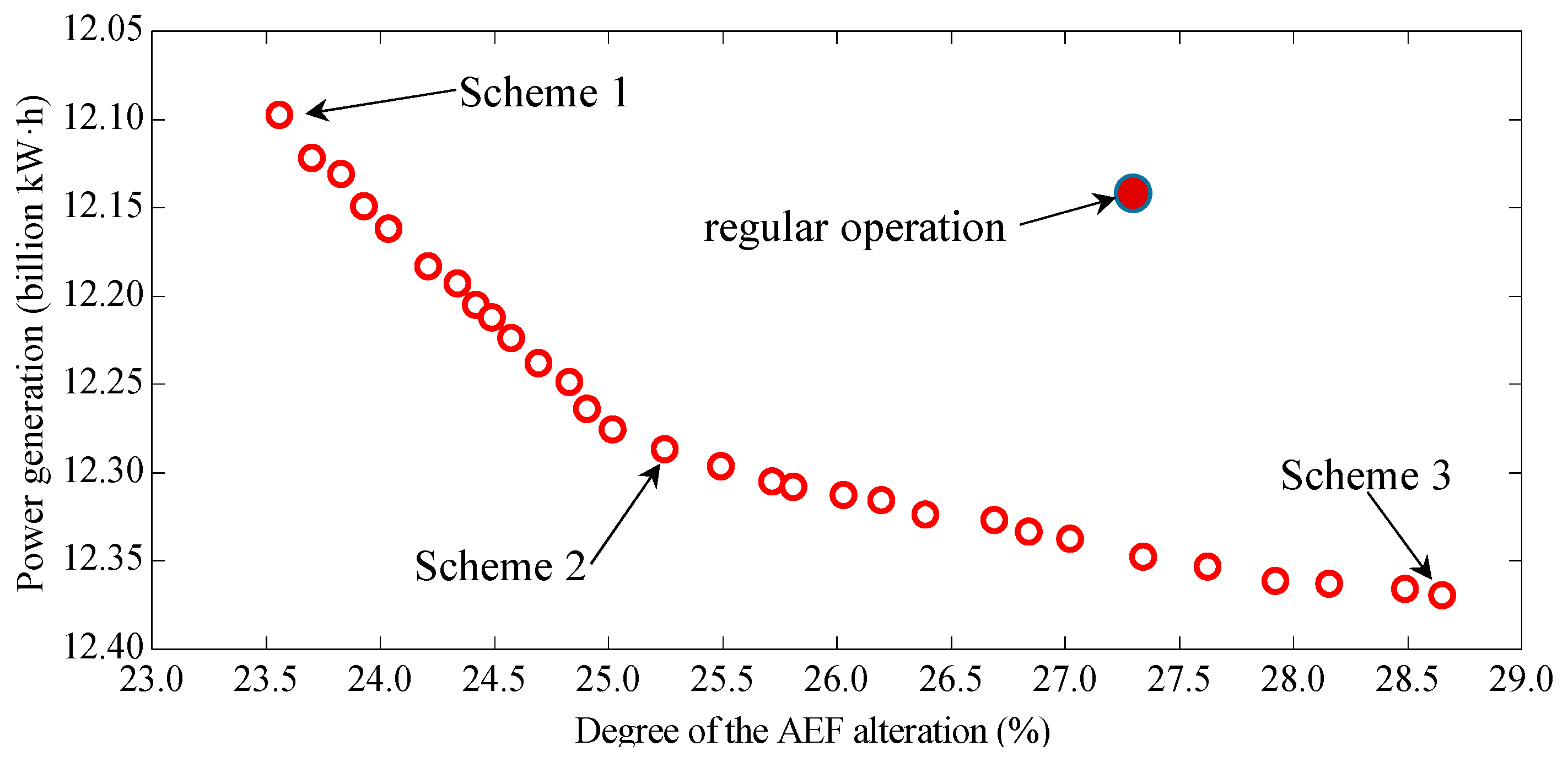
For the selected typical dry year, under the regular operation scheme, the total power generated by the cascade reservoir system during the impoundment period is 12.156 billion kW·h, and the degree of AEF alteration is 27.30%. The Pareto-optimal distribution for this dry year is shown in Figure 9. Again, three typical optimal schemes are selected, namely, scheme 1 (minimum degree of AEF alteration), scheme 2 (unbiased optimal solution), and scheme 3 (maximum power generation), to analyze the reservoir water levels and outflows. To maximize power generation, we can choose scheme 3, which increases power generation by 1.76% while increasing the degree of AEF alteration by 4.95%. To minimize the degree of AEF alteration, we can choose scheme 1, which reduces the degree of AEF alteration by 13.70% while decreasing power generation by 0.48%. If there is no demand preference, scheme 2 can increase power generation by 1.08% while decreasing the degree of AEF alteration by 7.51%. The details of the optimal results are shown in Table 3.
Figure 10 shows the cascade reservoir water levels and outflows for these three optimal schemes in a dry year. Due to the small inflow in dry years, the differences between the optimal schemes are smaller than those for a normal year. Under scheme 3, which prioritizes raising the water level, the Xiangjiaba Reservoir water level reaches 379.83 m in the fourth period and then remains above 379.00 m. The Xiluodu Reservoir water level reaches 599.36 m in the sixth period, and the water level is then decreased to 594.52 m in the seventh period to maintain a hydraulic head difference for power generation. In scheme 1, the outflow of the Xiluodu Reservoir begins to be increased in the fifth period to meet the demand for the downstream environmental flow. Compared to those in scheme 3, the average outflows of the Xiluodu Reservoir in the fifth and sixth periods in scheme 1 are increased by 775.46 m3/s and 817.27 m3/s, respectively. In both scheme 1 and scheme 2, the water level of the Xiluodu Reservoir is reduced in the seventh period so that the outflow is as close as possible to the AEF of the downstream river. In scheme 1, the average outflow to Xiangjiaba in the seventh period is 8481.55 m3/s, whereas in scheme 2, it is 8616.98 m3/s to meet the downstream AEF demand in the dry season.

3.4. Discussion

In the above analysis, operation optimization was performed for a typical normal hydrological year and a typical dry year, and three different optimal schemes and their levels of optimization were investigated for each typical year. For the typical normal year, the differences among the different optimal schemes are more obvious due to the larger inflow to the reservoirs. When the maximum power generation is sought, the water level of each reservoir increases quickly and then, once the highest water level is reached, it is maintained at this level for power generation. Therefore, the range of outflow fluctuation is large, leading to an increase in the environmental flow. By contrast, when the environmental flow is prioritized to minimize the degree of AEF alteration, the stability of the outflow must be maintained, resulting in a relatively slow rise in the reservoir water levels and, consequently, a reduction in the total power generation of the cascade reservoir system.
For the typical dry year, because the incoming flow is generally lower than the environmental flow, the differences among the various optimal schemes are smaller than those in the typical normal year. In the regular operation scheme, the reservoir water levels rise slowly. When the power generation is sought, the corresponding optimal scheme still gives priority to increasing the reservoir water levels as soon as possible, whereas when the goal is to minimize the degree of AEF alteration, the corresponding optimal scheme is designed to improve the ecological benefit of the cascade reservoir system by reducing the water levels during a certain period. In general, the optimal schemes obtained here are reasonably consistent with actual operations. During real operation, the manager can choose a suitable scheme in accordance with specific needs.

4. Conclusions

This paper establishes an optimal model for the impoundment period of the Xiangjiaba-Xiluodu cascade reservoir system considering both economic and ecological benefits, where the AEF of the downstream river is determined using the RVA method. In the proposed method, the improved INSGA2-DS algorithm is used as a viable means of determining the optimal reservoir scheduling by balancing objectives related to human needs, water management and river ecological protection. When the optimization is focused on maximizing economic benefit in a normal hydrological year and a dry year, the level of power generation can be increased by 1.28% and 1.76%, respectively, but the degree of change in the AEF is simultaneously increased by 13.86% and 4.95%, respectively (compared to the current regular operation scheme). Conversely, when the optimization is focused on ecological needs, the degree of AEF alteration can be reduced by 22.53% and 13.70%, respectively, while power generation is reduced by 0.62% and 0.48%, respectively. In addition, the wide distribution of the Pareto fronts produced using the proposed optimization techniques provides decision makers with considerable flexibility in establishing appropriate rules for reservoir operations by balancing human and ecological needs. The results not only verify the effectiveness of the proposed method but also provide a quantitative relationship between power generation and the degree of AEF alteration as well as operational references.

Author Contributions

Conceptualization, L.D. and H.D.; methodology, L.D. and Y.W.; software, Z.C. and C.M.; validation, L.D. and Z.C.; formal analysis, L.D.; investigation, J.G. and Z.C.; resources, H.D. and H.L.; data curation, L.D. and Z.C.; writing-original draft preparation, L.D.; writing—review and editing, L.D., C.M. and J.G.; supervision, H.D. and H.L. All authors have read and agreed to the published version of the manuscript.

Funding

This research was funded by the National Natural Science Foundation of China (51809150), the China Postdoctoral Science Foundation (2019T120119), the CRSRI Open Research Program (CKWV2019725/KY), and the Three Gorges Follow-up Research Project (2017HXXY-05).

Acknowledgments

The authors wish to acknowledge China Yangtze Power Corporation for the use of various facilities in carrying out this research. Many thanks are due to the anonymous referees for their detailed and helpful comments. In addition, the authors appreciate the review and editorial comments of the reviewers, and the editor.

Conflicts of Interest

The authors declare no conflict of interest.

References

  1. Zarei, A.; Mousavi, S.F.; Gordji, M.E.; Karami, H. Optimal Reservoir Operation Using Bat and Particle Swarm Algorithm and Game Theory Based on Optimal Water Allocation among Consumers. Water Resour. Manag. 2019, 33, 3071–3093. [Google Scholar] [CrossRef]
  2. Bilgili, M.; Bilirgen, H.; Ozbek, A.; Ekinci, F.; Demirdelen, T. The role of hydropower installations for sustainable energy development in Turkey and the world. Renew. Energy 2018, 126, 755–764. [Google Scholar] [CrossRef]
  3. Xu, B.; Ma, Y.F.; Zhong, P.A.; Yu, Z.B.; Zhang, J.Y.; Zhu, F.L. Bargaining Model of Synergistic Revenue Allocation for the Joint Operations of a Multi-Stakeholder Cascade Reservoir System. Water Resour. Manag. 2018, 32, 4625–4642. [Google Scholar] [CrossRef]
  4. Feng, Z.K.; Niu, W.J.; Cheng, C.T. China’s large-scale hydropower system: Operation characteristics, modeling challenge and dimensionality reduction possibilities. Renew. Energy 2019, 136, 805–818. [Google Scholar] [CrossRef]
  5. Zhou, Y.L.; Guo, S.L.; Chang, F.J.; Xu, C.Y. Boosting hydropower output of mega cascade reservoirs using an evolutionary algorithm with successive approximation. Appl. Energy 2018, 228, 1726–1739. [Google Scholar] [CrossRef]
  6. Neto, R.M.; Nocko, H.R.; Ostrensky, A. Environmental characterization and impacts of fish farming in the cascade reservoirs of the Paranapanema River, Brazil. Aquac. Environ. Interact. 2015, 6, 255–272. [Google Scholar]
  7. Yazdi, J.; Moridi, A. Multi-Objective Differential Evolution for Design of Cascade Hydropower Reservoir Systems. Water Resour. Manag. 2018, 32, 4779–4791. [Google Scholar] [CrossRef]
  8. Khorshidi, M.S.; Nikoo, M.R.; Sadegh, M.; Nematollahi, B. A Multi-Objective Risk-Based Game Theoretic Approach to Reservoir Operation Policy in Potential Future Drought Condition. Water Resour. Manag. 2019, 33, 1999–2014. [Google Scholar] [CrossRef]
  9. Graham, E.B.; Stegen, J.C.; Huang, M.; Chen, X.Y.; Scheibe, T.D. Subsurface biogeochemistry is a missing link between ecology and hydrology in dam-impacted river corridors. Sci. Total Environ. 2019, 657, 435–445. [Google Scholar] [CrossRef]
  10. Anindito, Y.; Haas, J.; Olivares, M.; Nowak, W.; Kern, J. A new solution to mitigate hydropeaking? Batteries versus re-regulation reservoirs. J. Clean Prod. 2019, 210, 477–489. [Google Scholar] [CrossRef]
  11. Al-Jawad, J.Y.; Alsaffar, H.M.; Bertram, D.; Kalin, R.M. Optimum socio-environmental flows approach for reservoir operation strategy using many-objectives evolutionary optimization algorithm. Sci. Total Environ. 2019, 651, 1877–1891. [Google Scholar] [CrossRef] [PubMed] [Green Version]
  12. Zhang, P.; Qiao, Y.; Schineider, M.; Chang, J.B.; Mutzner, R.; Fluixa-Sanmartin, J.; Yang, Z.; Fu, R.; Chen, X.J.; Cai, L.; et al. Using a hierarchical model framework to assess climate change and hydropower operation impacts on the habitat of an imperiled fish in the Jinsha River, China. Sci. Total Environ. 2019, 646, 1624–1638. [Google Scholar] [CrossRef] [PubMed]
  13. He, D.; Dai, Q.; Tang, H.; Yang, Z. Length-weight relationships for three fish species from the middle and lower reaches of the Jinsha River, China. J. Appl. Ichthyol. 2018, 34, 760–761. [Google Scholar] [CrossRef]
  14. Shao, K.; Que, Y.F.; Xiong, M.H.; Li, W.T.; Yu, D.; Shi, F. Length-weight and length-length relationships of thirteen fish species from the lower Jinsha River, southwest China. J. Appl. Ichthyol. 2018, 34, 774–776. [Google Scholar] [CrossRef]
  15. Zhang, P.; Cai, L.; Yang, Z.; Chen, X.J.; Qiao, Y.; Chang, J.B. Evaluation of fish habitat suitability using a coupled ecohydraulic model: Habitat model selection and prediction. River Res. Appl. 2018, 34, 937–947. [Google Scholar] [CrossRef]
  16. Li, G.N.; Sun, S.K.; Liu, H.T.; Zheng, T.G. Optimizing the entrance location for a fish pass facility with limited attraction flow in a large river—A case study of the Jinsha River, China. Can. J. Civ. Eng. 2019, 46, 847–857. [Google Scholar] [CrossRef]
  17. Luo, D.N.; Lin, P.; Li, Q.B.; Zheng, D.; Liu, H.Y. Effect of the impounding process on the overall stability of a high arch dam: A case study of the Xiluodu dam, China. Arab. J. Geosci. 2015, 8, 9023–9041. [Google Scholar] [CrossRef]
  18. Zhu, T.B.; Yang, D.G. Length-weight relationships of two fish species from the middle reaches of the Jinsha River, China. J. Appl. Ichthyol. 2016, 32, 747–748. [Google Scholar] [CrossRef]
  19. Morrison, R.R.; Stone, M.C. Evaluating the impacts of environmental flow alternatives on reservoir and recreational operations using system dynamics modeling. J. Am. Water Resour. Assoc. 2015, 51, 33–46. [Google Scholar] [CrossRef]
  20. Karakoyun, Y.; Donmez, A.H.; Yumurtaci, Z. Comparison of environmental flow assessment methods with a case study on a runoff river-type hydropower plant using hydrological methods. Environ. Monit. Assess. 2018, 190, 1–15. [Google Scholar] [CrossRef]
  21. Rashid, M.U.; Latif, A.; Azmat, M. Optimizing Irrigation Deficit of Multipurpose Cascade Reservoirs. Water Resour. Manag. 2018, 32, 1675–1687. [Google Scholar] [CrossRef]
  22. King, A.J.; Gawne, B.; Beesley, L.; Koehn, J.D.; Nielsen, D.L.; Price, A. Improving Ecological Response Monitoring of Environmental Flows. Environ. Manag. 2015, 55, 991–1005. [Google Scholar] [CrossRef] [PubMed]
  23. Giraldo, M.A.; Dark, S.; Pendleton, P.; Stein, E.D.; Mazor, R.; Andreas, J. Environmental predictors of stream flow in semi-arid watersheds for biological assessments. Ecol. Indic. 2019, 104, 429–438. [Google Scholar] [CrossRef]
  24. Dupuis, J.R.; Cullingham, C.I.; Nielsen, S.E.; Sperling, F.A.H. Environmental effects on gene flow in a species complex of vagile, hilltopping butterflies. Biol. J. Linnean Soc. 2019, 127, 417–428. [Google Scholar] [CrossRef]
  25. Zhang, H.X.; Chang, J.X.; Gao, C.; Wu, H.S.; Wang, Y.M.; Lei, K.X.; Long, R.H.; Zhang, L.P. Cascade hydropower plants operation considering comprehensive ecological water demands. Energy Conv. Manag. 2019, 180, 119–133. [Google Scholar] [CrossRef]
  26. Takada, A.; Hiramatsu, K.; Trieu, N.A.; Harada, M.; Tabata, T. Development of an optimizing method for the operation rule curves of a multipurpose reservoir in a Southeast Asian watershed. Paddy Water Environ. 2019, 17, 195–202. [Google Scholar] [CrossRef]
  27. Sichilalu, S.; Wamalwa, F.; Akinlabi, E.T. Optimal control of wind-hydrokinetic pumpback hydropower plant constrained with ecological water flows. Renew. Energy 2019, 138, 54–69. [Google Scholar] [CrossRef]
  28. Stuart, I.; Sharpe, C.; Stanislawski, K.; Parker, A.; Mallen-Cooper, M. From an irrigation system to an ecological asset: Adding environmental flows establishes recovery of a threatened fish species. Mar. Freshw. Res. 2019, 70, 1295–1306. [Google Scholar] [CrossRef] [Green Version]
  29. Lu, P.; Zhou, J.Z.; Wang, C.; Qiao, Q.; Mo, L. Short-term hydro generation scheduling of Xiluodu and Xiangjiaba cascade hydropower stations using improved binary-real coded bee colony optimization algorithm. Energy Conv. Manag. 2015, 91, 19–31. [Google Scholar] [CrossRef]
  30. Geressu, R.T.; Harou, J.J. Reservoir system expansion scheduling under conflicting interests. Environ. Modell. Softw. 2019, 118, 201–210. [Google Scholar] [CrossRef]
  31. Yassin, F.; Razavi, S.; Elshamy, M.; Davison, B.; Sapriza-Azuri, G.; Wheater, H. Representation and improved parameterization of reservoir operation in hydrological and land-surface models. Hydrol. Earth Syst. Sci. 2019, 23, 3735–3764. [Google Scholar] [CrossRef] [Green Version]
  32. Fallah-Mehdipour, E.; Bozorg-Haddad, O.; Loaiciga, H.A. Calculation of multi-objective optimal tradeoffs between environmental flows and hydropower generation. Environ. Earth Sci. 2018, 77, 1–10. [Google Scholar] [CrossRef]
  33. Carmignani, J.R.; Roy, A.H. Ecological impacts of winter water level drawdowns on lake littoral zones: A review. Aquat. Sci. 2017, 79, 803–824. [Google Scholar] [CrossRef] [Green Version]
  34. Xie, M.F.; Zhou, J.Z.; Li, C.L.; Zhu, S. Long-term generation scheduling of Xiluodu and Xiangjiaba cascade hydro plants considering monthly streamflow forecasting error. Energy Conv. Manag. 2015, 105, 368–376. [Google Scholar] [CrossRef]
  35. Shen, J.J.; Zhang, X.F.; Wang, J.; Cao, R.; Wang, S.; Zhang, J.H. Optimal Operation of Interprovincial Hydropower System Including Xiluodu and Local Plants in Multiple Recipient Regions. Energies 2019, 12, 144. [Google Scholar] [CrossRef] [Green Version]
  36. Kamodkar, R.U.; Regulwar, D.G. Optimal multiobjective reservoir operation with fuzzy decision variables and resources: A compromise approach. J. Hydro-Environ. Res. 2014, 8, 428–440. [Google Scholar] [CrossRef]
  37. Shahhosseini, H.R.; Farsi, M.; Eini, S. Multi-objective optimization of industrial membrane SMR to produce syngas for Fischer-Tropsch production using NSGA-II and decision makings. J. Nat. Gas Sci. Eng. 2016, 32, 222–238. [Google Scholar] [CrossRef]
  38. Navabi, S.; Khaninezhad, R.; Jafarpour, B. A unified formulation for generalized oilfield development optimization. Comput. Geosci. 2017, 21, 47–74. [Google Scholar] [CrossRef]
  39. Prakash, O.; Srinivasan, K.; Sudheer, K.P. Adaptive multi-objective simulation-optimization framework for dynamic flood control operation in a river-reservoir system. Hydrol. Res. 2015, 46, 893–911. [Google Scholar] [CrossRef]
  40. Peng, S.T.; Li, T.; Zhao, J.L.; Lv, S.P.; Tan, G.Z.; Dong, M.M.; Zhang, H.C. Towards energy and material efficient laser cladding process: Modeling and optimization using a hybrid TS-GEP algorithm and the NSGA-II. J. Clean Prod. 2019, 227, 58–69. [Google Scholar] [CrossRef]
  41. Mann, G.W.; Eckels, S. Multi-objective heat transfer optimization of 2D helical micro-fins using NSGA-II. Int. J. Heat Mass Transf. 2019, 132, 1250–1261. [Google Scholar] [CrossRef]
  42. Jadidi, A.; Menezes, R.; de Souza, N.; de Castro Lima, A.C. Short-Term Electric Power Demand Forecasting Using NSGA II-ANFIS Model. Energies 2019, 12, 1891. [Google Scholar] [CrossRef] [Green Version]
  43. Grantham, T.E.; Zimmerman, J.K.H.; Carah, J.K.; Howard, J.K. Stream flow modeling tools inform environmental water policy in California. Calif. Agric. 2019, 73, 33–39. [Google Scholar] [CrossRef]
  44. Zhao, C.S.; Yang, S.T.; Liu, J.G.; Liu, C.M.; Hao, F.H.; Wang, Z.G.; Zhang, H.T.; Song, J.X.; Mitrovic, S.M.; Lim, R.P. Linking fish tolerance to water quality criteria for the assessment of environmental flows: A practical method for streamflow regulation and pollution control. Water Res. 2018, 141, 96–108. [Google Scholar] [CrossRef]
  45. Ceola, S.; Pugliese, A.; Ventura, M.; Galeati, G.; Montanari, A.; Castellarin, A. Hydro-power production and fish habitat suitability: Assessing impact and effectiveness of ecological flows at regional scale. Adv. Water Resour. 2018, 116, 29–39. [Google Scholar] [CrossRef]
  46. Theodoropoulos, C.; Skoulikidis, N.; Rutschmann, P.; Stamou, A. Ecosystem-based environmental flow assessment in a Greek regulated river with the use of 2D hydrodynamic habitat modelling. River Res. Appl. 2018, 34, 538–547. [Google Scholar] [CrossRef]
  47. Ksiazek, L.; Wos, A.; Florek, J.; Wyrebek, M.; Mlynski, D.; Walega, A. Combined use of the hydraulic and hydrological methods to calculate the environmental flow: Wisloka river, Poland: Case study. Environ. Monit. Assess. 2019, 191, 1–17. [Google Scholar] [CrossRef] [Green Version]
  48. Mishra, S.K.; Amrit, K.; Pandey, R.P. Correlation between Tennant method and Standardized Precipitation Index for predicting environmental flow condition using rainfall in Godavari Basin. Paddy Water Environ. 2019, 17, 515–521. [Google Scholar] [CrossRef]
  49. Windfeld, E.J.; Ford, J.D.; Berrang-Ford, L.; McDowell, G. How do community-level climate change vulnerability assessments treat future vulnerability and integrate diverse datasets? A review of the literature. Environ. Rev. 2019, 27, 427–434. [Google Scholar] [CrossRef]
  50. El-Jabi, N.; Caissie, D. Characterization of natural and environmental flows in New Brunswick, Canada. River Res. Appl. 2019, 35, 14–24. [Google Scholar] [CrossRef] [Green Version]
  51. Vietz, G.J.; Lintern, A.; Webb, J.A.; Straccione, D. River Bank Erosion and the Influence of Environmental Flow Management. Environ. Manag. 2018, 61, 454–468. [Google Scholar] [CrossRef] [PubMed]
  52. Johnson, J.A.; Sivakumar, K.; Rosenfeld, J. Ecological flow requirement for fishes of Godavari river: Flow estimation using the PHABSIM method. Curr. Sci. 2017, 113, 2187–2193. [Google Scholar] [CrossRef]
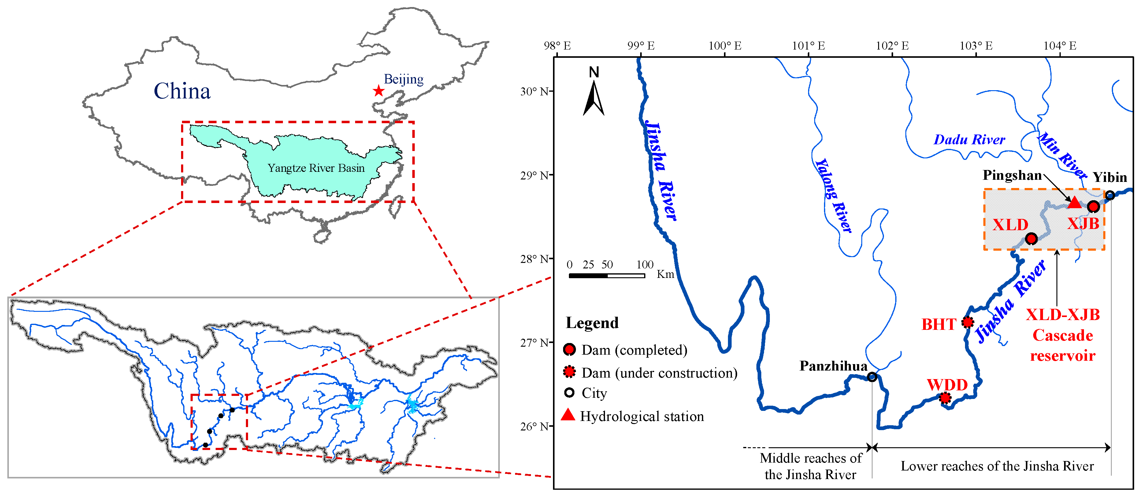
Figure 1. Location of the Xiluodu-Xiangjiaba cascade reservoir system.
Sustainability 12 00966 g001
Figure 2. Flowchart of the INSGA2-DS procedure.
Sustainability 12 00966 g002
Figure 3. Solution process for using INSGA2-DS to optimize cascade reservoir operation.
Sustainability 12 00966 g003
Figure 4. Diagram ranking each year by the total flow during the impoundment period.
Sustainability 12 00966 g004
Figure 5. Inflows to Xiluodu Reservoir in the different typical years.
Sustainability 12 00966 g005
Figure 6. Appropriate environmental flow (AEF) in the lower reaches of the Jinsha River.
Sustainability 12 00966 g006
Figure 7. Pareto-optimal distribution for a normal year.
Sustainability 12 00966 g007
Figure 8. Reservoir water levels and outflows under different typical schemes in a normal year: (a) water level of the Xiluodu Reservoir; (b) water level of the Xiangjiaba Reservoir; (c) outflow of the Xiluodu Reservoir; (d) outflow of the Xiangjiaba Reservoir.
Sustainability 12 00966 g008
Figure 9. Pareto-optimal distribution for a dry year.
Sustainability 12 00966 g009
Figure 10. Reservoir water levels and outflows under different optimal schemes in a dry year: (a) water level of the Xiluodu Reservoir; (b) water level of the Xiangjiaba Reservoir; (c) outflow of the Xiluodu Reservoir; (d) outflow of the Xiangjiaba Reservoir.
Sustainability 12 00966 g010aSustainability 12 00966 g010b
Table 1. Main parameters of the Xiluodu-Xiangjiaba cascaded hydropower stations.
ParameterXiluodu ReservoirXiangjiaba Reservoir
Height of dam (m)285.5162.0
Dead water level (m)540.0370.0
Normal water level (m)600.0380.0
Flood limit water level (m)560.0370.0
Installed capacity (MW)126006000
Minimum output (MW)66502000
Maximum output (MW)126006000
Total capacity (108 m3)126.751.6
Minimum outflow (m3/s)15001500
Table 2. Optimal results under three typical schemes in normal year.
SchemeObjectivePower Generation
(Billion kW·h)
Degree of AEF Alteration (%)
Scheme 1Minimizing the degree of AEF alteration15.9129.11%
Scheme 2Unbiased16.15311.01%
Scheme 3Maximizing the power generation16.21713.39%
Reference schemeRegular operation16.01111.76%
Table 3. Optimal results under three typical schemes in a dry year.
SchemeObjectivePower Generation
(billion kW·h)
Degree of the AEF Alteration (%)
Scheme 1Minimizing the degree of AEF alteration12.09823.56%
Scheme 2Unbiased12.28725.25%
Scheme 3Maximizing the power generation12.37028.65%
Reference scheme Regular operation12.15627.30%