Revising Seismic Vulnerability of Bridges Based on Bayesian Updating Method to Evaluate Traffic Capacity of Bridges

Abstract

Analyzing the seismic vulnerability of bridge structures is of great significance in assessing the sustainable capacity of bridges. However, previous seismic vulnerability analysis of bridge structures was based on theoretical simulation or experimental research, which couldn’t really reflect the actual seismic damage. Therefore, this paper used Bayesian updating method to obtain a corrected vulnerability curve of bridge structures considering the theoretical simulation and historical seismic data, which overcame the shortcomings that information couldn’t be updated. Specifically speaking, the seismic demand probability function of the bridge structure was obtained through numerical simulation, and a seismic vulnerability curve of a log-normal distribution with two parameters (median value $c_j$ and log-standard deviation ${\xi }_j$) was established, which was taken as the prior information. Then, combining the historical empirical damage data, the demand information is updated to obtain the posterior probability of the structural seismic demand. The possibility of exceeding the limit damage state of the bridge structure under different ground motion intensity can be obtained by using the corrected seismic vulnerability curve. The results show that the corrected seismic vulnerability curves are closer to theoretical simulation results, which provides a new idea for the reliability analysis of the bridge structure. Moreover, based on the corrected seismic vulnerability curve of Guxigou Middle Bridge, the post-earthquake traffic capacity of the bridge was evaluated by combining with traffic flow and traffic time. The research results show that the proposed method can quickly evaluate the sustainable traffic capacity of bridges after earthquakes, which has certain practicability and scientificity and provides the theoretical basis and practical guiding significance for the relief work after earthquakes.

1. Introduction

In recent years, frequent earthquakes have resulted in huge economic loss and severe social impact on people’s life. As an important part of the traffic lifeline project, bridges are widely distributed and are easily damaged by earthquakes. After the earthquake, many bridges will be directly damaged, which not only brings many problems to social life and economic operation, but also causes great difficulties in rescue and relief work after the earthquake. Therefore, analyzing the sustainable traffic capacity of bridges under earthquake disaster conditions is very important for emergency decision-making of traffic lifeline systems [1]. The Transportation Research Board (TRB) published the first edition of “Highway Capacity Manual (HCM)” [2] in 1950, which defined the concept of capacity. Most previous researches on the traffic capacity of bridges mainly relied on monitoring the health state of bridge structures. Cabboi et al. [3] proposed an automated procedure based on parametric identification methods for health monitoring for bridge structures. Chalouhi et al. [4] presented a novelty detection method for railway bridges, and based on a small a priori probability of anomaly in the bridge, the conditional/posterior probability of anomaly was computed by using the Bayesian inference. As we all know, the reliability of the bridge structures after earthquakes will directly affect the sustainable traffic capacity of bridges. However, effective disaster risk management strategies and practices depend on a rigorous understanding of the dimensions of exposure and vulnerability [5]. Barbat et al. [6] proposed seismic vulnerability and risk evaluation methods for urban areas considering the influence of multiple factors. Chieffo et al. [7] proposed that the seismic risk assessment is a multivariate problem based on the estimation of three major factors such as vulnerability, exposure, and hazard. In previous studies, seismic vulnerability analysis has been widely used in seismic reliability analysis of structures [8,9].

At present, the analysis of seismic performance of bridges under different working conditions usually takes the form of seismic vulnerability curves [10,11,12,13]. An empirical and theoretical method was used to construct the seismic vulnerability curves by researchers [14,15]. Laura et al. [16] used operational modal analysis and experimental modal analysis to compare with the numerical model, which was used to evaluate the load bearing capacity and structural behavior of a viaduct under traffic or seismic excitation. Zani et al. [17] built a detailed 3D finite-element (FE) model to analyze the seismic behavior of the Azzone Visconti Bridge by using nonlinear dynamic analysis method. According to Cornell’s research [18], seismic demand and ground motion parameters–ground motion peak ground acceleration (PGA) followed the log-normal distribution. California Department of Transportation classified the damage states of bridge structures into five categories, including no damage (ND), slight damage (SD), moderate damage (MD), extensive damage (ED), and complete damage (CD) [19]. Shinozuka et al. [20] built the empirical vulnerability curve based on bridge damage data in the Kobe earthquake. Hwang et al. [21] used a displacement ductility ratio of piers as a damage degree to define the damage levels of the bridge, and the seismic vulnerability curves under four damage states were obtained. Choi et al. [22] established a theoretical seismic vulnerability curve for bridge structures in the mid-earthquake region. Duan et al. [23] proposed a modified coefficient model to evaluate the traffic capacity of the rescue road after the earthquake. Lan et al. [24] established the seismic vulnerability curves of beam bridges and arch bridges based on the damage data and proposed a method for evaluating the traffic capacity of common bridges after the earthquake. Liu [25] proposed a method for assessing the overall impact of the seismic vulnerability of urban bridges on the transportation network. However, all these methods have their deficiencies. Although the results of empirical analysis method are credible, these results are limited by lack of enough seismic information in most areas [26]. While the theoretical analysis method is used to develop the seismic vulnerability curve of bridge structures, it is conducted only through nonlinear analysis of the bridge structure. In addition, the information obtained through the above methods cannot be updated in a timely manner. Therefore, this study established firstly a seismic vulnerability curve of the logarithmic normal distribution with two parameters (median value $c_j$ and log-standard deviation ${\xi }_j$) based on the numerical simulation. Based on Bayesian updating method, combining the historical empirical damage data, the theoretical simulation results were taken as the prior information to update the seismic demand information of bridge structures. Finally, a corrected seismic vulnerability curve of bridges was drawn to evaluate the damage states of bridge structures under different ground motion intensity. Moreover, the sustainable traffic capacity of bridges after the earthquake was evaluated based on the corrected seismic vulnerability curve.

2. Seismic Vulnerability Analysis of Bridge

Based on existing research [18,27,28,29,30,31], it is assumed that the probability distribution model of the seismic vulnerability curves can be expressed in the form of lognormal distribution function with two parameter (median value $c_j$ and log-standard deviation ${\xi }_j$), and the maximum likelihood method was used to estimate these two parameters.

$$P_f=\mathrm{F}\left(a_i;c_j,{\xi }_j\right)=\Phi (\frac{\ln (a_i/c_j)}{{\xi }_j})$$

(1)

where, $\mathrm{F}(a_i;c_j,{\xi }_j)$ is the seismic vulnerability curve of the i-th bridge under the damage state j. $a_i$ is the peak ground acceleration (PGA) of the i-th bridge.

The likelihood function is expressed as follows:

$$\mathrm{L}={\displaystyle \prod }_{i=1}^N[[\mathrm{F}\left(a_i;c_j,{\xi }_j\right){]}^{x_i}{[1-\mathrm{F}\left(a_i;c_j,{\xi }_j\right)]}^{1-x_i}]$$

(2)

where, $x_i$ is a Boolean random variable of a given damage state of the i-th bridge at $a_i$.

The maximum likelihood estimations of two parameters can be obtained by solving the following equation [18,29,32,33,34]:

$$\frac{\partial lnL}{\partial c_j}=\frac{\partial lnL}{\partial \xi }=0$$

(3)

Two parameters of the seismic vulnerability curve calculated by this method are brought into Equation (1) to establish the seismic vulnerability curves under different damage states.

3. Bayesian Parameter Estimation Method

3.1. Bayesian Method Principle

According to probability theory and multiplication law [35], the probability of the product of two random variables is as follows:

$$p\left(\frac{\theta }{\epsilon }\right)=\frac{\left[p\left(\frac{\epsilon }{\theta }\right)p\left(\theta \right)\right]}{p\left(\epsilon \right)}$$

(4)

According to the total probability formula, if random variable $\epsilon$ is consisted of many unrelated events, there is:

$$p\left(\epsilon \right)={\displaystyle \sum }_{i}p\left(\epsilon /\theta \right)/p\left(\theta \right)$$

(5)

Bayesian theorem is obtained by bringing Equation (5) into Equation (4):

$$p\left(\theta /\epsilon \right)=\left[p\left(\frac{\epsilon }{\theta }\right)p\left(\theta \right)\right]{\displaystyle \sum }_{i}p\left(\epsilon /\theta \right)/p\left(\theta \right)$$

(6)

where, $p\left(\theta /\epsilon \right)$ is the posterior probability of parameter $\theta$, $p\left(\theta \right)$ is the prior probability of parameter $\theta$. The Bayesian theorem is expressed that the posterior probability of a random variable is the product of its prior probability, likelihood function, and normalization constant.

3.2. Parameter Estimation Method

Bayesian parameter estimation method uses prior distribution information (that is, numerical simulation) to make a preliminary estimation of the parameter distribution probability model. Then, based on the posterior data, which is historical empirical damage data of bridge structures, the probability distribution parameters are re-estimated and updated to make full use of existing data.

Due to the seismic demand and ground motion parameters–ground motion peak ground acceleration (PGA) follow the log-normal distribution [18], suppose that $f\left(x\right)$ is a lognormal distribution density function of random variable $x$. $\mu$ and $\sigma$ are the median value and standard deviation of data samples ($ln{x}_1,ln{x}_2,\dots ,\ln x_n$) based on seismic damage tests or theoretical simulation of $n$ bridges, respectively. ${\mu }^{\prime }$ and ${\sigma }^{\prime }$ are the median value and standard deviation of statistical samples ($ln{x}_1,ln{x}_2,\dots ,\ln x_m$) based on historical bridge earthquake damage of $m$ bridges, respectively. If the prior distribution of μ is a lognormal function that is $f^{\prime \left(\mu \right)}~LN\left({\mu }^{\prime }, {\sigma }^{\prime }\right)$, the posterior distribution $f^{″}\left(\mu \right)$ of $\mu$ is expressed as follows [36,37,38]:

$$f^{″}\left(\mu \right)=\frac{\left[{{\displaystyle \prod }}_{i=1}^{n}f\left(x_i|\mu \right)dx\right]·f^{\prime }\left(\mu \right)}{{{\displaystyle \int }}_{-\infty }^{\infty }\left[{{\displaystyle \prod }}_{i=1}^{n}f\left(x_i|\mu \right)dx\right]·f^{\prime }\left(\mu \right)du}~LN\left({\mu }^{″},{\sigma }^{″}\right)$$

(7)

According to Bayesian principle, two posterior lognormal distribution parameters (median value ${\mu }^{″}$ and standard deviation ${\sigma }^{″}$) of the random variable x can be expressed as follows:

$${\mu }^{″}=\frac{\mu ·\frac{{\left({\sigma }^{\prime }\right)}^2}{m}+{\mu }^{\prime }·\frac{\left({\sigma }^2\right)}{n}}{\frac{{\left({\sigma }^{\prime }\right)}^2}{m}+\left(\frac{{\sigma }^2}{n}\right)}$$

(8)

$${\sigma }^{″}=\sqrt{\frac{\left(m+n\right){\left({\sigma }^{\prime }\right)}^2·\frac{{\sigma }^2}{m·n}}{\frac{{\left({\sigma }^{\prime }\right)}^2}{m}+\left(\frac{{\sigma }^2}{n}\right)}}$$

(9)

So far, the median value ${\mu }^{″}$ and standard deviation ${\sigma }^{″}$ based on Bayesian updating method are the two parameters (median value $c_j$ and log-standard deviation ${\xi }_j$) of Equations (1)–(3).

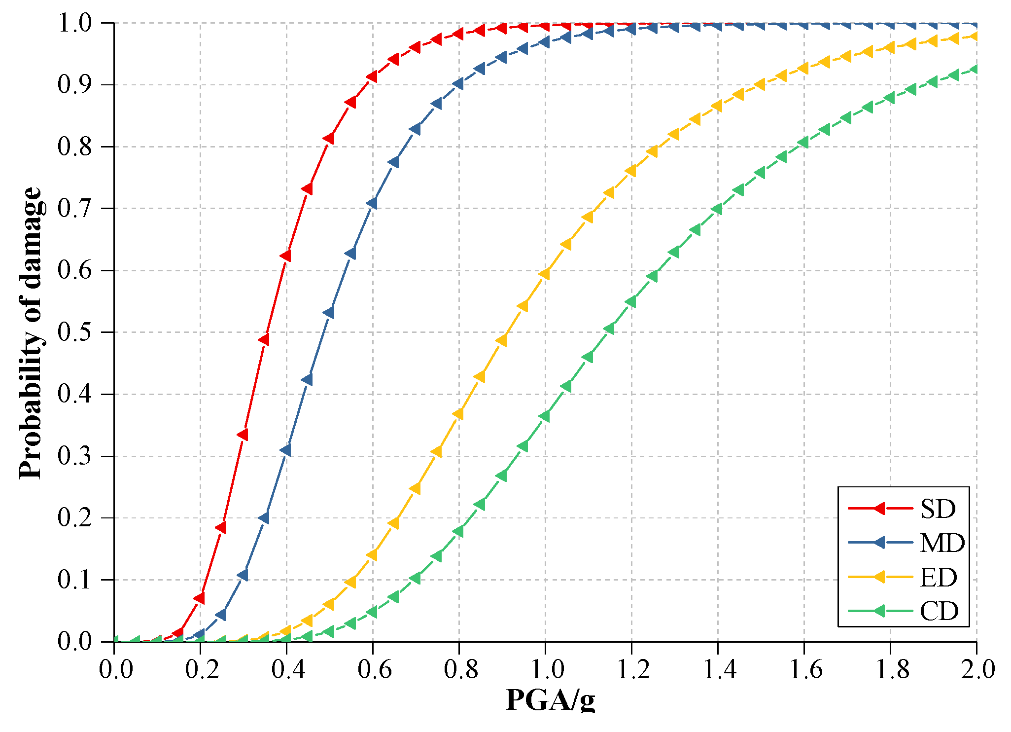
4. Seismic Vulnerability Curves Based on Historical Damage Data

At 14:18 on May 12, 2008, a magnitude 8.0M earthquake occurred Yingxiu, Wenchuan country, Sichuan province, China. Plenty of bridges suffered damage in the western area of Sichuan province. Lin [39] comprehensively investigated the seismic damage situation in the Wenchuan earthquake. By using these data and other supplementary data obtained from surveys, a total of 2150 bridges were finally sorted out, including 611 arc bridges and 1539 girder bridges. According to damage level, the damage states of these bridges were divided into four categories, including slight damage (SD), moderate damage (MD), extensive damage (ED), and complete damage (CD).

Due to the damage data include the structural vulnerability factors and uncertainty factors, the calculated seismic vulnerability curves (Figure 1) are reasonable and reliable.

Table 1. The seismic vulnerability curve parameters based on historical damage data.

Damage State	Girder Bridge Parameters		Arch Bridge Parameters
	$\mathbf{Median} \mathbf{Value} {\mathit{c}}_{\mathit{j}}$	$\mathbf{Log}\text{-}\mathbf{Standard} \mathbf{Deviation} {\mathit{\xi }}_{\mathit{j}}$	$\mathbf{Median} \mathbf{Value} {\mathit{c}}_{\mathit{j}}$	$\mathbf{Log}\text{-}\mathbf{Standard} \mathbf{Deviation} {\mathit{\xi }}_{\mathit{j}}$
SD	0.224	1.002	0.237	1.003
MD	0.583	0.752	0.459	0.887
ED	1.192	0.701	0.866	0.836
CD	1.864	0.661	2.019	0.804

shows two parameters of the logarithmic normal distribution [39]. By counting the damage degree of different bridges during Wenchuan earthquake, the median value $c_j$ and log-standard deviation ${\xi }_j$ of the seismic vulnerability parameters can be obtained and used as the basis of empirical parameters.

5. Case Studies

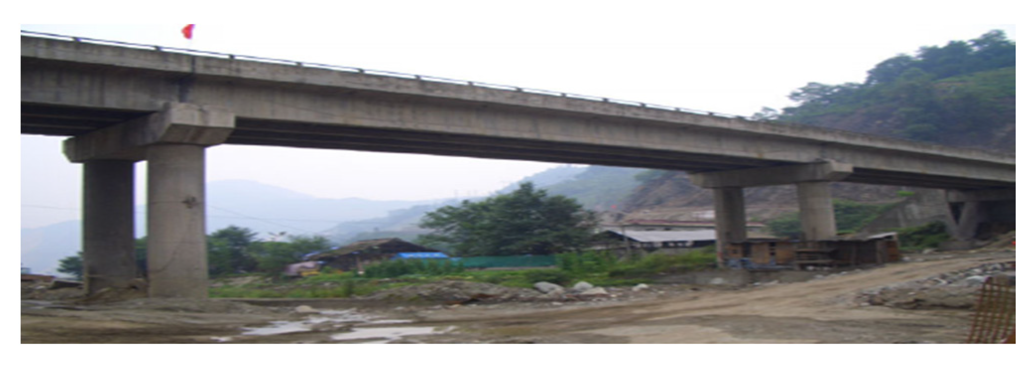
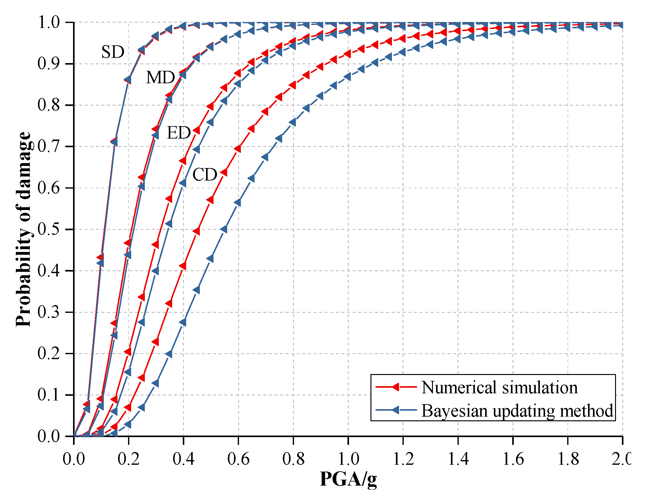
5.1. Correcting the Theoretical Seismic Vulnerability Curve of Simply Supported Bridge

Zheng et al. [40] used the probabilistic seismic demand analysis approach to establish an analytical seismic vulnerability model of typically simply supported girder bridge (Guxigou Middle Bridge, see Figure 2) in Wenchuan area. Based on survey data of damaged bridges from the Wenchuan earthquake, the uncertainty of the bridge structure parameters was evaluated. The Latin Hypercube Sampling method was used to sample the uncertainty parameters in the model to generate 160 typical bridge analysis samples in turn. Nonlinear dynamic transient analysis was preformed using the Wenchuan Earthquake ground motions and the seismic peak responses of key bridge components were recorded. By using the regression analysis method, a relationship between the ground motion intensity and seismic demand of key bridge components was established. Figure 3 shows the probabilistic seismic demand models [33,40]. After determining the limit state of the bridge components corresponding to four damage states (SD, MD, ED, and CD) of the bridge, the seismic vulnerability curves corresponding to the different damage states were generated based on the logarithmic normal distribution assumption. Based on adopting the reliability theory, the upper and lower bounds of the seismic vulnerability of the bridge system were calculated. Finally, the least squares regression was used to obtain the median value and log-standard deviation of the seismic vulnerability function of the bridge system, as shown in

Table 2. The seismic vulnerability curve parameters of Guxigou Middle Bridge.

Damage State	Numerical Simulation		Bayesian Updating Method
	$\mathbf{Median} \mathbf{Value} {\mathit{c}}_{\mathit{j}}$	$\mathbf{Log}\text{-}\mathbf{Standard} \mathbf{Deviation} {\mathit{\xi }}_{\mathit{j}}$	$\mathbf{Median} \mathbf{Value} {\mathit{c}}_{\mathit{j}}$	$\mathbf{Log}\text{-}\mathbf{Standard} \mathbf{Deviation} {\mathit{\xi }}_{\mathit{j}}$
SD	0.1099	0.4969	0.1116	0.5069
MD	0.2093	0.4635	0.2172	0.4711
ED	0.3156	0.5252	0.3436	0.5314
CD	0.4525	0.5535	0.5496	0.5343

[40]. Figure 4 shows the seismic vulnerability curve of the Guxigou Middle Bridge based on the simulation.

In this paper, the seismic vulnerability function parameters of Guxigou Middle Bridge obtained based on the numerical simulation were used as the prior information of Bayesian correction. Based on Bayesian method, the structural seismic demand information was calculated and corrected by combining the damage survey data during Wenchuan earthquake. Based on Bayesian parameter estimation method, the posterior probability of seismic demand information was obtained by Equations (7)–(9). Figure 5 shows the contrast diagram of the corrected seismic vulnerability curve of Guxigou Middle Bridge based on numerical simulation and seismic survey data. Table 2 shows two parameters of the numerical simulation method and Bayesian updating method.

It is found that the corrected seismic vulnerability curve is slightly lower than the seismic vulnerability curve of numerical simulation in Figure 5. The deviation of the corrected seismic vulnerability curve and the numerical simulation curve is caused by the uncertainty of the seismic wave. Therefore, the results of numerical simulation are safe to ensure the structural performance, safety, and stability under earthquakes. Figure 5 shows that the seismic reliability of the Guxigou Middle Bridge is higher when the earthquake intensity is lower, and its ability for maintaining the structural performance level is stronger. However, the seismic performance of this bridge is weaker when there are larger intensity earthquakes.

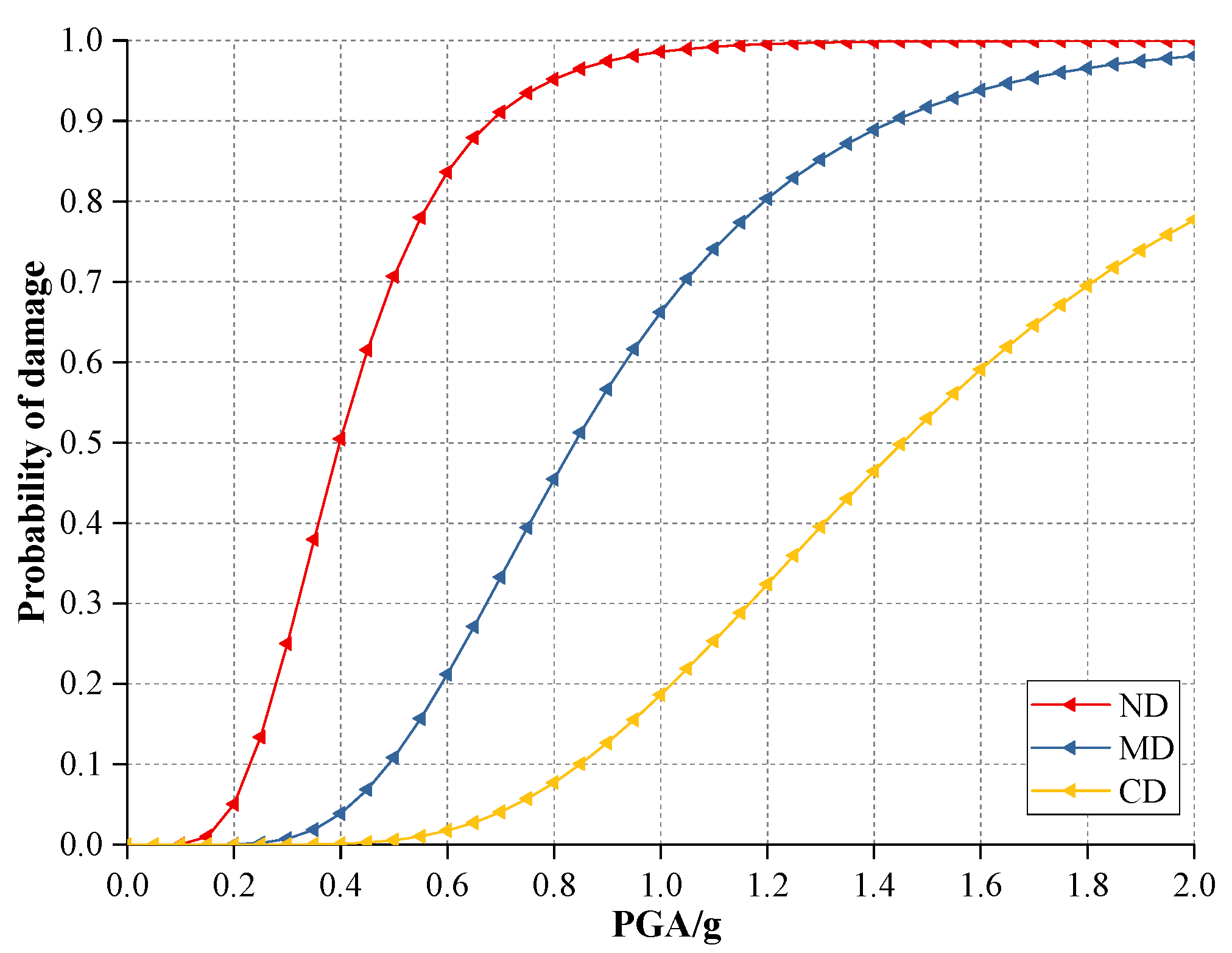
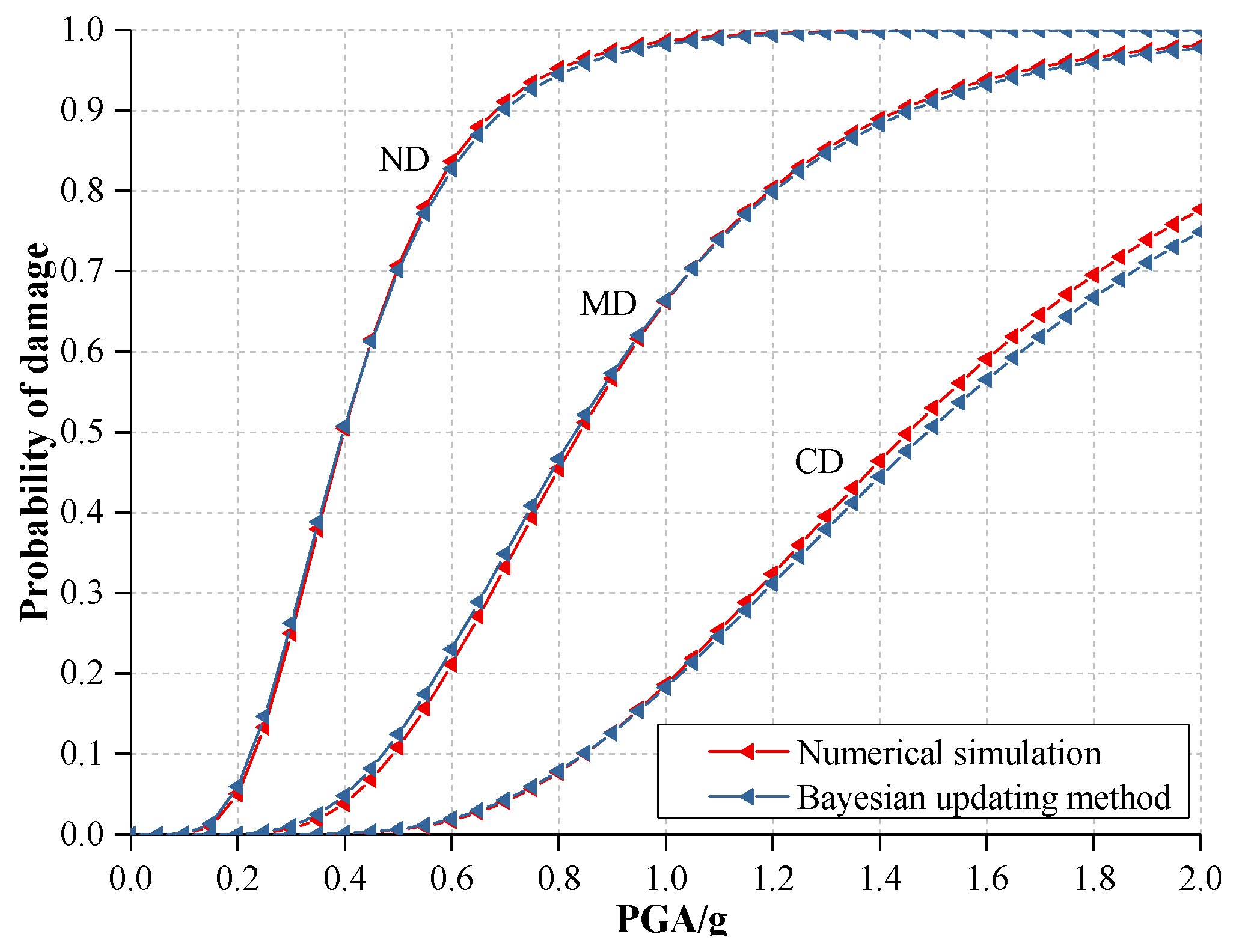
5.2. Correcting the Theoretical Seismic Vulnerability Curve of Continuous Girder Bridge

Wang et al. [41] selected a three-span pre-stressed reinforced concrete rigid frame bridge as the research object. The structural layout plan and elevation view are shown in Figure 6. Wang et al. used the structural nonlinear analysis software SAP2000 to analyze the dynamic characteristics and seismic response of the bridge and established a three-dimensional finite element model of the bridge. Based on the drift ratio of the bridge column, three limit states (ND, MD, and CD) of the bridge were taken as the limit states of the bridge, and the probability parameters of the three limit states were obtained. The incremental dynamic analysis method was used to calculate the probabilistic characteristics of the engineering demand parameters of the bridge at a given ground motion intensity. Based on the total probability theory, the probability was calculated when the bridge structure reached or exceeded the specified damage state at a given ground motion intensity. Finally, the seismic vulnerability curve of the bridge structure was obtained by fitting the discrete points.

Table 3. The seismic vulnerability curve parameters of three-span pre-stressed reinforced concrete rigid frame bridge.

Damage State	Numerical Simulation		Bayesian Updating Method
	$\mathbf{Median} \mathbf{Value} {\mathit{c}}_{\mathit{j}}$	$\mathbf{Log}\text{-}\mathbf{Standard} \mathbf{Deviation} {\mathit{\xi }}_{\mathit{j}}$	$\mathbf{Median} \mathbf{Value} {\mathit{c}}_{\mathit{j}}$	$\mathbf{Log}\text{-}\mathbf{Standard} \mathbf{Deviation} {\mathit{\xi }}_{\mathit{j}}$
ND	0.3980	0.2780	0.3965	0.2949
MD	0.8390	0.3810	0.8300	0.4013
CD	1.4530	0.4185	1.4884	0.4395

lists the median value and log-standard deviation of the seismic vulnerability function of the bridge system based on numerical simulation [41]. Figure 7 shows the vulnerability curve of the bridge based on the simulation.

In this paper, the seismic vulnerability function parameters (median value and log-standard deviation) of this bridge obtained based on the numerical simulation were used as the prior information of Bayesian correction. Based on the Bayesian parameter estimation method and combining survey damage data during the Wenchuan earthquake, the seismic demand information of the bridge structure was calculated according to Equations (7)–(9). The posterior probability of the post-earthquake demand of the bridge was obtained. Figure 8 shows a comparison of the seismic vulnerability curves of a three-span pre-stressed reinforced concrete continuous rigid frame bridge based on numerical simulation and seismic damage investigation data.

Figure 8 shows that the exceedance probability of the numerical simulation and the corrected seismic vulnerability curve based on seismic damage investigation data under the three working conditions is consistent and coincide with each other. Although there are some biases between the exceedance probability of the structural performance based on Bayesian updating method and the exceedance probability of the structural performance based on numerical simulation, the seismic performance of bridges is reliable, economical, and reasonable.

6. Post-Earthquake Traffic Capacity Assessment

As we all know, the transportation system in the earthquake area will suffer different degrees of damage after the earthquake. As an important part of the transportation system, the damaged degree and traffic capacity of the bridge system after the earthquake have a very important impact on the earthquake relief work. If the bridge structure is completely destroyed after the earthquake, its traffic is almost paralyzed, more air disaster relief forces must be considered. However, if the bridge structure is only slightly damaged after the earthquake, and ground transportation can still maintain a part of the operating state, then it may still be considered to rely mainly on the ground transportation system to complete the disaster relief transportation [24,42]. Therefore, it is of great significance to evaluate the post-earthquake state of bridges in the field of earthquake relief work.

In this paper, Guxigou Middle Bridge was taken as an example, which seismic vulnerability curve based on Bayesian updating method for each damage was used as the basis for assessing the traffic capacity after earthquake. Specifically, based on the corrected seismic vulnerability curves of the bridge, the percentages of various damage states under a certain ground motion were calculated by using the method provided in the reference [43]. Then, combining probabilistic results and expected values assigned for each damage level, the average damage level of the bridge under different ground motion intensity was calculated to obtain change of design traffic flow and variation curve of travel time under a certain traffic flow, which can provide a basis for the quick assessing of the traffic capacity of the bridge after an earthquake.

6.1. The Damage State Failure Probability of Guxigou Middle Bridge

Limit states (LS) describe the failure limit state of the structure, which is the limit of the adjacent damage state (DS), and the damage state is the interval between two adjacent limit states. Figure 9 shows the relationship between the limit state and damage state [34]. The limit state of Guxigou Middle Bridge structure was divided into four limit states, which includes SD (LS₁), MD (LS₂), ED (LS₃), and CD (LS₄). These four limit states divide the damage process of the bridge structure into five damaged states, which includes no damage (DS₁), slight damage (DS₁), moderate damage (DS₃), extensive damage (DS₄), and complete damage (DS₅) [34].

Suppose that $P_{f,L{S}_i}\left(x\right)$ represents the probability of exceeding the limit state LS_i of the bridge structure when the ground motion intensity is x, which is the value $F_{R_i}\left(x\right)$ of the seismic vulnerability function corresponding to LS_i at x. $P_{f,L{S}_i}\left(x\right)$ is called the limit state failure probability. Suppose that $P_{f,D{S}_i}\left(x\right)$ represents the probability when the bridge structure is in the damage state DS_i, which is the interval probability between the limit state LS_i-1 and the limit state LS_i of the bridge structure. $P_{f,D{S}_i}\left(x\right)$ is called the damage state failure probability. Taking LS₄ as an example, the limit state failure probability $P_{f,L{S}_3}\left(x\right)$ is equal to the sum of $P_{f,D{S}_4}\left(x\right)$ and $P_{f,D{S}_5}\left(x\right)$. The relationship between the limit state and the damage state can be expressed by Equation (10) [34].

$$F_{R_i}\left(x\right)=P_{f,L{S}_i}\left(x\right)={\displaystyle \sum }_{j=i+1}^5{P}_{f,D{S}_j}\left(x\right)$$

(10)

The seismic vulnerability curve (that is, the limit state failure probability curve) and correlations with the limit state and the damage state are shown in Figure 10.

According to the seismic vulnerability curves based on Bayesian updating method In Figure 5, the limit state failure probability of the bridge structure can be calculated by Equation (11).

Table 4. The damage state failure probability of Guxigou Middle Bridge under different peak ground accelerations (PGA).

PGA	${\mathit{P}}_{\mathit{f},\mathit{D}{\mathit{S}}_1}$	${\mathit{P}}_{\mathit{f},\mathit{D}{\mathit{S}}_2}$	${\mathit{P}}_{\mathit{f},\mathit{D}{\mathit{S}}_3}$	${\mathit{P}}_{\mathit{f},\mathit{D}{\mathit{S}}_4}$	${\mathit{P}}_{\mathit{f},\mathit{D}{\mathit{S}}_5}$
0.00	100.00%	0.00%	0.00%	0.00%	0.00%
0.05	93.35%	6.35%	0.28%	0.02%	0.00%
0.10	58.14%	34.53%	6.29%	0.97%	0.07%
0.15	29.00%	46.58%	18.38%	5.29%	0.75%
0.20	13.74%	42.39%	28.31%	12.63%	2.93%
0.25	6.56%	33.06%	32.80%	20.57%	7.02%
0.30	3.21%	24.07%	32.75%	27.12%	12.86%
0.35	1.62%	16.97%	30.03%	31.46%	19.92%
0.40	0.84%	11.81%	26.15%	33.59%	27.60%
0.45	0.45%	8.19%	22.04%	33.91%	35.41%
0.50	0.25%	5.68%	18.20%	32.89%	42.98%
0.55	0.14%	3.96%	14.83%	31.02%	50.05%
0.60	0.08%	2.78%	11.98%	28.64%	56.52%
0.65	0.05%	1.96%	9.63%	26.03%	62.33%
0.70	0.03%	1.40%	7.72%	23.39%	67.46%
0.75	0.02%	1.00%	6.18%	20.83%	71.97%
0.80	0.01%	0.72%	4.95%	18.43%	75.89%
0.85	0.01%	0.53%	3.97%	16.22%	79.28%
0.90	0.00%	0.39%	3.19%	14.22%	82.20%
0.95	0.00%	0.28%	2.56%	12.44%	84.72%
1.00	0.00%	0.21%	2.07%	10.85%	86.87%
1.05	0.00%	0.16%	1.67%	9.46%	88.72%
1.10	0.00%	0.12%	1.35%	8.23%	90.30%
1.15	0.00%	0.09%	1.10%	7.16%	91.65%
1.20	0.00%	0.07%	0.89%	6.23%	92.81%
1.25	0.00%	0.05%	0.73%	5.42%	93.80%
1.30	0.00%	0.04%	0.60%	4.72%	94.65%
1.35	0.00%	0.03%	0.49%	4.11%	95.37%
1.40	0.00%	0.02%	0.40%	3.58%	95.99%
1.45	0.00%	0.02%	0.33%	3.12%	96.53%
1.50	0.00%	0.01%	0.28%	2.72%	96.99%
1.55	0.00%	0.01%	0.23%	2.38%	97.38%
1.60	0.00%	0.01%	0.19%	2.08%	97.73%
1.65	0.00%	0.01%	0.16%	1.82%	98.02%
1.70	0.00%	0.01%	0.13%	1.59%	98.27%
1.75	0.00%	0.00%	0.11%	1.39%	98.49%
1.80	0.00%	0.00%	0.09%	1.22%	98.68%
1.85	0.00%	0.00%	0.08%	1.07%	98.85%
1.90	0.00%	0.00%	0.07%	0.94%	98.99%
1.95	0.00%	0.00%	0.06%	0.83%	99.11%
2.00	0.00%	0.00%	0.05%	0.73%	99.22%

gives the damage state failure probability of Guxigou Middle Bridge under different peak ground accelerations PGA. Figure 11 shows the failure probability curves of five damage states.

$$P_{f,D{S}_i}\left(x\right)=\{\begin{array}{c}1-F_{R_i}\left(x\right) \left(i=1\right)\\ F_{R_{i-1}}\left(x\right)-F_{R_i}\left(x\right) \left(i=2,3,4\right)\\ F_{R_4}\left(x\right) \left(i=5\right)\end{array}$$

(11)

6.2. Design Traffic Flow Assessment

Based on existing research [43,44], the upper bound of the corrected seismic vulnerability curves of Guxigou Middle Bridge corresponding to each damage state were taken as the basis for calculating traffic flow. According to the references [42,43], the probabilistic results and expected values ($\mathrm{the} \mathrm{values} \in \left[0,4\right], \mathrm{where},0 \mathrm{is} \mathrm{no} \mathrm{damage} \mathrm{state} \mathrm{and} 4 \mathrm{is} \mathrm{complete} \mathrm{damage} \mathrm{state}$) assigned for each damage level were combined to obtain the average damage level value $l_b$ of Guxigou Middle Bridge under different ground motion intensity, which can be calculated by Equation (12).

$$l_b=0\ast P_{f,D{S}_1}+1\ast P_{f,D{S}_2}+2\ast P_{f,D{S}_3}+3\ast P_{f,D{S}_4}+4\ast P_{f,D{S}_5}$$

(12)

In this paper, the design speed ${\mathrm{v}}^c$ of Guxigou Middle Bridge was 100 km/h, the number of lanes $b$ was 3, and the minimum distance ${\mathrm{s}}_{\min }$ between the two vehicles at the design speed was 100 m. The designed critical flow $f^{\mathrm{co}}$ was the critical value of traffic flow at the beginning of congested road conditions (that is the actual traffic capacity). According to Equation (13), the designed critical flow was 3000 vehicles/hour.

$$f^{co}=\frac{{\mathrm{v}}^c}{s_{min}}·b$$

(13)

The change of traffic flow $f^c$ with the increase of PGA under the ground motion intensity can be calculated according to Equation (14) [43].

Table 5. Design traffic flow changes with PGA.

PGA	lb	fc	PGA	lb	fc	PGA	lb	fc	PGA	lb	fc
0	3.743	3000	0.55	3.955	98	1.05	3.989	4	1.55	0.000	2
0.05	3.782	3000	0.6	3.962	58	1.1	3.991	3	1.6	0.000	2
0.1	3.816	2994	0.65	3.967	36	1.15	3.992	3	1.65	0.000	2
0.15	3.844	2903	0.7	3.971	23	1.2	0.000	3	1.7	0.000	2
0.2	3.868	2592	0.75	3.976	16	1.25	0.000	2	1.75	0.000	2
0.25	3.887	2055	0.8	3.979	11	1.3	0.000	2	1.8	0.000	2
0.3	3.904	1441	0.85	3.981	8	1.35	0.000	2	1.85	0.000	2
0.35	3.918	910	0.9	3.984	6	1.4	0.000	2	1.9	0.000	2
0.4	3.930	536	0.95	3.986	5	1.45	0.000	2	1.95	0.000	1
0.45	3.940	303	1	3.988	4	1.5	0.000	2	2	0.000	1
0.5	3.948	171

shows the change of traffic flow $f^{\mathrm{c}}$ changing with the peak ground acceleration PGA.

$$f^c=f^{co}·\exp \left[-a^{RC}·{\left(l_b\right)}^{{\beta }^{RC}}\right]$$

(14)

where, $l_b$ represents the average damage level of the bridge under different seismic intensities, $a^{RC}$ and ${\beta }^{RC}$ are related parameters, which generally take 0.03 and 4, respectively.

The change of traffic flow with the increase of the ground motion intensity were calculated according to Equation (14). Figure 12 shows that the normal performance of the bridge structure declines little, and the traffic flow does not change significantly when the earthquake acceleration is less than 0.10 g (that is, the earthquake intensity is small). When the seismic acceleration is more than 0.10 g, Guxigou Middle Bridge is greatly damaged and the bearing capacity of the bridge structure reduces with the increase of the ground motion intensity. Moreover, the main function and the traffic flow of the bridge rapidly decrease. When the earthquake acceleration reaches 0.30 g, the traffic flow reduces to 1441 vehicles/hour. As a result, the traffic flow of Guxigou Middle Bridge should be strictly controlled at this time, which provides a basis for the decision-makers to exercise the rescue and transportation after the earthquake.

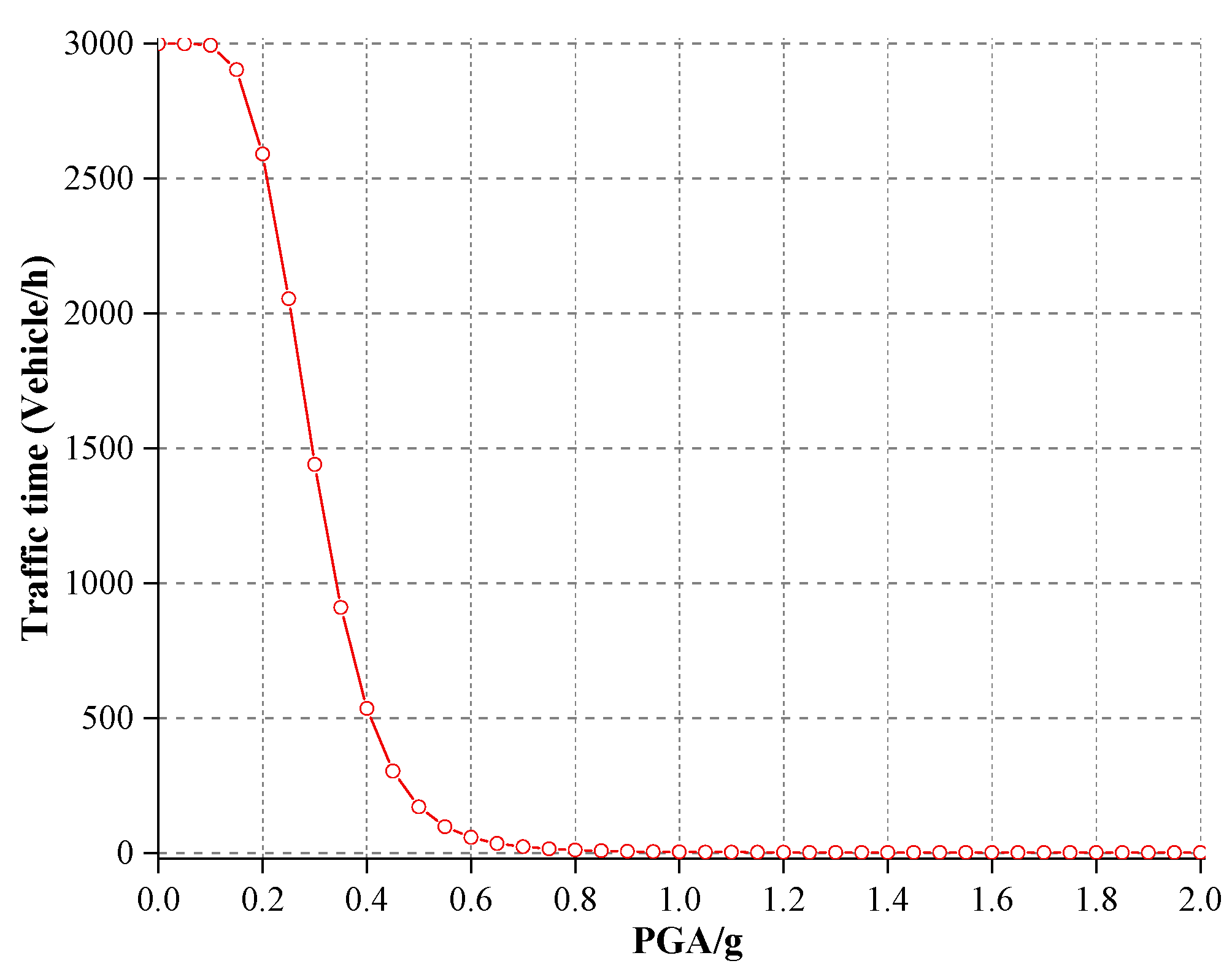
6.3. Traffic Time Assessment

Traffic impedance refers to the relationship between road travel time and traffic load, intersection delay, and intersection load. Under earthquake action, the actual traffic capacity of each section reduces to a certain extent because the damage degree of each section is different. Therefore, the time required for the vehicles to pass through the bridges is also changed. Based on the calculation of the designed traffic flow, the time required for the vehicle to cross Guxigou Middle Bridge was calculated according to Equation (15) [42,43].

$$c=c^0{[1+{\alpha }^{CF}(\frac{f}{f^{c0}})]}^{{\beta }^{CF}}$$

(15)

where, $c^0=L/{\mathrm{v}}^c$ is the time required for the vehicle to pass through the bridge during free flow. In the traffic flow distribution procedure of the US Highway Bureau, ${\alpha }^{CF}$ and ${\beta }^{CF}$ are the blocking factors, which take 0.15 and 4, respectively. The impedance c on the section/bridge is the traffic time when the traffic flow is $f$.

As the research object of this paper, the size of the main bridge of Guxigou Middle Bridge is 3 m × 30 m. The time required for the vehicle to pass through the bridge under earthquake action is shown in Figure 13.

Figure 13 shows that there is no fluctuation in the time of opening when the traffic flow is below the critical flow (that is the percentage of traffic flow is less than 100%). While the flow traffic exceeds the critical traffic flow, traffic time curve is increased with the increase in traffic flow. Road congestion situation intensifies, which affects the normal passage of vehicles. When the bridge is damaged during earthquakes, the structure is damaged, affecting the normal service performance and the normal traffic, the passing time of vehicle is increased. According to Equation (15), the traffic time changes with the earthquake acceleration under certain traffic flow is calculated, and the result is shown in Figure 14.

Figure 14 shows the traffic time is almost unchanged when the peak acceleration of earthquake is below 0.20 g. At the same time, it does not affect the normal service performance of the bridge. When the peak acceleration of earthquake increases from 0.20 g to 0.30 g, the traffic time changes significantly, and the bridge structure is greatly damaged, and the normal passage of vehicles is blocked. When the rescue is needed after the earthquake, the traffic diversion control should be considered to avoid causing congestion in the prime time for rescue. When the peak acceleration of earthquake is greater than 0.30 g, the traffic time is of rapid growth. At this time, the bridge structure suffered severe damage or even lost its normal using performance and the carrying capacity could not operate normally. Therefore, the earthquake relief should consider changing the rescue route or using air traffic force to avoid this traffic node.

7. Conclusion

(1)

This study used Bayesian correction method to update the seismic vulnerability curves of bridges under several damage states. In the case that the experimental conditions are not sufficient for statistical probability analysis, this method makes full use of the existing historical earthquake damage experience and numerical simulation results to determine the probability distribution parameters of the bridge structure. The results show that the corrected seismic vulnerability curves are closer to the actual situation, which provides a new idea for the reliability analysis of bridge structure.

(2)

Based on the corrected seismic vulnerability curves of Guxigou Middle Bridge, the traffic flow and traffic time of the bridge after earthquakes were quickly evaluated. The results show that the traffic flow decreases and the traffic time increases when the peak acceleration of earthquake increases. This method has certain practicability and scientificity, which is of great significance for evaluating the sustainable traffic capacity of bridges after earthquakes.

References

1. Jiang, Z.Z.; Li, Y.Y.; Sun, Q.F.; Fan, Y. Research on Theoretical Model of Traffic Capacity of Highway Bridges after Earthquake. J. Disaster Prev. Mitig. Eng. 2015, 35, 226–231. [Google Scholar]
2. Transportation Research Road; Highway Capacity Manual (HCM), National Research Council: Washington, DC, USA, 2001.
3. Cabboi, A.; Magalhaes, F.; Gentile, C.; Cunha, A. Automated modal identification and tracking: Application to an iron arch bridge. Struct. Control Health Monit. 2017, 24. [Google Scholar] [CrossRef]
4. Chalouhi, E.K.; Gonzalez, I.; Gentile, C.; Karoumi, R. Damage detection in railway bridges using Machine Learning: Application to a historic structure. In 10th International Conference on Structural Dynamics (EURODYN); Sapienza Univ Rome, Fac Civil & Ind Engn: Rome, Italy, 2017. [Google Scholar] [CrossRef]
5. Intergovernmental Panel on Climate Change (IPCC). Determinants of Risk: Exposure and Vulnerability, Managing the Risks of Extreme Events and Disasters to Advance Climate Change Adaptation (SREX); Cambridge University Press (CUP): New York, NY, USA, 2012. [Google Scholar]
6. Barbat, A.H.; Carreno, M.L.; Pujades, L.G.; Lantada, N.; Cardona, O.D.; Marulanda, M.C. Seismic vulnerability and risk evaluation methods for urban areas. A review with application to a pilot area. Struct. Infrastruct. Eng. 2010, 6, 17–38. [Google Scholar] [CrossRef]
7. Chieffo, N.; Clementi, F.; Formisano, A.; Lenci, S. Comparative fragility methods for seismic assessment of masonry buildings located in Muccia (Italy). J. Build. Eng. 2019, 25. [Google Scholar] [CrossRef]
8. Pan, Y.; Agrawal, A.K.; Ghosn, M. Seismic fragility of continuous steel highway bridges in New York State. J. Bridge Eng. 2007, 12, 689–699. [Google Scholar] [CrossRef]
9. Lourenco, P.B.; Roque, J.A. Simplified indexes for the seismic vulnerability of ancient masonry buildings. Constr. Build. Mater. 2006, 20, 200–208. [Google Scholar] [CrossRef] [Green Version]
10. Karim, K.R.; Yamazaki, F. Effect of earthquake ground motions on fragility curves of highway bridge piers based on numerical simulation. Earthq. Eng. Struct. Dyn. 2001, 30, 1839–1856. [Google Scholar] [CrossRef]
11. Stefanidou, S.P.; Kappos, A.J. Bridge-specific fragility analysis: When is it really necessary? Bull. Earthq. Eng. 2019, 17, 2245–2280. [Google Scholar] [CrossRef] [Green Version]
12. Zourgui, N.H.; Kibboua, A.; Taki, M. Using full bridge model to develop analytical fragility curves for typical concrete bridge piers. Gradevinar 2018, 70, 519–530. [Google Scholar] [CrossRef] [Green Version]
13. Zampieri, P.; Zanini, M.A.; Faleschini, F. Derivation of analytical seismic fragility functions for common masonry bridge types: Methodology and application to real cases. Eng. Fail. Anal. 2016, 68, 275–291. [Google Scholar] [CrossRef]
14. Li, H.N.; Cheng, H.; Wang, D.S. A Review of advances in seismic fragility research on bridge structures. Eng. Mech. 2018, 35, 1–16. [Google Scholar]
15. Kiremidjian, A.A.; Basoz, N. Evaluation of bridge damage data from recent earthquake. Nceer Bull. 1997, 11, 1–27. [Google Scholar]
16. Laura, M.; Francesco, C.; Antonio, F. Static and dynamic testing of highway bridges: A best practice example. J. Civ. Struct. Health Monit. 2020, 10, 43–56. [Google Scholar] [CrossRef]
17. Zani, G.L.; Martinelli, P.; Galli, A.; Gentile, C.; di Prisco, M. Seismic Assessment of a 14th-Century Stone Arch Bridge: Role of Soil-Structure Interaction. J. Bridge Eng. 2019, 24. [Google Scholar] [CrossRef]
18. Cornell, C.A.; Jalayer, F.; Hamburger, R.O.; Foutch, D.A. Probabilistic basis for 2000 SAC federal emergency management agency steel moment frame guidelines. J. Struct. Eng. 2002, 128, 526–533. [Google Scholar] [CrossRef] [Green Version]
19. California Department of Transportation (Caltrans). The Northridge Earthquake; Caltrans PEQIT Report; Div of Structures: Sacramento, CA, USA, 1994. [Google Scholar]
20. Shinozuka, M.; Feng, M.Q.; Lee, J.; Naganuma, T. Statistical analysis of fragility curves. J. Eng. Mech. Asce 2000, 126, 1224–1231. [Google Scholar] [CrossRef] [Green Version]
21. Hwang, H.; Liu, J.B. Seismic fragility analysis of reinforced concrete bridges. China Civ. Eng. J. 2004, 37, 47–51. [Google Scholar]
22. Choi, E.S.; DesRoches, R.; Nielson, B. Seismic fragility of typical bridges in moderate seismic zones. Eng. Struct. 2004, 26, 187–199. [Google Scholar] [CrossRef]
23. Duan, M.Z.; Ya, H.Y.; Li, S.S.; Cao, H.Y. Assessment Model for Traffic Capaity after Seismic Disaster. J. Chongqing Jiaotong Univ. (Nat. Sci.) 2017, 36, 79–85. [Google Scholar]
24. Lan, R.Q.; Feng, B.; Wang, Z.F. Study on the fast assessment of traffic capacity of highway bridges after strong earthquakes. World Earthq. Eng. 2009, 25, 81–87. [Google Scholar]
25. Liu, Z.L. Seismic Performance Assessment of Urban Bridge Network Considering the Post-Disaster Evacuation Capacity. Master’s Thesis, Harbin Institute of Technology, Harbin, China, 2015. [Google Scholar]
26. Wu, W.P.; Li, L.F.; Hu, S.C.; Xu, Z.J. Research review and future prospect of the seismic fragility analysis for the highway bridges. J. Earthq. Eng. Eng. Vib. 2017, 37, 85–96. [Google Scholar]
27. Cornell, C.A. Engineering seismic risk analysis. Bull. Seismol. Soc. Am. 1968, 58, 1583–1606. [Google Scholar]
28. Shinozuka, M.; Kim, S.H.; Kushiyama, S.; Yi, J.H. Fragility curves of concrete bridges retrofitted by column jacketing. Earthq. Eng. Eng. Vib. 2002, 1, 195–205. [Google Scholar] [CrossRef]
29. Shinozuka, M.; Murachi, Y.; Dong, X.J.; Zhou, Y.W.; Orlikowski, M.J. Effect of seismic retrofit of bridges on transportation networks. Earthq. Eng. Eng. Vib. 2003, 2, 169–179. [Google Scholar] [CrossRef] [Green Version]
30. Ghosh, J.; Padgett, J.E. Aging Considerations in the Development of Time-Dependent Seismic Fragility Curves. J. Struct. Eng. 2010, 136, 1497–1511. [Google Scholar] [CrossRef]
31. Karim, K.R.; Yamazaki, F. A simplified method of constructing fragility curves for highway bridges. Earthq. Eng. Struct. Dyn. 2003, 32, 1603–1626. [Google Scholar] [CrossRef]
32. Wu, Z.Y.; Jia, Z.P.; Liu, X.X. Calibration of Analytical Fragility Curves Based on Empirical Data of Bridges. Appl. Math. Mech. 2014, 35, 723–736. [Google Scholar]
33. Chen, L.B. Seismic Vulnerability Analysis for Highway Bridges in Wenchuan Region. Ph.D. Thesis, Southwest Jiaotong University, Chengdu, China, 2007. [Google Scholar]
34. Lv, D.G.; Yu, X.H. Theoretical study of probabilistic seismic risk assessment based on analytical functions of seismic fragility. J. Build. Struct. 2013, 34, 41–48. [Google Scholar]
35. Ang, A.H.-S.; Tang, W.H. Probability Concepts in Engineering Planning and design; John Wiley and Sons Inc.: New York, NY, USA, 1984. [Google Scholar]
36. Zhang, G.W.; Liu, L.Y. A generalized Bayes method for determining the probability distribution parameters of random variables. Chin. J. Geotech. Eng. 1995, 17, 91–94. [Google Scholar]
37. Xu, C.; Yang, L.D. Test of Goodness of Fit of Random Variables and Baysian Estimation of Distribution Parameters. J. Tongji Univ. 1998, 26, 340–344. [Google Scholar]
38. Ma, J.R.; Xu, J. Discussion on Fuzzy Bayes Method for Parameter Estimation. J. Chengdu Univ. (Nat. Sci. Ed.) 2011, 30, 223–225. [Google Scholar]
39. Lin, Q.L. A Study on Seismic Fragility of Highway Bridges Based on Wenchuan Earthquake Damage. Ph.D. Thesis, Institute of Engineering Mechanics, China Earthquake Administration, Harbin, China, 2017. [Google Scholar]
40. Zheng, K.F.; Chen, L.B.; Zhuang, W.L.; Ma, H.S.; Zhang, J.J. Bridge Vulnerability Analysis Based on Probability Seismic Demand Models. Eng. Mech. 2013, 30, 165–172. [Google Scholar]
41. Wang, J.M.; Wang, G.L.; Nie, J.G.; Zhao, L.H. Probability based seismic risk analysis of bridge structures. China Civ. Eng. J. 2010, 43, 86–93. [Google Scholar]
42. Gao, N. Seismic Vulnerability Analysis of Long-Span Continous Beam Bridge. Master’s Thesis, Southwest Jiaotong University, Chengdu, China, 2017. [Google Scholar]
43. Bocchini, P.; Frangopol, D.M. A stochastic computational framework for the joint transportation network fragility analysis and traffic flow distribution under extreme events. Probab. Eng. Mech. 2011, 26, 182–193. [Google Scholar] [CrossRef]
44. Comell, C.A. Bounds on the reliability of structural systems. J. Struct. Div. 1967, 93, 171–200. [Google Scholar]
Figure 1. The seismic vulnerability curve of bridges based on historical damage data.
Sustainability 12 01898 g001
Figure 2. The Guxigou Middle Bridge.
Sustainability 12 01898 g002
Figure 3. Probabilistic seismic demand models.
Sustainability 12 01898 g003
Figure 4. The seismic vulnerability curves of Guxigou Middle Bridge based on numerical simulation.
Sustainability 12 01898 g004
Figure 5. Comparison of the seismic vulnerability curves of Guxigou Middle Bridge based on numerical simulation and Bayesian updating method.
Sustainability 12 01898 g005
Figure 6. Plan and elevation of three-span pre-stressed reinforced concrete rigid frame bridge (unit: cm).
Sustainability 12 01898 g006
Figure 7. The seismic vulnerability curves of three-span pre-stressed reinforced concrete rigid frame bridge based on numerical simulation.
Sustainability 12 01898 g007
Figure 8. Comparison of the seismic vulnerability curves of three-span pre-stressed reinforced concrete continuous rigid frame bridge based on numerical simulation and Bayesian updating.
Sustainability 12 01898 g008
Figure 9. Limit state and the damage state.
Sustainability 12 01898 g009
Figure 10. Sketch map of seismic vulnerability curves and correlations with limit states and damage states.
Sustainability 12 01898 g010
Figure 11. Sketch map of failure probability curves of damage states.
Sustainability 12 01898 g011
Figure 12. Variation curve of the design traffic flow changing with PGA.
Sustainability 12 01898 g012
Figure 13. Variation curve of the traffic time changing with traffic flow.
Sustainability 12 01898 g013
Figure 14. Variation curve of the traffic time changing with PGA.
Sustainability 12 01898 g014