1. Introduction
Carbon emissions control is an environmental issue of widespread international concern. The longitudinal slope design indicator has crucial effect on the carbon emitted by various vehicles. When driving conditions such as speed, vehicle type, vehicle load, road pavement conditions, and road environment remain unchanged, vehicles consume fluctuating quantities of fuel when moving uphill versus as they perform additional work to overcome height differences on uphill roads [
1,
2]. The relationship between longitudinal slope design indicators and vehicle carbon emissions has a great deal of practical significance and has been explored by many researchers. Researchers have found that targeting longitudinal slope roads may be an effective approach to reducing fuel consumption and carbon emissions [
2,
3]. Quantifying the carbon emissions of vehicles in vertical profile and exploring the influence of design indicators on carbon emissions are important for the design of low-carbon vertical profiles. Governments and road operation management agencies may be able to directly control the total carbon emissions of two-way traffic flows on highways constituted by integral subgrades. The influence of design indexes on the carbon emissions of vehicles traversing flat, uphill, and downhill road sections must first be determined to support such control measures. Previous studies have also shown that energy-saving and emission-reduction effects can be achieved by controlling longitudinal slope design indexes in particular [
1,
2,
3].
Fuel economy refers to the ability of a vehicle to operate economically, i.e., consuming as little fuel as possible, while ensuring dynamic performance [
4,
5]. Fuel consumption in this case corresponds to minimum carbon emissions levels [
3]. Certain scholars dedicated to this subject have focused on improving energy efficiency and reducing greenhouse gas emissions in transportation systems through research on new energy vehicle [
6,
7] and controlling vehicle speeds [
8,
9,
10]. Dreier et al. [
6] analyzed the influence of passenger load, driving cycle, fuel price and four different types of buses on the cost of transport service on a rapid transit route in Curitiba, Brazil. The technology–economic optimization model was used to identify an alternative to the conventional bi-articulated bus fleet currently in operation, with the goal of minimizing weekly transportation service costs. Dreier et al. [
7] also conducted a well-to-wheel comparative analysis of fossil energy use and greenhouse gas emissions for conventional, hybrid-electric and plug-in hybrid-electric city buses in the Curitiba bus rapid transit system; they found that advanced powertrains and larger passenger capacity utilization can contribute to the system’s sustainability. According to numerous previous studies [
8,
9,
10], a vehicle consumes less fuel when traveling at a constant speed than at a fluctuating speed. Chang and Morlok [
9] suggested that the optimal speed profile for fuel consumption of a motor vehicle, under various roadway characteristics, is achieved at cruising speed.
The design indexes of the longitudinal slope affect the driving power of individual vehicles [
3]. Vehicle power, in turn, is closely related to fuel consumption and carbon emissions [
2,
3]. Various micro carbon emission models, including the Comprehensive Modal Emissions Model (CMEM) [
11,
12,
13] and Motor Vehicle Emission Simulator (MOVES) [
14] reflect the real-time operating conditions of vehicles. Barth and Scora et al. [
11,
12] conducted laboratory dynamometer tests on 343 light-duty trucks to test vehicle speed, fuel consumption, and exhaust emissions data under various operating conditions. The regression estimation method was adopted to construct the CMEM [
12,
13] of a light truck with factors such as road gradient, instantaneous speed, engine transmission coefficient, vehicle frontal area, and road friction coefficient. This study was limited by the fact that the laboratory dynamometer test does not fully reflect real-world driving conditions. There are also differences in vehicle performance and fuel characteristics in various regions which limit the practical application of the CMEM [
13,
15,
16].
The US Environmental Protection Agency adopted the Portable Emission Measurement System (PEMS) to collect vehicle speed and exhaust emissions data. Vehicle specific power and instantaneous speed were then used to characterize actual vehicle operating conditions. The Motor Vehicle Exhaust Emission Model (MOVES) [
14] was developed based on measured vehicle operating conditions, road type, gradient, temperature, fuel consumption, and exhaust emissions data. Ko et al. [
17] used a dynamics non-uniform velocity model established by Lan and Menendez [
18] to simulate the instantaneous speed of a 120 kg/kW truck on a longitudinal slope, then used MOVES to predict the carbon emissions of the truck as it traveled uphill. The gradient was shown to have the greatest impact on the truck’s carbon emissions among all indicators observed. When the mileage was 3000 m, the carbon emissions of the vehicle on the 9% gradient were about four-fold greater than on a straight, flat road. However, the influence of driving behavior, such as acceleration and deceleration, was not ruled out—thus, no substantive suggestions regarding the gradient value in the low-carbon design of the longitudinal slope have been put forward to data. Moreover, the default values of related parameters in the model apply to local US conditions, which differ from vehicle performance, fuel characteristics, temperature, altitude, and other notable test factors in China [
13,
15,
16]. This model cannot be directly applied to estimate the fuel consumption and carbon emissions of Chinese vehicles.
Vehicle fuel consumption models based on vehicle dynamics theory are relatively authoritative. Scholars have investigated the fuel consumption and driving power of vehicles under certain driving forces using vehicle dynamics theory [
8,
9,
10], including a few studies on the influence of highway longitudinal gradients on fuel consumption. Barth and Scora et al. [
11,
12] analyzed the driving power of a vehicle on uphill sections with factors such as engine transmission coefficient, instantaneous speed, road gradient, vehicle frontal area, and road friction coefficient using vehicle dynamics theory; they found a close relationship between driving force and fuel consumption. Different driving forces interact with different operating conditions. The CMEM models of light-duty trucks was developed based on measured operating conditions data from laboratory dynamometer tests. Kang [
8] used the tractive effort model of a vehicle on the longitudinal slope road proposed by Chang [
9] to build a new model of the relationship between fuel consumption and tractive effort with fuel consumption rate as a conversion factor. Fuel consumption rate is affected by factors such as vehicle load, engine type, and environmental conditions. Fuel consumed is approximately proportional to total propulsive work performed by the prime movers. Chang [
9] indicated that vehicle dynamic conditions on flat road, uphill road, and downhill road sections notably differ, and divided the vehicle dynamic load on the downhill section into two cases: one where the gravity potential energy completely offsets the air resistance and the rolling resistance, and one where the gravity potential energy is greater than the road resistance. Various balance gradients applicable to the first case have been proposed for different vehicle loads, but mechanical resistance has not yet been considered and only the fuel consumption in the first case was assessed. The fuel consumption rate in the models was also idealized and was considered a constant. There has been no model verification based on field test data [
8,
9]. It is worth noting that the models indicate that vehicle fuel consumption is approximately proportional to the total propulsive work of the vehicle, and that the slope affects the total driving power to a certain extent.
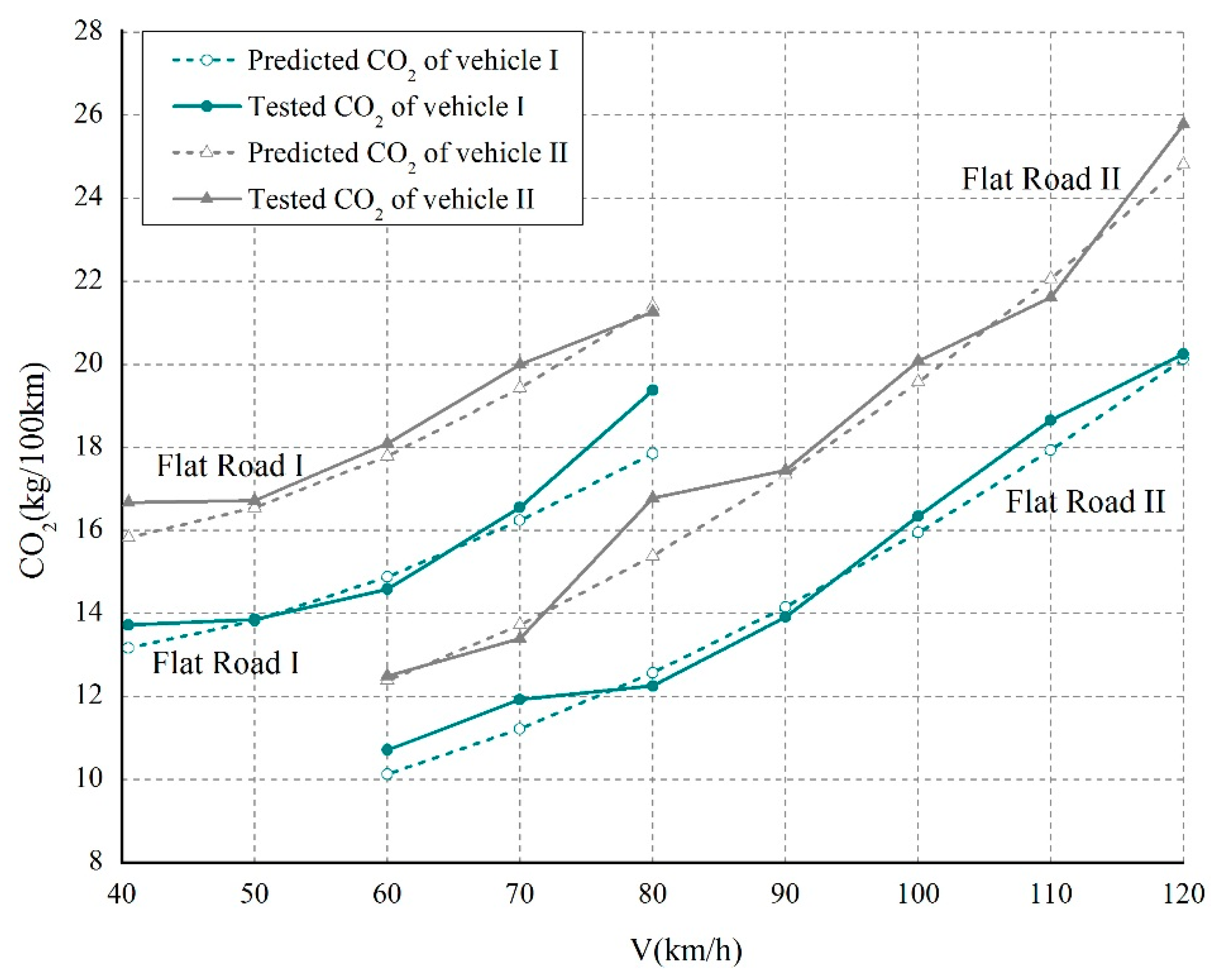
Kanok and Barth [
1] conducted a fuel consumption field test on uphill, downhill, and flat road sections with a maximum gradient of 6% in a passenger car maintaining a cruise speed of 96 km/h. The results showed that the vehicle’s fuel consumption was greatest on the uphill section, followed by the flat road and finally the downhill section. The fuel economy on a plain route was also found to be better than on a mountainous route. The relationship between the fuel consumption measured and the road grade appeared to be linear within the grade range –2% to 2%, which implies that there would be no difference in fuel consumption among round-trip mountainous routes within such a range versus flat route. The fuel consumption of the vehicle on the flat road was 18% lower than the fuel consumption on the combination of uphill and downhill roads with a gradient of 6%. Due to lack of theoretical basis and insufficient experimental data for each road grade, this study did not reveal the extent to which the gradient affects vehicle fuel consumption. The gradient was not clearly defined when the fuel consumption was similar on the uphill-downhill combination and flat road. The extant research on vehicle fuel consumption and carbon emissions centers on driving behavior [
11,
12,
13,
14,
17] and vehicle power loads [
8,
9,
10]. The road gradient is known to more significantly influence vehicle carbon emission rate than the factors of rolling resistance, acceleration rate, frontal area, temperature [
10]. Existing micro carbon emission models, such as CEME and MOVES, were established on large quantities of measured or simulated data [
11,
12,
13,
14]; arguably, the theoretical basis of these models is insufficient. The default parameters in these micro models are also inconsistent with China’s specific conditions [
15,
16] and cannot be directly applied to the estimation of vehicle fuel consumption or carbon emissions in China. Scholars have yet to clarify the impact of gradient on vehicle fuel consumption. It is also not yet empirically known whether vehicle fuel consumption is equivalent on flat roads versus uphill-downhill combination roads. Considering that traffic is usually two-way, it is necessary to explore this issue. It is impossible to secure the scientific mathematical models and theoretical guidance necessary for decision-making regarding innovative, low-carbon highway longitudinal slope designs without this information. The mathematical fuel consumption models established using vehicle dynamics theory are relatively authoritative, but they do not consider the mechanical resistance and fuel consumption rates of different fuel types [
8,
9]. It is worth considering that the research on vehicle fuel consumption and driving power under certain driving force conditions based on vehicle dynamics theory [
8,
9,
10] does provide a theoretical basis for establishing a mathematical model of propulsive energy, fuel consumption, and carbon emissions for vehicles on longitudinal slopes in China. Passenger cars have good power performance and can generally travel uphill at the average speed of all vehicles on the road [
19,
20]. The fuel consumption of a motor vehicle is approximately minimized by operating at cruising speed [
8,
9,
10]. In this study, the speed of a passenger car on the longitudinal slope road was assumed to be uniform in conformity with real-world vehicle operation conditions, and as is conducive to further research on the energy-saving and low-carbon highway longitudinal slope design.
The present study was conducted to establish a quantified model of carbon emissions of passenger cars on uphill, downhill, and flat roads. The carbon emissions rules of passenger cars on longitudinal slope sections were investigated to secure low-carbon and fuel-economy-related longitudinal slope design indicators. The energy conversion of a vehicle in overcoming height differences was determined based on vehicle longitudinal dynamics theory, the law of conservation of mechanical energy, and the first law of thermodynamics. Universally applicable fuel consumption and carbon emission models for passenger cars on highway longitudinal slopes were established to explore the corresponding carbon emission rules. A theoretical model was evaluated using field test data. A combination of theoretical and empirical research methods was deployed to ensure reliable conclusions.
The remainder of this paper is organized as follows.
Section 2 discusses the law of conservation of mechanical energy and the first law of thermodynamics as-utilized to assess the energy conversion of a vehicle on a longitudinal slope road. The conversion of energy, fuel consumption, and carbon emissions proposed by the Intergovernmental Panel on Climate Change (IPCC) is used to account for the carbon emissions of the passenger car as it traverses a longitudinal slope. The importance of the balance gradient is highlighted in this section as well. In
Section 3, the accuracy of the passenger car’s carbon emission model is evaluated by field tests conducted on flat, uphill, downhill, symmetrical slope combination, and continuous longitudinal slop road sections. The carbon emission rule of vehicles on the longitudinal highway slope is confirmed by test results.
Section 4 summarizes the key findings alongside a discussion on the limitations of this work.
2. Carbon Emission Model
In this section, the law of conservation of mechanical energy, the first law of thermodynamics, the vehicle longitudinal dynamics theory, and the accounting method proposed by IPCC for energy, fuel consumption, and carbon emissions are used to establish the carbon emission model of passenger car on uphill, downhill, and flat sections. Meanwhile, the proposed carbon emission model reveals the carbon emission rules of vehicles on the longitudinal section.
For the proposed energy conversion, fuel consumption, and carbon emission models, the following are assumed:
a. The driver of the passenger car maintains a uniform speed. The American Association of State Highway and Transportation Officials (AASHTO) indicates that the passenger car is relatively unaffected by the road gradient when driving on a longitudinal slope due to its acceptable power performance. Almost all passenger cars can traverse 4% to 5% steep slopes at a uniform speed without deceleration [
19]. The Japan Road Association states that the general gradient value ensures that passenger cars can travel uphill at a uniform speed; this speed is the average speed of all vehicles on the road [
20]. The Chinese “Technical Standard of Highway Engineering” indicates that passenger vehicles generally run at a constant and relatively high speed on highways in a free flow pattern, do not interfere with each other, and do not significantly fluctuate in speed [
21]. The assumption that the passenger vehicle maintains a uniform speed in traversing a longitudinal slope is consistent with real-world driving conditions in free flow patterns. Cruising can prevent the interference from speed fluctuations on carbon emissions, which is conducive to research on fuel economy and carbon reduction in highway longitudinal slope design;
b. All frictional heat is absorbed by the brake drum when braking. The effects of other parts of the brake chamber during heat generation and heat dissipation are generally negligible [
4,
22], which is conducive to the establishment of an energy conversion model for vehicles on longitudinal slope sections. The positive work of gravity converts the gravitational potential energy into the kinetic energy of the vehicle, during grade descent. The kinetic energy is controlled by the brake operation, while the friction at the drum interface simultaneously generates heat [
22].
2.1. Energy Conversion Model
As the vehicle runs, chemical energy in its fuel is converted into mechanical energy through a combustion process in the engine. Mechanical energy is converted into kinetic energy via the vehicle’s transmission and tire systems. There is energy loss in every link, mainly in regards to engine combustion efficiency, transmission system efficiency, tire rolling resistance, aerodynamic resistance, and brake friction [
4,
5,
23]. The vehicle dynamic conditions on a flat road, uphill road, and downhill road sections are different [
3,
4,
5]. Vehicle dynamics theory was used in this study to analyze the force of vehicles on various road sections and to establish vehicle energy conversion models accordingly. The influence of the gradient on vehicle carbon emissions was observed by comparing the vehicle energy conversion model of the flat road and a combination of symmetrical slope road sections.
2.1.1. Flat Road
Aerodynamic resistance and rolling resistance act on the vehicle as the vehicle travels across a flat, straight road. The effective tractive effort of the vehicle is related to its engine power, travel speed, and transmission efficiency [
4,
5,
24], as follows:
where F
i is the indicated tractive effort (N), which is equal to the total resistance of the vehicle [
4,
5]; F is the effective tractive effort. The transmission efficiency n
tf is reflected in the mechanical losses of the various transmission system components (transmission, transmission shaft, differential, and drive shaft). As the vehicle travels at a uniform speed, the engine speed is in an optimal working state and the transmission efficiency remains constant. When predicting vehicle power performance, the transmission efficiency of the current common passenger car is usually estimated to be approximately 85% [
4,
24].
The vehicle is also subject to aerodynamic resistance during driving. The aerodynamic resistance is proportional to the dynamic pressure of the relative speed of the air [
5,
25], as follows:
where A is the vehicle frontal area (m
2), i.e., the area of the car from the front to the rear [
5].
ρ is the air density, generally 1.2258N·s
2/m
4. The aerodynamic resistance coefficient C
D is related to the shape of the vehicle. The air resistance coefficients of various shapes of vehicles can be obtained from related documents on vehicle characteristics [
5,
25]. V is the relative speed of the vehicle and air considering the angle between the wind and the driving direction (m/s).
On the highway longitudinal slope, the gradient is very small. It can be assumed that the length of the slope is approximately equal to the horizontal distance. The work done by aerodynamic resistance is as follows:
Rolling resistance is related to tire type, road type, and speed [
22,
24]. It can be approximated as follows:
where v is the vehicle speed (km/h). The rolling coefficient C
r is related to the pavement type and condition, typical values are available in the literature of Rakha [
24]. Rolling resistance constants C
2 and C
3 are related to tire type and can be assigned values as determined empirically. For the mixed tires commonly used in passenger cars, C
2 = 5.3 and C
3 = 0.044 [
22].
The work done by rolling resistance is:
2.1.2. Uphill
The tractive effort of vehicles is affected by driving resistance on uphill roads. The driving resistance includes slope resistance, rolling resistance, and aerodynamic resistance. The slope resistance is the component of the vehicle’s weight parallel to the road surface [
4]. The vehicle’s gravity performs negative work parallel to the road surface, as indicated in Equations (6) and (7).
where i is the road gradient (%).
2.1.3. Downhill
A portion of the gravity parallel to the road surface plays a positive role as the vehicle travels downhill. Rolling resistance, aerodynamic resistance, and braking force do negative work. It is worth noting that when the vehicle travels uphill along a straight trajectory, the torque direction of the engine is transmitted from the engine to the wheels. When the vehicle goes downhill, conversely, gravity increases the kinetic energy of the vehicle. If the accelerator pedal is not pressed and the gear is still in the gear position, the engine is in the reversed state and the torque direction is opposing. The reverse tractive force of the transmission system generates resistance to the vehicle [
4,
5]. A greater gradient produces greater gravitational potential energy. When the gradient is large, the vehicle will accelerate even if the accelerator is not pressed and the vehicle can slide downhill in the gear position. A portion of the gravitational potential energy offsets the energy lost by the transmission system [
4]. Chang [
9] analyzed a case in which the vehicle requires no braking to maintain a constant speed on the downgrade. The inherent forces (rolling resistance, wind resistance) and gradient force cancel one another in this case and no propulsive work is required. However, the transmission resistance was not considered.
There are three cases of driving behavior which emerge as the vehicle maintains a cruise speed across various gradients.
a. In Case I, when the accelerator is not pressed, the vehicle can slide downhill in the gear position at a cruise speed. The gravitational potential energy can offset the negative worked by rolling resistance, wind resistance, and reverse tractive force [
4,
5,
9]. In this case, the vehicle meets the following energy relationship:
where, W
t’ is the indicated the energy loss caused by reverse tractive force (J).
When the vehicle does not slide downhill at the gear position, the reverse traction does not work and W
t’ = 0 [
4]. The balance gradient corresponding to the cruise speed can be calculated according to the specific driving road conditions of the vehicle.
b. In Case II, when the work of driving resistance and aerodynamic resistance is greater than the gravitational potential energy, the driver must step on the accelerator to provide additional energy and ensure that the vehicle maintains the cruise speed. The energy relationship is as follows:
c. In Case III, when the work of driving resistance and aerodynamic resistance is less than the gravitational potential energy, the remaining gravitational potential energy is converted into kinetic energy which provides a certain increase in the vehicle’s speed. In order to maintain the cruise speed at this point, the driver needs to step on the brake to ensure that the kinetic energy not increased. The braking force produces brake drum heat Q
h [
22]. According to the first law of thermodynamics, the energy relationship in this case is as follows:
The energy loss value on the downhill road is theoretically equal to the difference between the energy of gravity potential and the energy consumed by driving resistance. Compared to the propulsive energy traveling uphill with the balance gradient, the increase in propulsive energy when traveling uphill (which overcomes the increased elevation difference) is equal to the energy loss of vehicle when traveling downhill.
2.1.4. Symmetrical Slope Combination Road
The energy of a combination of symmetrical uphill-downhill and flat roads were compared to explore the impact of the road gradient on vehicle carbon emissions The uphill-downhill combination is required to be symmetrical in gradient and slope length, and the slope length is equal to the flat road length. The energy provided by the effective tractive effort of the vehicle on the flat, uphill, and downhill road sections in this case are W1, W2, W3, respectively. The propulsive energy formulations of the vehicle on flat and uphill sections are expressed as follows:
The vehicle’s energy conversion formulations on downhill road sections in Case I, Case II, Case III are reflected in Equations (13) and (14), Equation (15), Equations (16) and (17), respectively.
The respective energy relationships of the vehicle on the three types of symmetrical slope combination roads are as follows.
Equations (11) and (19) show that the vehicle carbon emissions of the longitudinal slope combination road II and the flat road are equivalent. The difference between energy consumed by the transmission system and energy loss caused by reverse tractive force was usually ignored in derivation of vehicle longitudinal power [
4]. This indicates that the carbon emissions of the symmetrical slope combination road I and the flat road are basically equivalent. The energy provided by the engine on symmetrical slope combination roads I, II and the flat road is basically equal. The difference in fuel consumption between the uphill section and flat road is equal to the difference in fuel consumption between the flat road and downhill section, as shown in Equations (11), (18) and (19).
In the symmetrical slope combination road III, the gradient is greater than the balance gradient. The energy loss during braking on the downhill section is equal to the difference in energy provided by the tractive effort between the uphill section and the flat road, as shown in Equations (11) and (20).
When the gradient of the longitudinal slope is not greater than the balance gradient, the vehicle emits roughly the same amount of carbon on the symmetrical slope combination road and the flat road. When the gradient of the downhill slope exceeds the balance gradient, a steeper gradient and longer grade length cause more energy to be lost by the brake. The energy loss is equal to the propulsive energy difference on the uphill and a flat road with equal mileage. Brake energy loss is offset by the excess propulsive energy on the uphill compared with the propulsive energy on the flat road with equal mileage of symmetrical slope combination roads. It is not conducive to energy-saving or emission-reduction in regard to the two-way traffic on the longitudinal slope. The balance gradient is the minimum gradient that affects vehicle’s fuel consumption and carbon emissions of two-way traffic. The gradient should be avoided to be greater than the balance gradient during the low-carbon longitudinal slope design.
2.1.5. Continuous Longitudinal Slope
The energy of continuous longitudinal slope sections and single longitudinal slope sections were compared to explore the carbon emissions rules of passenger vehicles on the vertical profile. The propulsive energy corresponding to the continuous uphill road section can be calculated by Equations (21) and (22). The energy is equal to the propulsive energy on the slope with average gradient and equal mileage, as reflected in Equation (23).
When the gradient of each downhill section on the continuous downhill road is not greater than the balance gradient, the propulsive energy can be calculated by Equations (24) and (25). The energy is equal to the propulsive energy on the slope with the average gradient and equal mileage as derived by Equation (26):
where i
j, x
j represent the gradient and length of each slope section, respectively. The number of single slope sections on the continuous longitudinal slope is n;
is the average gradient (%) of the continuous longitudinal slope.
A quadratic parabola is usually used as a vertical curve to connect the two longitudinal slopes at the turning point of the slope sections (Equation (27)) [
26]. It is necessary to consider the vertical curve section in predicting the vehicle’s carbon emissions on longitudinal slopes.
where x is the lateral distance, that is, the distance from any point to the starting point of the vertical curve;
is the gradient of any point of the vertical curve,
. At the beginning of the vertical curve, x = 0,
. At the end of the vertical curve, x=L,
. i
1 and i
2 are the gradients of the longitudinal slopes connected to the ends of the vertical curve. L is the length of the vertical curve.
The vertical curve is divided into n longitudinal slopes each with length of Δx. The fuel consumption of the vehicle in the vertical curve section is the sum of the fuel consumption of the vehicle on the longitudinal slope of different gradients corresponding to each step, as shown in Equation (28).
The vertical curve section can be regarded as the connection of multiple slope sections. The energy of vehicles on the vertical curve satisfies the above energy conversion relationship.
For continuous longitudinal slopes with a fixed height differences, when the gradient of each downhill section is not greater than the balance gradient, the propulsion energy on the continuous longitudinal segment is equal to the propulsive energy on the slope with average gradient and equal mileage regardless of the design index (gradient and slope length) of each slope section.
2.2. Conversion Among Energy, Fuel Consumption, Carbon Emissions
Fuel is the source of propulsive energy for vehicles. In recent years, China’s motor vehicles have been required to meet the National Fifth-phase Motor Vehicle Pollutant Emission standards [
27]. Gasoline vehicles are generally equipped with a spark ignition gasoline engine. Moreover, the characteristic of fuels supplied to gasoline vehicles must meet the National Fifth-phase Standards of Gasoline for Motor Vehicles [
28]. The density of gasoline(p) type 92#, 95#, and 98# is 0.725 kg/L, 0.737 kg/L, and 0.753 kg/L, respectively [
29]. The average low calorific value of gasoline(A) is 44.800 (kJ/kg). The calorific values of burning one liter of different density gasoline is 32480 kJ/L, 33017.6 kJ/L, and 33734.4 kJ/L respectively. According to the first law of thermodynamics, energy is conserved when thermal energy and mechanical energy are converted. The fuel utilization rate is the proportion of fuel that provides drive energy to the total fuel, as presented in Equation (29). The fuel utilization rate of a spark ignition gasoline engine, n
m, is generally 27% [
5,
10,
30]. The remaining energy is converted into heat and then lost. The fuel consumption of gasoline of different densities in China can be calculated according to Equations (30)–(32).
where, Fuel indicates fuel consumption (L).
The IPCC accounting method [
31] was adopted here to observe the relationship between vehicle fuel consumption and carbon emissions, as shown in Equation (33). This prevented measurement error otherwise caused by various factors when directly detecting gas from the exhaust pipe of the test vehicle. The conclusions of this study are comparable with extant results from similar work in other countries; the universal applicability of the research results presented here is guaranteed [
15,
16]. Data relevant to the extant vehicle fuel characteristics in China can be found in the “National Communication on Climate Change of China” [
32,
33]. The potential carbon emission factor (C) is 18.9 (t/TJ), the carbon conversion factor(K) is 44/12, and the carbon oxidation rate (B) is 98%. It can be obtained that the carbon emission from burning one liter of gasoline type 92#, 95#, and 98# is 2.206 kg/L, 2.242 kg/L, and 2.291 kg/L, respectively, as shown in Equations (34)–(36).
where, CO
2 represents carbon emissions (kg).
The vehicle engine burns a certain amount of fuel to provide the effective tractive effort to overcome aerodynamic resistance and rolling resistance while traversing a flat road [
5,
22]. The effective tractive effort of the vehicle on the uphill section must overcome slope resistance, aerodynamic resistance, and rolling resistance [
4,
5]. Greater tractive effort results in greater the fuel consumption and more carbon emissions [
3]. On the downhill section, when the vehicle’s gravitational potential energy is equal to or greater than the energy consumed by aerodynamic resistance and rolling resistance, the vehicle does not need to provide any additional tractive effort and there is no fuel consumed or carbon emitted. When the aerodynamic resistance and rolling resistance consumes more energy than the gravitational potential energy, the vehicle must provide tractive effort to maintain the cruise speed and consumes a certain amount of fuel while emitting a certain amount of carbon [
4,
5,
9]. There is constant idle fuel when the vehicle is not under neutral operation conditions [
3].
Considering the heat generation of different fuel types, transmission efficiency and fuel utilization rate, the fuel consumption of different fuel types can be determined as the engine provides a certain driving energy, as indicated in Equations (37)–(39). When fuels of different densities produce equal driving energy, they correspond to uniform quantities of carbon emissions, as demonstrated in Equations (40)–(42).
where, Q is the constant idle fuel rate (L/h). t is the travel time (h).


