Abstract
The emission of pollutants from vehicles is presented as a prime factor deteriorating air quality. Thus, seeking public policies encouraging the use and the development of more sustainable vehicles is paramount to preserve populations’ health. To better understand the health risks caused by air pollution and exclusively by mobile sources urges the question of which input variables should be considered. Therefore, this research aims to estimate the impacts on populations’ health related to road transport variables for São Paulo, Brazil, the largest metropolis in South America. We used three Artificial Neural Networks (ANN) (Multilayer Perceptron—MLP, Extreme Learning Machines—ELM, and Echo State Neural Networks—ESN) to estimate the impacts of carbon monoxide, nitrogen oxides, ozone, sulfur dioxide, and particulate matter on outcomes for respiratory diseases (morbidity—hospital admissions and mortality). We also used unusual inputs, such as road vehicles fleet, distributed and sold fuels amount, and vehicle average mileage. We also used deseasonalization and the Variable Selection Methods (VSM) (Mutual Information Filter and Wrapper). The results showed that the VSM excluded some variables, but the best performances were reached considering all of them. The ELM achieved the best overall results to morbidity, and the ESN to mortality, both using deseasonalization. Our study makes an important contribution to the following United Nations Sustainable Development Goals: 3—good health and well-being, 7—affordable and clean energy, and 11—sustainable cities and communities. These research findings will guide government about future legislations, public policies aiming to warranty and improve the health system.
1. Introduction
According to the Lancet Commission on pollution and health [1], 9 million premature deaths were attributable to air pollution in 2015 (16% of all deaths in the world), greater than deaths by AIDS, tuberculosis and malaria combined, and around 15 times those from all wars and other kinds of violence.
Due to the high impact of air pollutants on human health, it is considered a big issue faced by developed and developing countries [2,3], and mobile sources are a well-known villain at urban centers [4,5,6]. Therefore, the International Agency for Research on Cancer (IARC) classified diesel engine exhaust emissions as carcinogenic, increasing government responsibility to establish legislations aiming at the diminution of vehicle emissions [4,5,6]. In this context, the Brazilian government created, in 1986, a program to control air pollution by vehicles (PROCONVE) aiming to progressively reduce air pollutants emissions from vehicles. For example, from 2009 to 2013, the country reduced 42% of nitrogen oxides (NOx) light duty vehicles emissions. Additionally, the government launched the “Route 2030 Program—Mobility and Logistic” with one major aim of improving vehicles’ sustainability by enhancing the production of electric vehicles and those using biofuels, which may reduce air pollutants emission [7].
Many researches aiming to investigate urban air pollution were done in the past few years. More precisely, Andrade et al. [8] showed the evolution of transport emissions of the last 30 years and future perspectives for São Paulo, Brazil. The authors concluded that the transportation sector is a big challenge to urban areas, being responsible for most of the air pollutants emission, and highlighted that the use of cleaner fuels and new engine technologies is paramount for improving air quality. The WHO [9] reported one of the main sources of urban ambient particulate matter (PM) is vehicle emissions, and estimated a relative share of 34% at Brazilian urban sites. Andrade et al. [10] and Miranda et al. [11] performed source distribution analyses in six Brazilian state capitals, including the Metropolitan Region of São Paulo. The authors concluded that the largest percentage of pollutant concentrations is due to high traffic volumes.
Bell et al. [12] assessed the relation between energetic policies and pollutants concentrations in three Latin American cities: Mexico City (Mexico), Santiago (Chile), and São Paulo (Brazil). For each city, a hypothetic emission scenario was developed to estimate how the actual and future patterns of fossil fuel use can affect the air quality. Health effect analyses were done to estimate the number of morbidity and mortality events that could be avoided if modest air pollution control policies were adopted. The authors found health expenses of roughly $21 to $165 billion (US) could be avoided.
Although pollution challenges have been faced by a variety of Brazilian cities, the São Paulo megacity deserves attention, as it is considered the major urban conglomerate of South America [13], one of the 31 global megacities [14], and its intensive growth is worsening the air quality of São Paulo, according to Andrade et al. [8], mainly due to mobile sources.
To better understand the influence of air pollution from mobile sources on the population’s health raises the question as to which input variables should be considered. Usually, researchers consider only climatic variables as inputs to assess health effects linked to air pollution [15,16,17,18,19,20]. However, other input variables should be considered to take into account the contribution of mobile sources, such as road transport ones, as new engine technologies and alternative fuels are arising and electric vehicles production is also being encouraged [8,21,22].
Patra et al. [23] presented a review of researches about particulate matter impact on human health, pointing out empiric evidences between the following parameters: humidity; silt content and moisture content of particulate matter; vehicle speed; drop height; vehicle weight; size of loader; exposed surface area; loading and unloading frequency; number of dry days; and others.
Road transport variables, such as vehicles fleet, used fuels, and others are available monthly; thus regression models commonly used to estimate air pollution impacts on population health may not capture relationships between variables, due to small databases. As an alternative, Artificial Neural Networks (ANN) were preferred. These methodologies are important candidates to solve mapping problems, since they are capable of approximating any nonlinear functions if they are limited, continuous, differentiable and defined in a compact space [24]. The ANN are characterized by an intrinsic learning capability and a present generalization ability [24,25,26].
In air the pollution field, Artificial Neural Networks have been widely used for air pollutants forecasting [27,28,29,30,31,32]. For example, in 1998, Gardner and Dorling [33] already concluded that ANN is a successful methodology to predict air pollutants concentration and that it provides better results than linear statistical methods due to the non-linear behavior of data.
Nagendra and Khare [34] used ANN to explain traffic effects on the concentration of PM10. Zolghadri and Cazaurand [35] also predicted PM10 concentrations using ANN, and concluded that inclusion of traffic emissions data improved the results. Fernando et al. [36] predicted PM10 concentrations at metropolitan areas, showing that ANN are easier, faster and more economic without compromising prediction precision. Additionally, Cabaneros et al. [30] reported a review of researches with a focus on air pollution forecasting using ANN from 2001 to February 2019, resulting in 139 peer-reviewed articles.
However, ANN have been used less to estimate the human health impacts of air pollution. Wang et al. [37] studied the impact of nitrogen oxides (NOx), sulfur dioxide (SO2), carbon monoxide (CO), total suspended particles (TSP), and PM10 on mortality for respiratory diseases in Beijing (China) using ANN. Kassomenos et al. [16] predicted the daily number of hospital admissions for cardio respiratory diseases due to CO, NO2, SO2, ozone (O3), black smoke concentrations, and meteorological data (temperature, relative humidity, and wind speed and direction) in Athens, Greece. The authors applied Generalized Linear Models (GLM) and ANN, showing the superior performance of the last. Fontes et al. [38] developed ANN to predict the impact of traffic emissions on human health, using as input traffic and meteorological data. Sundaram et al. [39] applied ANN to predict respiratory, cardiovascular and total mortality due to temperature, relative humidity, and CO, SO2, NOx, hydrocarbons, O3, and particulates concentrations. Tadano et al. [40] assessed PM10, temperature and relative humidity impact on hospital admissions for respiratory diseases in Campinas city, Brazil. Polezer et al. [20] showed that ANN can be applied to forecast air pollution impact on human health, even when the dataset is short or has many gaps (a Brazilian data reality). Araujo et al. [41] used ten distinct ANN, four ensembles and Generalized Linear Models (GLM) to estimate PM10 impact on hospital admissions for respiratory diseases in Campinas and São Paulo cities, Brazil, concluding that ANN and ensembles had better performances than GLM.
Subsequently, to estimate health effects related to road transport variables, we considered monthly input data from 2003 to 2017 for: road vehicles fleet; distributed and sold vehicles by fuels (gasoline, ethanol, diesel, and hybrid/electric); vehicle average mileage; concentration of gases (carbon monoxide—CO, nitrogen oxides—NOx, ozone—O3, and sulfur dioxide—SO2); and particulate matter less than 10 m in aerodynamic diameter (PM10); as output, we considered morbidity and mortality from respiratory diseases (International Classification of Diseases ICD-10/J00-J99). As mentioned, São Paulo was the target of our research.
To do so, we used the Variable Selection Methods and Mutual Information Filter and Wrapper together with three Artificial Neural Network (ANN) architectures: Multilayer Perceptron (MLP), Extreme Learning Machines (ELM), and Echo State Networks (ESN).
This research will provide useful information to the development of new technologies, aiming more consistent public policies to improve population life quality, such as air quality, health, and sustainable urban mobility.
2. Methods Theory
2.1. Deseasonalization and Stationarization
Many real-time series present seasonal behaviors, mainly due to variations in the weather during a time window [42]. For example, the temperature changes according to the season, being higher in the summer and lower in the winter, and the rainfall periods are different in each season depending on the location [25,42].
The aforementioned cases show that the seasonal pattern is present in the real world and that it may disturb the prediction capability of the models. In this sense, the application of a mathematical preprocessing technique named deseasonalization prior to the effective data insertion in the models and the prediction can be useful [26].
Siqueira et al. [26] presented a procedure to deseasonalize monthly seasonal streamflow series. This method produces a new series with zero mean and unit variance, which is approximately stationary, and is given by Equation (1):
where Si,m are the samples of the original series which is transformed into a new series Zi,m; and are the mean and the standard deviations of each month m, respectively, estimated using Equations (2) and (3):
where i = 1, 2,…, Ny are the corresponding year for the month m = 1, 2,…,12.
In addition to the deseasonalization application, data stationarization is a good way to transform a series into a stationary one, even if it does not have a seasonal component [43,44]. In this case, the mean and standard deviation are calculated to the whole series, using Equations (4) and (5):
where N is the total number of samples available.
Then, the new stationary series is given by Equation (6) [42]:
It is important to mention that the seasonal component is reinserted after predictions and before the calculation of performance metrics.
2.2. Input Selection
Variable selection is an approach aiming to identify the best set of inputs that increase the approximation capability of a predictor. This process is very important, as it can reduce the number of parameters to be adjusted by the model, which leads to computational effort reduction and helps understand the data [45]. We used Mutual Information and Wrappers as variable selection techniques.
2.2.1. Mutual Information
The Mutual Information (MI) method is a type of filter approach to subset selection. Filters are characterized by data-based methods, as the subset is chosen according to some correlation between the input candidate and the target [45,46].
The MI comes from the information theory and measures the nonlinear dependence between inputs [26,47]. The mutual information among two independent variables (x and y) is given by Equation (7):
where fx(xi) and fy(yi) are the respective marginal distributions of xi and yi, fxy(xi,yi) is the joint probability density function, and (xi, yi) are the respective i-th pair of samples, with i=1, 2,…, N.
The aforementioned variables calculation in Equation (7) is given by city-block kernel functions, because they do not assume some distribution a priori. In addition, the bootstrap method is used to determine the confidence level [43].
2.2.2. Wrappers
The wrapper methodology for subset selection is quite different from the filters as it depends on the predictor [45]. Considering N, the total number of inputs, subsets are created, and the predictor adjustment and validation to each subset are done; we then observe the achieved performances. Therefore, the selected subset is the one that leads to the best results.
The wrapper’s main advantage is that the model is taken into account to analyze the influence of each input. However, to be model-dependent, its computational effort tends to be elevated, as the model has to be adjusted to each candidate subset [46].
In this sense, forward selection is often used to reduce the number of adjusted models. To do so, initially an empty subset of inputs is considered. Then the model is adjusted considering each single input variable and the one that leads to the best performance is selected to the final subset. After that, the model is trained considering two inputs, the one selected in the previous step and the remaining (N–1) variables. The second variable selected is the one that leads to the smallest error, along with the first. These steps are repeated until the size of the subset is N, which means all of the variables are in it. The subset that leads to the best error metrics is chosen [26].
2.3. Artificial Neural Networks
This research used three architectures of Artificial Neural Networks (ANN): Multilayer Perceptron (MLP), Extreme Learning Machines (ELM), and Echo State Networks (ESN), to estimate road traffic variables’ impact on human health. Due to the similarities in their structure, the ELM and ESN are collectively known as Unorganized Machines (UMs) [25].
2.3.1. Multilayer Perceptron
The Multilayer Perceptron (MLP) is the most known and used Artificial Neural Network (ANN) worldwide. It is a universal approximator, since it is capable of approximating any nonlinear, continuous, limited, and differentiable function [24]. The MLP is composed of groups of artificial neurons called layers: the first layer is responsible for transmitting the input signal to the hidden layers; these produce a nonlinear mapping, transforming the input signal to another space; and the last one is the output layer, which receives the transformed signal and, by means of linear combinations, generates the network output [24]. In the MLP architecture, the same layer neurons are not connected and do not exchange information, while neurons of disjoint layers are connected. This is a characteristic of feedforward networks, which do not have recurrence or feedback loops [48].
The information processing of an MLP can be expressed as follows. Initially, consider u as the vector containing the network inputs, b as the polarization vector (bias), and as the weights of the intermediate layer, with n = 1,..., N being the index of each input, k = 1,..., K indicating the neuron, and the connections of the output neuron. Therefore, the output of the network is given by Equation (8):
where f is the activation function of the hidden neurons and fs is a linear activation function of the output neurons.
The training process of a neural network consists of adjusting the synaptic weights of the artificial neurons [24]. In the MLP, an iterative process is applied, usually by means of an unrestricted linear optimization algorithm solution [49]. To do so, the error gradient between the output network and the desired response is calculated using the backpropagation algorithm. The steepest descent is the algorithm most often applied to reduce this error [24].
It is noted that the user has to define the stop criterion. Often, the maximum number of iterations is adopted. It is important to mention that the cross-validation method must be applied to define the most appropriate topology and to avoid overfitting [49].
2.3.2. Extreme Learning Machines
Extreme Learning Machines (ELM) are single layer feedforward neural networks, introduced by Huang et al. [50]. In this proposal, the neurons’ arrangement is quite similar to the traditional MLP architecture. However, ELM present a remarkable dissemblance in the training process [48].
The proposers proved that randomly generated weights of the hidden layer can stand untuned. The only previous condition is that the activation function of the intermediate neurons needs to be continuously differentiable [48]. Additionally, they demonstrated that ELM are universal approximators, as the insertion of new neurons in the intermediate layer leads to a decrease in the output error [26]. The training process of an ELM becomes simple and solely involves finding the best set of neuron weights in the output layer. This problem can be performed by solving a linear regression problem. Huang et al. [48] suggest the use of the Moore–Penrose generalized inverse operation to overcome the task, as this technique simultaneously minimizes the norm of the output weight vector and the mean square error between the network output and the desired signal.
In this work, considering the set of inputs , with n = 1,…, N being the corresponding input data, the activation of the neurons in the intermediate layer (the output of this layer) is given by Equation (9):
where is the matrix containing the hidden layer weights, b is a column vector of bias and fh(.) specifies neuron activation functions.
The network output signal y is generated according to Equation (10):
where Wout is the output layer weights.
Finally, the training process, as mentioned, is performed by the application of the Moore–Penrose inverse operation, according to Equation (11):
where Xh is the matrix containing the hidden layer outputs, is the pseudo-inverse matrix, and d is the vector with the desired outputs (target).
2.3.3. Echo State Networks
Echo State Networks (ESN) were proposed by Jaeger [51]. They present similarities with ELM in terms of their simplicity in the training process. The main difference is that ESN are Recurrent Neural Networks (RNN), presenting feedback loops of information, with some outputs reinserted as inputs [52].
Jaeger [51] proved that, under specific conditions, the W matrix representing the dynamic reservoir is a nonlinear transformation directly influenced by the recent history of the input signal (hence the term echo). It allows the intermediate layer to be set in advance and can be kept unchanged during the training. Therefore, only the output layer has to be adjusted by means of least squares problem solution. The author named this condition “echo state propriety” [52].
ESN present recurrent connections within the intermediate layer, called the dynamic reservoir. The neurons activation in the reservoir (the output of this layer) is influenced by the current input and the previous state, according to Equation (12):
where is the input signal, Win is the input layer, W is the reservoir that presents the synaptic weights of the feedback connections and fh(.) = [f1(.), f2(.), …, fN(.)] are the activation functions.
The ESN output signal is calculated by Equation (13):
Jaeger [51] suggests a way to generate the reservoir that respects the echo state propriety. In this proposal, he created a W sparse matrix according to Equation (14). The elements (synaptic weights) of this matrix are given by:
Finally, as in ELM, the training process is performed applying the Moore–Penrose inverse operation, as in Equation (15):
where is the matrix containing the reservoir outputs and d is the desired response.
3. Case Study
The goal of this study is to forecast mortality and morbidity for respiratory diseases, considering variables regarding road vehicles transport, in São Paulo city, Brazil. The input variables are categorized as: road vehicles fleet; distributed and sold fuels amount (gasoline, ethanol, diesel, and hybrid/electric); vehicle average mileage; gases (CO, NOx, O3, and SO2); and PM10 concentrations. The considered outputs were morbidity and mortality for respiratory diseases. Monthly data for a long period (from January 2003 to December 2017) were used instead of a shorter daily series due to lack of daily information about road transport variables, such as vehicles fleet and fuel distribution.
São Paulo is the most populous city in South America and the seventh most populous city on Earth; it has approximately 12,038,175 inhabitants in a 1521 km2 area and has 8,036,824 motor vehicles circulating every day. It is also an economic hub of Latin America and has a Human Development Index (HDI) of 0.805. The city presents air pollutants concentration around twice the Air Quality Guidelines established by the World Health Organization [9,53,54].
The temporal series of motor vehicles number in São Paulo city were obtained from the statistical series of the National Department of Transit [53]. The National Agency of Petroleum, Natural Gas and Biofuels [55] provided the distribution of fuels for retailers (gasoline, ethanol, diesel, and hybrid/electric). The vehicle average mileage, PM10, NOx, O3, SO2 [g/m3], and CO (ppm) concentrations were provided by the Companhia Ambiental do Estado de São Paulo (CETESB, São Paulo State Environmental Protection Agency) [54]. The pollutants concentrations were collected from ten stations of São Paulo city held by CETESB: Capão Redondo (PM10, NOx, O3); Cidade Universitária—USP/Ipen (PM10, NOx, O3); Cerqueira César (PM10, NOx, SO2, CO); Congonhas (PM10, NOx, O3, SO2, CO); Grajaú-Parelheiros (PM10, NOx, O3, CO); Interlagos (PM10, NOx, O3, SO2); Itaim Paulista (PM10, NOx, O3); Marginal Tietê-Ponte dos Remédios (PM10, NOx, SO2, CO); Parque Dom Pedro II (PM10, NOx, O3, SO2, CO); and Nossa Senhora do Ó (PM10, O3) [54]. As the air quality database is daily, we calculated the monthly average.
Finally, the morbidity and mortality rates for respiratory health problems (Codes J00-J99 from the International Classification of Diseases—ICD 10) were obtained from the Informatics Department of the Unified Health System [56]. It is necessary to highlight that the information comprises only public health, disregarding data from health insurances and private morbidity.
These targets are the main outcomes related to air pollution, the reason to be considered. In the studied period, February 2011 was the month with the highest morbidity (1461), and May 2006 had the highest mortality (29). The minimums occurred on January 2008 (169 for morbidity) and on March 2008 (2 for mortality).
Figure 1 and Figure 2 show the behavior of the morbidity and mortality databases, respectively. It is possible to observe the seasonal behavior of the morbidity data.
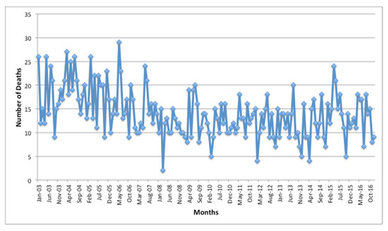
Figure 1.
Number of deaths by respiratory diseases per studied months.
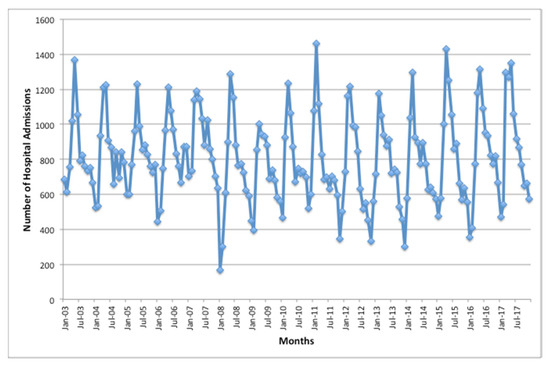
Figure 2.
Number of hospital admissions for respiratory diseases per studied months.
The computational step involved the 11 aforementioned input variables, and the desired signals (target) were mortality or morbidity. We applied the variables selection method (Mutual Information Filter and Wrapper), together with the three neural models previously described: MLP, ELM, and ESN. Additionally, we evaluated the performance considering all inputs at the same time. The adopted performance metrics were the Mean Square Error (MSE), the Mean Absolute Error (MAE), and the Mean Absolute Percentage Error (MAPE) [42].
The data were divided into three sets:
- (a)
- Considering mortality for respiratory diseases as a target:
- Training: from January 2003 to December 2010 (8 years/96 samples);
- Validation: from January 2011 to December 2013 (3 years/36 samples);
- Test: from January 2014 to December 2016 (3 years/36 samples).
- (b)
- Considering morbidity (hospital admissions) for respiratory diseases as a target:
- Training: from January 2003 to December 2011 (9 years/108 samples);
- Validation: from January 2012 to December 2014 (3 years/36 samples);
- Test: from January 2015 to December 2017 (3 years/36 samples).
The deseasonalization procedure was applied to the following variables (using Equation (1)) due to their monthly seasonal behavior: morbidity, gasoline consumption, diesel consumption, PM10, NOx, O3, SO2, and CO concentrations. The other variables (mortality, ethanol consumption, number of electric/ hybrid vehicles, and mileage round) were only stationarized, using Equation (6).
The models’ performance is summarized in Table 1, “WRP” being the acronym to Wrapper, “MI” being Mutual Information, “All” the use of all inputs, and “NN” the number of neurons in the neural models’ hidden layer. The achieved values are the mean of 30 independent simulations and the best performances are highlighted in bold. The number of neurons was defined empirically by previous tests, initiating with three, then five and after that with an increase by increments of five until reaching 200 units. In addition, all the ANN present only one hidden layer [57].

Table 1.
Computational results for respiratory diseases using artificial neural networks.
Finally, we applied the Friedman’s test with a 95% confidence interval. All cases achieved p-values very close to zero (below 0.01). This allows admitting that the obtained results are significantly different when changing the neural model.
To assure that using ANN is the best choice, we applied a Generalized Linear Model (GLM) with Poisson Regression for the morbidity case. As expected, the achieved errors were higher than all neural models (MSE = 170,424.47, MAE = 346.87, and MAPE = 57.69).
The computational results allow analyzing many aspects of the neural networks application to this problem.
In all cases, the use of the deseasonalization increases the neural models’ performance. This indicates the relevance of withdrawing the seasonal data component. As discussed, this work performed nonlinear mapping, as we are using exogenous variables to estimate mortality and morbidity. However, studies that involve time series forecasting using only endogenous inputs, addressed this approach many times, since some linear models, like the AutoRegressive Integrated Moving Average (ARIMA), cannot work with seasonal variables [42].
Regarding the addressed variable selection methods, it is important to mention that the use of mutual information withdraws the following variables of the subset: number of electric and hybrid cars, CO, and SO2. However, it did not bring a performance gain, since in all scenarios the results were worse. Considering the wrapper methodology, although we do not show it numerically, the computational effort and the time spent to finish the simulations were many times higher than in the other cases.
Additionally, we need to highlight that, in spite of the variable selection methods excluding the low fleet of electric and hybrid cars (roughly 0.03%) from the analysis, this input variable should be considered in future studies, as its production and use is being encouraged.
Due to the conflicting results based on distinct error metrics to evaluate the performance, we adopted MSE as the most important one, because ANN tries to decrease MSE during the training process [24].
With that in mind, the Extreme Learning Machines (ELM) achieved the best overall results for morbidity, with a Mean Square Error (MSE) of 25,684.56, and the Echo State Network (ESN) reached the best performance for mortality (MSE of 22.80), both using deseasonalization and all inputs. These are important results because those architectures (the Unorganized Machines) are relatively new and the adjustment of their free parameters is simple and fast, requiring only a short time to be trained. As discussed in Section 2, such architectures do not perform an iterative process during training tasks, unlike the classic MLP.
In the same way, withdrawing any variables is not an advantage. Therefore, we can state that all of them are important and must be considered.
Unfortunately, there is no consensus regarding what is the best approach to estimate air pollution health risks [16,20,25,26,41], as it depends on the database behavior. Even for conventional regressions, such as the Generalized Linear Model, the best distribution may depend on the dataset, as reported by Ardiles et al. [58]. Therefore, the best results for mortality and morbidity being achieved by different models was expected.
Figure 3 presents the boxplot of the MSE to the three neural models, considering deseasonalization and all inputs, for mortality (number of deaths) (Figure 3a) and morbidity (number of hospital admissions) (Figure 3b). In both cases, the neural model achieving the best results also presents the smallest dispersion. It is another indicative that the models are suitable for these problems.
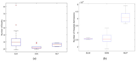
Figure 3.
Boxplot of MSE of the best scenarios: (a) mortality and (b) morbidity.
Figure 4 shows the best results achieved for the addressed data, comprising all inputs with deseasonalization. Figure 4a shows the observed and estimated results due to mortality (number of deaths) in the test set, and Figure 4b shows the same outputs due to morbidity (number of hospital admissions) in the test set, demonstrating that the models are suitable to such problems. It is clear that the models predicted morbidity better than mortality, as the last one is a result of long-term exposure, more dependent on innumerous factors, such as people’s life style and genetics. Another reason may be the patterned behavior of the morbidity series.
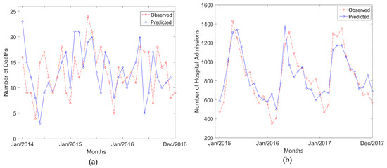
Figure 4.
Best found predictions compared to the observed data: (a) mortality and (b) morbidity.
4. Conclusions
Decision-makers should base their future actions on analyses that are able to relate a set of variables that may have influence on critical issues. In this context, we used Artificial Neural Networks (ANN) as a tool that presented good performance on forecasting the impacts of road transport variables, including air pollutants concentration and fuel consumption, on São Paulo’s population’s health. The results of our work will guide the government regarding future legislations and public policies aiming to warranty and improve the health system.
In spite of the a low relation between some inputs and the outputs, showed by the variable selection methods, the results demonstrated that withdrawing any variables is disadvantageous. Therefore, we may assume that all considered variables are important and must be considered. Even electric vehicles, accounting for only 0.03% of the vehicles fleet in São Paulo city, cannot be discarded, showing the importance of public policies in favor of electric cars.
The analysis showed that the Extreme Learning Machines (ELM) achieved the best overall results on morbidity, and the Echo State Network (ESN) reached the best performance on mortality, both using deseasonalization and all inputs. These are important results because the considered architectures are relatively new and the adjustment of their free parameters is simple and efficient, requiring only a short time to be trained.
In future research, it is important to develop an easy-to-use software including ELM and ESN and other neural models, even adding regression models to facilitate decision makers’ applications.
Considering the United Nations’ sustainable development goals (SDG) [59], which are actions needed in order to change the world, our study makes an important contribution, as it shows some relevant aspects that, if controlled or reduced, may decrease mortality and respiratory diseases related to air pollution (SDG 3—good health and well-being), and also mentions the importance of encouraging the use of electric cars and renewable fuels through tax incentive laws, increasing the participation of Brazil in the global energy matrix (SDG 7—affordable and clean energy). Therewith, we will contribute to reaching the goal of making cities and people conglomerates inclusive, secure, resilient, and sustainable (SDG11—sustainable cities and communities).
Author Contributions
Conceptualization, H.S., Y.K., D.M.d.G.C., and Y.d.S.T.; methodology, H.S. and Y.d.S.T.; software, H.S. and J.T.B.; formal analysis, Y.d.S.T. and T.A.A.; investigation, H.S., J.T.B., and Y.d.S.T.; resources, H.S.; data curation, Y.K. and D.M.d.G.C.; writing—original draft preparation, H.S., Y.K., and D.M.d.G.C.; writing—review and editing, Y.d.S.T. and T.A.A.; visualization, T.A.A.; supervision, H.S. and Y.d.S.T.; project administration, H.S.; funding acquisition, H.S. All authors have read and agreed to the published version of the manuscript.
Funding
This research was funded by the National Council for Scientific and Technological Development (CNPq), grant number 405580/2018-5, and the APC was funded by DIRPPG/UTFPR/PR.
Conflicts of Interest
The authors declare no conflict of interest.
References
- Landrigan, P.J.; Fuller, R.; Acosta, N.J.R.; Adeyi, O.; Arnold, R.; Basu, N.; Baldé, A.B.; Bertollini, R.; Bose-O’Reilly, S.; Boufford, J.I.; et al. The Lancet Commission on pollution and health. Lancet 2018, 391, 462–512. [Google Scholar] [CrossRef]
- Zhu, Y.; Hinds, W.C.; Kim, S.; Shen, S.; Sioutas, C. Study of ultrafine particles near a major highway with heavy-duty diesel traffic. Atmos. Environ. 2002, 36, 4323–4335. [Google Scholar] [CrossRef]
- Zheng, M.; Salmon, L.G.; Schauer, J.J.; Zeng, L.; Kiang, C.S.; Zhang, Y.; Cass, G.R. Seasonal trends in PM2.5 source contributions in Beijing, China. Atmos. Environ. 2005, 39, 3967–3976. [Google Scholar] [CrossRef]
- Zielinska, B.; Sagebiel, J.; Arnott, W.P.; Rogers, C.F.; Kelly, K.E.; Wagner, D.A.; Lighty, J.S.; Sarofim, A.F.; Palmer, G. Phase and size distribution of polycyclic aromatic hydrocarbons in diesel and gasoline vehicle emissions. Environ. Sci. Technol. 2004, 38, 2557–2567. [Google Scholar] [CrossRef] [PubMed]
- Reşitoğlu, Í.A.; Altinişik, K.; Keskin, A. The pollutant emissions from diesel-engine vehicles and exhaust after treatment systems. Clean Technol. Environ. 2015, 17, 15–27. [Google Scholar] [CrossRef]
- Borillo, G.C.; Tadano, Y.S.; Godoi, A.F.L.; Pauliquevis, T.; Sarmiento, H.; Rempel, D.; Yamamoto, C.I.; Marchi, M.R.R.; Potgieter-Vermaak, S.; Godoi, R.H.M. Polycyclic Aromatic Hydrocarbons (PAHs) and nitrated analogs associated to particulate matter emission from a Euro V-SCR engine fuelled with diesel/biodiesel blends. Sci. Total Environ. 2018, 644, 675–682. [Google Scholar] [CrossRef] [PubMed]
- BRASIL—Ministério da Economia, Indústria, Comércio Exterior e Serviços. Medida Provisória nº 843, de 05 de julho de 2018. In Estabelece requisitos obrigatórios para a comercialização de veículos no Brasil, institui o Programa Rota 2030—Mobilidade e Logística e dispõe sobre o regime tributário de autopeças não produzidas; Diário Oficial da União: Brasília, Brazil, 2018. [Google Scholar]
- Andrade, M.F.; Kumar, P.; Freitas, E.D.; Ynoue, R.Y.; Martins, J.; Martins, L.D.; Nogueira, T.; Perez-Martinez, P.; Miranda, R.M.; Albuquerque, T.; et al. Air quality in the megacity of São Paulo: Evolution over the last 30 years and future perspectives. Atmos. Environ. 2017, 159, 66–82. [Google Scholar] [CrossRef]
- World Health Organization (WHO), Regional Office for Europe. Evolution of WHO Air Quality Guidelines: Past, Present and Future, 1st ed.; WHO Regional Office for Europe: Copenhagen, Denmark, 2017. [Google Scholar]
- Andrade, M.F.; Miranda, R.M.; Fornaro, A.; Kerr, A.; Oyama, B.; Andre, P.F.; Saldiva, P. Vehicle emissions and PM2.5 mass concentrations in six brazilian cities. Air Qual. Atmos. Health 2012, 5, 79–88. [Google Scholar] [CrossRef] [PubMed]
- Miranda, R.M.; Andrade, M.F.; Fornaro, A.; Astolfo, R.; de Andre, P.A.; Saldiva, P.A. Urban air pollution: A representative survey of PM2.5 mass concentrations in six Brazilian cities. Air Qual. Atmos. Health 2012, 5, 63–77. [Google Scholar] [CrossRef]
- Bell, M.L.; Davis, D.L.; Gouveia, N.; Borja-Aburto, V.H.; Cifuentes, L.A. The avoidable health effects of air pollution in three Latin American cities: Santiago, São Paulo, and Mexico City. Environ. Res. 2006, 100, 431–440. [Google Scholar] [CrossRef]
- IBGE—Brazilian Institute of Geography and Statistics (in Portuguese: Instituto Brasileiro de Geografia e Estatística). Censo 2010. 2016. Available online: https://censo2010.ibge.gov.br/ (accessed on 22 August 2018).
- United Nations, Department of Economic and Social Affairs, Population Division. The world’s cities in 2016—data booklet (ST/ESA/SER.A/392). 2016. Available online: http://www.un.org/en/development/desa/population/publications/pdf/urbanization/the_worlds_cities_in_2016_data_booklet.pdf (accessed on 22 August 2018).
- Bakonyi, S.M.C.; Danni-Oliveira, I.M.; Martins, L.C.; Braga, A.L.F. Air pollution and respiratory diseases among children in the city of Curitiba, Brazil (in Portuguese). Rev. Saúde Pública 2004, 38, 695–700. [Google Scholar] [CrossRef] [PubMed]
- Kassomenos, P.; Petrakis, M.; Sarigiannis, D.; Gotti, A.; Karakitsios, S. Identifying the contribution of physical and chemical stressors to the daily number of hospital admissions implementing an artificial neural network model. Air Qual. Atmos. Health 2011, 4, 263–272. [Google Scholar] [CrossRef]
- Nardocci, A.C.; Freitas, C.U.; Ponce de Leon, A.C.M.; Junger, W.L.; Gouveia, N.C. Air pollution and respiratory and cardiovascular diseases: A time series study in Cubatão, São Paulo State, Brazil (in Portuguese). Cad. Saúde Pública 2013, 29, 1867–1876. [Google Scholar] [CrossRef] [PubMed]
- Vanos, J.K.; Hebbern, C.; Cakmak, S. Risk assessment for cardiovascular and respiratory mortality due to air pollution and synoptic meteorology in 10 Canadian cities. Environ. Pollut. 2014, 185, 322–332. [Google Scholar] [CrossRef] [PubMed]
- Çapraz, O.; Deniz, A.; Dogan, N. Effect of air pollution on respiratory hospital admissions in Ístanbul, Turkey, 2013 to 2015. Chemosphere 2017, 181, 544–550. [Google Scholar] [CrossRef]
- Polezer, G.; Tadano, Y.S.; Siqueira, H.V.; Godoi, A.F.L.; Yamamoto, C.I.; André, P.A.; Pauliquevis, T.; Andrade, M.F.; Oliveira, A.; Saldiva, P.H.N.; et al. Assessing the impact of PM2.5 on respiratory disease using artificial neural networks. Environ. Pollut. 2018, 235, 394–403. [Google Scholar] [CrossRef]
- Borillo, G.C.; Tadano, Y.S.; Godoi, A.F.L.; Santana, S.S.M.; Weronka, F.M.; Penteado Neto, R.A.; Rempel, D.; Yamamoto, C.I.; Potgieter-Vermaak, S.; Potgieter, J.H.; et al. Effectiveness of selective catalytic reduction systems on reducing gaseous emissions from an engine using diesel and biodiesel blends. Environ. Sci. Technol. 2015, 49, 3246–3251. [Google Scholar] [CrossRef]
- Nie, Y.M.; Ghamami, M.; Zockaie, A.; Xiao, F. Optimization of incentive polices for plug-in electric vehicles. Transport. Res. B Meth. 2016, 84, 103–123. [Google Scholar] [CrossRef]
- Patra, A.K.; Gautam, S.; Kumar, P. Emissions and human health impact of particulate matter from surface mining operation—A review. Environ. Technol. Innov. 2016, 5, 233–249. [Google Scholar] [CrossRef]
- Haykin, S.O. Neural Networks and Learning Machines, 2nd ed.; Prentice-Hall: Toronto, ON, Canada, 2009. [Google Scholar]
- Siqueira, H.; Boccato, L.; Attux, R.; Lyra, C. Unorgnized machines for seasonal streamflow series forecasting. Int. J. Neural Syst. 2014, 24, 1430009–1430016. [Google Scholar] [CrossRef]
- Siqueira, H.; Boccato, L.; Luna, I.; Attux, R.; Lyra, C. Performance analysis of unorganized machines in streamflow forecasting of Brazilian plants. Appl. Soft Comp. 2018, 68, 494–506. [Google Scholar] [CrossRef]
- Feng, X.; Li, Q.; Zhu, Y.; Hou, J.; Jin, L.; Wang, J. Artificial neural networks forecasting of PM2.5 pollution using air mass trajectory based geographic model and wavelet transformation. Atmos. Environ. 2015, 107, 118–128. [Google Scholar] [CrossRef]
- Mishra, D.; Goyal, P.; Upadhyay, A. Artificial intelligence based approach to forecast PM2.5 during haze episodes: A case study of Delhi, India. Atmos. Environ. 2015, 102, 239–248. [Google Scholar] [CrossRef]
- Franceschi, F.; Cobo, M.; Figueredo, M. Discovering relationships and forecasting PM10 and PM2.5 concentrations in Bogotá, Colombia, using artificial neural networks, principal component analysis, and k-means clustering. Atmos. Pollut. Res. 2018, 9, 912–922. [Google Scholar] [CrossRef]
- Cabaneros, S.M.; Calautit, J.K.; Hughes, B.R. A review of artificial neural network models for ambient air pollution prediction. Environ. Modell. Softw. 2019, 119, 285–304. [Google Scholar] [CrossRef]
- Feng, R.; Zheng, H.-J.; Gao, H.; Zhang, A.-R.; Huang, C.; Zhang, J.-X.; Kun, L.; Fan, J.-R. Recurrent neural network and random forest for analysis and accurate forecast of atmospheric pollutants: A case study in Hangzhou, China. J. Clean. Prod. 2019, 231, 1005–1015. [Google Scholar] [CrossRef]
- Ma, J.; Ding, Y.; Cheng, J.C.P.; Jiang, F.; Wan, Z. A temporal-spatial interpolation and extrapolation method based on geographic long short-term memory neural network for PM2.5. J. Clean. Prod. 2019, 237, 117729. [Google Scholar] [CrossRef]
- Gardner, M.W.; Dorling, S.R. Artificial neural networks (the multilayer perceptron)—A review of applications in the atmospheric sciences. Atmos. Environ. 1998, 32, 2627–2636. [Google Scholar] [CrossRef]
- Nagendra, S.M.S.; Khare, M. Modelling urban air quality using artificial neural network. Clean. Technol. Environ. 2005, 7, 116–126. [Google Scholar] [CrossRef]
- Zolghadri, A.; Cazaurang, F. Adaptive nonlinear state-space modelling for the prediction of daily mean PM10 concentrations. Environ. Model. Softw. 2006, 21, 885–894. [Google Scholar] [CrossRef]
- Fernando, H.J.S.; Mammarella, M.C.; Grandoni, G.; Fedele, P.; Di Marco, R.; Dimitrova, R.; Hyde, P. Forecasting PM10 in metropolitan areas: Efficacy of neural networks. Environ. Pollut. 2012, 163, 62–67. [Google Scholar] [CrossRef] [PubMed]
- Wang, Q.; Liu, Y.; Pan, X. Atmosphere pollutants and mortality rate of respiratory diseases in Beijing. Sci. Total Environ. 2008, 391, 143–148. [Google Scholar] [CrossRef] [PubMed]
- Fontes, T.; Silva, L.M.; Pereira, S.R.; Coelho, M.C. Application of artificial neural networks to predict the impact of traffic emissions on human health. Lect. Notes Comput. Sci. 2013, 8154, 21–29. [Google Scholar] [CrossRef]
- Sundaram, N.M.; Sivanandam, S.N.; Subha, R. Elman neural network mortality predictor for prediction of mortality due to pollution. Int. J. Appl. Eng. Res. 2016, 11, 1835–1840. [Google Scholar]
- Tadano, Y.S.; AntoniniAlves, T.; Siqueira, H.V. Unorganized machines to predict hospital admissions for respiratory diseases. In Proceedings of the IEEE Latin American Congress on Computational Intelligence, Cartagena de Las Índias, Colombia, 2–4 November 2016. [Google Scholar]
- Araujo, N.A.; Belotti, J.T.; Antonini Alves, T.; Tadano, Y.S.; Siqueira, H. Ensemble method based on Artificial Neural Networks to estimate air pollution health risks. Environ. Model. Softw. 2020, 123, 104567. [Google Scholar] [CrossRef]
- Box, G.E.P.; Jenkins, G.M.; Reinsel, G.C.; Ljung, G.M. Time Series Analysis: Forecasting and Control, 5th ed.; John Wiley & Sons: Hoboken, NJ, USA, 2015. [Google Scholar]
- Luna, I.; Ballini, R. Top-down strategies based on adaptive Fuzzy rule-based systems for daily time series forecasting. Int. J. Forecast. 2011, 27, 708–724. [Google Scholar] [CrossRef]
- Siqueira, H.; Boccato, L.; Attux, R.; Lyra, C. Echo state networks and extreme learning machines: A comparative study on seasonal streamflow series prediction. Lect. Notes Comp. Sc. 2012, 7664, 491–500. [Google Scholar] [CrossRef]
- Guyon, I.; Elisseeff, A. An introduction to variable and feature selection. J. Mach. Learn. Res. 2003, 3, 1157–1182. [Google Scholar] [CrossRef][Green Version]
- Villanueva, W.J.P.; Santos, E.P.; Von Zuben, F.J. Data partition and variable selection for time series prediction using wrappers. In Proceedings of the IEEE International Joint Conference on Neural Networks, Vancouver, BC, Canada, 16–21 July 2006. [Google Scholar]
- Cover, T.M.; Thomas, J.A. Elements of Information Theory, 1st ed.; John Wiley& Sons: New York, NY, USA, 1991. [Google Scholar]
- Huang, G.-B.; Zhu, Q.-Y.; Siew, C.-K. Extreme learning machine: Theory and applications. Neurocomputing 2006, 70, 489–501. [Google Scholar] [CrossRef]
- Castro, L.N. Fundamentals of Natural Computing: Basic Concepts, Algorithms and Applications, 1st ed.; Chapman & Hall: Boca Raton, FL, USA, 2006. [Google Scholar]
- Huang, G.-B.; Zhu, Q.-Y.; Siew, C.K. Extreme learning machine: A new learning scheme of feedforward neural networks. In Proceedings of the IEEE International Joint Conference on Neural Networks, Budapest, Hungary, 25–29 July 2004. [Google Scholar]
- Jaeger, H. The Echo State Approach to Analyzing and Training Recurrent Neural Networks; Tech. Rep. GMD Report 148; German National Research Center for Information Technology: Bremem, Germany, 2001. [Google Scholar]
- Jaeger, H. Short Term Memory in Echo State Networks; Tech. Rep. GMD Report 152; German National Research Center for Information Technology: Bremem, Germany, 2002. [Google Scholar]
- DENATRAN—National Traffic Department (in Portuguese: Departamento Nacional de Trânsito). Relatórios estatísticos. 2019. Available online: http://www.denatran.gov.br/estatistica (accessed on 10 February 2019).
- CETESB—Environmental Company of São Paulo State (in Portuguese: Companhia Ambiental do Estado de São Paulo). Qualidade do ar: Relatórios. 2018. Available online: http://cetesb.sp.gov.br/ar/qualar/ (accessed on 15 May 2018).
- ANP—National Agency of Petroleum, Natural Gas, and Biofuels (in Portuguese: Agência Nacional do Petróleo, Gás Natural e Biocombustíveis). Estatísticas de distribuição para varejistas. 2018. Available online: http://www.anp.gov.br/ (accessed on 16 July 2018).
- DataSUS—Informatics Department of the Unified Health System (in Portuguese: Departamento de Informática do Sistema Único de Saúde). Sistema de informação sobre mortalidade e morbidade. 2018. Available online: http://datasus.saude.gov.br/informacoes-de-saude/tabnet (accessed on 22 August 2018).
- Cybenki, G. Aproximation by superpositions of a sigmoidal fuction. Math. Control Signal. 1989, 2, 303–314. [Google Scholar] [CrossRef]
- Ardiles, L.G.; Tadano, Y.S.; Costa, S.; Urbina, V.; Capucim, M.N.; Silva, I.; Braga, A.; Martins, J.A.; Martins, L.D. Negative Binomial regression model for analysis of the relationship between hospitalization anda ir pollution. Atmos. Pollut. Res. 2018, 9, 333–341. [Google Scholar] [CrossRef]
- United Nations. Sustainable Development Goals: Knowledge Platform. 2019. Available online: https://sustainabledevelopment.un.org/ (accessed on 10 February 2020).


© 2020 by the authors. Licensee MDPI, Basel, Switzerland. This article is an open access article distributed under the terms and conditions of the Creative Commons Attribution (CC BY) license (http://creativecommons.org/licenses/by/4.0/).