Abstract
The development of new energy in developing areas should not only consider the effect on local economic growth, but also give some attention to its spillover effect for economic growth in neighboring areas and take a new path of cluster-style development and cooperative governance. On the basis of Moran’s I and the Spatial Dubin Model (SDM), this paper analyzes the spatial spillover effect of new energy development on economic growth of 21 developing areas in China from 2000 to 2017. The results show that: (1) According to the Moran’s I, there are significant economic agglomeration characteristics in the spatial distributions among different areas in the study area. (2) A comparative study using the mixed Ordinary Least Squares (OLS) method and SDM shows that new energy has a negative spillover effect on the economic growth of neighboring areas when considering spatial factors, but this negative effect is underestimated in the mixed OLS method. (3) In addition to the core explanatory variable, the spatial spillover effect of new energy on economic growth is also affected by control variables, but the degree of impact varies. The results imply that some effective policy measures, such as sustainable development mechanisms, industrial distribution, and comparative innovation, should be taken to encourage new energy development for the high quality growth in developing areas on the national, regional, and global scale.
1. Introduction
What is the definition of energy? What are the classifications of energy? Generally speaking, energy refers to the general name of materials that can produce various kinds of energy or work, and can be divided into primary energy and secondary energy (Figure 1). Primary energy includes traditional fossil energy and new energy. Coal, oil, and natural gas are the core of traditional fossil energy and the foundation of global energy. New energy refers to various forms of energy other than traditional fossil energy, including those that are being developed and utilized, but have not yet been commonly used, such as solar, wind, geothermal, ocean, and biological energy, etc., which are the new directions of global energy development in the future and also the focus of this paper. Secondary energy refers to the direct or indirect conversion of primary energy into other types and forms of energy resources. The secondary energy is not analyzed as it is not in the scope of this paper.
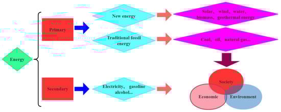
Figure 1.
Energy classification.
Energy is an important basic resource for social and economic development [1]. Since the Industrial Revolution in 1840, traditional fossil energy resources have been consumed severely with the increasing energy demand worldwide. Meanwhile, the global ecological environment has been deteriorating due to the greenhouse effect and global warming [2], and the sustainable development of human society has been seriously threatened. According to the British Petroleum (BP) Statistical Review of World Energy 2018, in 2017, global primary energy demands increased by 2.9%; carbon dioxide emissions increased by 2.0% and reached 600 million tons. In the structure of world energy, coal, oil, and natural gas are still the main sources of power to drive global economic development, although new energy production has increased significantly, but still accounts for a small proportion in the world energy structure [3]. Owing to the massive use of fossil energy and neglect of environmental protection, environmental pollution incidents have occurred frequently, and the sustainability of the world economy is getting worse. Therefore, accelerating the transformation and reform of the energy consumption structure (ECS) and developing new energy have gradually become the universal consensus and concerted action of countries around the world [4].
Energy and economic growth are closely linked. As the largest developing country in the world, since the Reform and Opening-Up was launched in 1978, China’s energy production and consumption capacity has continuously improved; it has already become the world’s largest energy producer and consumer. From 1978 to 2017, China’s total primary energy production increased from 630 million tons of standard coal to 3.59 billion tons of standard coal. The proportion of coal and new energy consumption was adjusted from 70.7% and 3.4% to 60.4% and 13.8%, respectively. The average annual energy consumption per unit of Gross Domestic Product (GDP) has fallen by 4% [5]. At the same time, the development and utilization of fossil energy has caused carbon and nitrogen oxide emissions to exceed standards. For example, in 2017, the areas of acid rain in China reached 620,000 square kilometers, accounting for 6.4% of the country’s land areas. Average national haze days were 27.5 days. Air quality indexes such as PM2.5 and PM10 were 43 μg/m3 and 75 μg/m3 [6,7]. This indicates that China’s economy is highly dependent on coal and other traditional fossil energies; at the same time, unreasonable use of resources has caused severe damage to the ecological environment. The quality of economic development needs to be improved.
As China’s economy enters a new era, high-quality development is becoming the most distinctive economic feature. High-quality economic development is inseparable from high-quality development of energy. The report of the 19th National Congress of the Communist Party of China (CPC) pointed out that China’s economy has been transitioning from a phase of rapid growth to a stage of high-quality development; energy, especially new energy, must be placed in the important position of the reform of the Ecological Civilization and Beautiful China Construction [8]. In this context, particularly in the face of the actual pressure created by environmental pollution and energy shortage, it is an urgent task for China’s developing areas to seek and utilize new energy.
The need for economic development in developing areas is strong. There are two prominent economic characteristics of the developing areas. One includes the vast areas and large population, which are far from the developed eastern coastal areas. Second, there are abundant new energy resource reserves, but the level of development and utilization is not high, and resources are wasted seriously. According to the National Bureau of Statistics (NBS), there are 22 provinces in China’s developing areas, including Guizhou, Gansu, Yunnan, Inner Mongolia, Shaanxi, Sichuan, Guangxi, Xinjiang, Hunan, Anhui, Hubei, Shanxi, Qinghai, Heilongjiang, Henan, Hebei, Jilin, Ningxia, Chongqing, Hainan, Tibet, and Jiangxi. The land areas cover 7.814 million square kilometers, accounting for 81.4% of the total land area. The population is 748 million, accounting for 53.43% of the country. At the same time, the per capita GDP of developed areas along the eastern coast is 1.8 times that of developing areas. Beyond that, water, solar, and wind energy account for 72%, 70%, and 65%, respectively. It is the most important new energy base in China. Therefore, high-quality economic development in developing areas must be based on its own new energy endowment and unique location advantages, be guided by national major strategies, and take a new path of cluster-style development and cooperative governance.
The remainder of the paper is structured as follows: A brief review of energy economy is made in Section 2. Section 3 presents the study area, variables, data sources, and models. Empirical results are presented in Section 4. Section 5 and Section 6 provide discussions, some key conclusions, and policy implications.
2. Literature Review
Research on the relationship between energy and economic growth originates from the western oil crisis in the 1970s [9]. After 50 years of intensive research, scholars around the word have conducted numerous discussions on the multi-dimensional coupling between traditional energy consumption, carbon emissions, and economic development from different perspectives.
From the perspective of theoretical research, the main theoretical foundations include the environmental Kuznets curve theory (EKC), ecological footprint (EF) theory, and control economics (CE) theory. Energy covers all aspects of social and economic life, so it is closely related to environmental protection, ecological governance, and industrial economy. For a long time, it has been the focus of research and attention of global scholars, which has led to many influential research results in theoretical research. For instance, Fodha and Zaghdoud [10] use the EKC theory to empirically analyze the dynamic relationship between carbon emissions and regional economic growth. Baz et al. [11] examine the impacts of energy consumption and economic growth on environmental quality in Pakistan using the EF theory. In order to explore whether energy conservation behavior has an impact on households, Lundgren and Schultzberg [12] analyze energy-efficient behavior on the basis of the CE theory in high-income, middle-income, and low-income households in Sweden. Their results show that different levels of energy-efficient behavior do not really have any impact on the actual consumption levels of electricity. Kraft and Kraft [13] prove that GDP and energy consumption have a one-way causal relationship, and thus open a new direction in the field of energy consumption economy research.
In terms of new energy, some scholars also have conducted substantive theoretical research. According to Kobos et al. [14], they find that production costs and research and development (R&D) investment have a decisive impact on new energy technology innovation. Compared with traditional energy, Timilsina et al. [15] point out that the cost of solar energy resource development has been reduced in recent years, but its cost is still higher than that of traditional energy. Therefore, governments should accelerate the development and utilization of energy resources through sustainable policy support. With the improvement of the quality of economic and social development, Bloch et al. [16] believe that the demand for energy has been increasing, especially for new energy. Chen [17] proposes that the transformation and upgrading of China’s new energy industry should make a policy innovation and industrial structure adjustment through market-oriented reform. Based on the field survey of 409 households in four provinces of China, Qiu et al. [18] conclude that factors such as household economic level, labor price, and household demographic characteristics have a significant impact on China’s rural new energy consumption. Liu [19] conducts a critical analysis of China’s new-energy-related laws and policy measures. Soytas and Sari [20] argues that energy consumption has a positive effect on economic growth to a certain extent through an analysis with an energy dataset of five countries from 1950 to 1992.
From the perspective of models and methods, based on the above theoretical research, abundant empirical research on energy and economic growth, especially the spatial spillover effect of new energy development on economic growth, has been carried out in some literatures. By considering spatial spillover effect, Balado-Naves et al. [21] collect panel data of 173 countries over the period of 1990–2014, and reveal that every 1% increase in new energy consumption in a country leads to the level of green development in neighboring countries increasing by 2.1%. Shuai et al. [22] discover that, for the countries at high-income (HI) level, upper-middle-income (UMI), lower-middle-income (LMI), and low-income (LI) levels, impact factors such as population, affluence, and technology on carbon emission have different effects when analyzed by the Stochastic Impacts and Regression on Population, Affluence, and Technology (STIRPAT) models with panel data of 125 countries over the period of 1990–2011 from the perspective of spatial spillover. By adopting panel data unit-root and cointegration tests as well as Granger non-causality tests relying on the system Gaussian Mixture Model (GMM) estimator, Magnani and Vaona [23] document that new energy generation has a positive spillover effect on economic growth at the regional level in Italy. Due to the effect of energy potential similarity and knowledge spillovers, Shahnazi and Shahnazi [24] insist that one important variable for new energy production is the spatial spillover of new energy production for neighboring countries. Hao et al. [25] conduct empirical research of EKC by employing a spatial econometric model and provincial per capita energy consumption as well as per capita electricity consumption.
In addition to energy economics, the spatial spillover model is also used in other socioeconomic studies. With the help of modeling knowledge spillover effects, Stejskal and Hajek [26] propose a new perspective on the evaluation of the contributions of high-tech industries in the Czech Republic using moderated and mediated analysis. When hosting mega-events such as the Olympic Games, Kim and Kang [27] suggest that walking routes or public transportation systems should be well organized, because these can contribute to enhancing spillover effects versus car rental system developments. Zafra-Gómez et al. [28] find that certain forms of public services in the region have a spatial spillover effect on the cost of providing the same public services in neighboring cities. Yu [29] explores the regional imbalance of China’s provincial energy intensity and the spatial spillover effect of energy intensity among provinces. For the purpose of estimating the drivers of energy intensity in China, Jiang et al. [30] utilize the Spatial Dubin Error Model and panel data of 29 provinces for the period 2003–2011, and discover an inverted U-shaped relationship between energy intensity and income. Among them, ten provinces along the eastern coast have passed the turning point of 29,673 yuan, while the other 19 provinces reached the turning point ranges between 8.3 and 21.8. Under the gradient economic development mode, Huang et al. [31] prove that carbon emissions have strong spatial dependence and convergence across regions.
A spatial spillover model is not the only way to study the relationship between energy consumption and economic growth. By using co-integration analysis, the Value-at-Risk (VAR) error correction model, Granger causality test, and the impulse response methods, Ma and Ye [32] discover the long-term equilibrium relationship and non-Granger causality between energy consumption and economic growth with the data of Shaanxi province from 1978 to 2014. Similarly, Jian et al. [33] examine the effects of economic growth, financial development, and energy consumption on carbon dioxide emission in China. Pereira and Pereira [34] estimate the impact of carbon dioxide emissions from fossil fuel combustion activities on economic activity in Portugal. Akalpler and Hove [35] use the Autoregressive-Distributed Lag (ARDL) model to analyze the effects of carbon dioxide emissions, energy use, gross fixed capital formation, GDP per capita, exports, and imports on Indian economic growth. The Belt and Road is an important energy transportation channel; Qi et al. [36] adopt Data Envelopment Analysis (DEA) to calculate the Total Factor Energy Efficiency (TFEE) of the Belt and Road Initiative (BRI) countries, and investigate heterogeneous beta-convergence in energy efficiency of BRI counties and its factors. In addition, some scholars have also conducted abundant research about energy consumption and economic growth, e.g., Li [37], Chen and Golly [38], Lin and Zhu [39], and Yang et al [40].
After the literature review, we find that: (1) In terms of theoretical research, scholars often used EKC, EF, CE, and other theories to carry out systematic research in the fields of ecological environment, technological innovation, and industrial structure adjustment, and have achieved fruitful research. These theoretical achievements have laid a solid foundation for the theoretical framework of this paper. (2) Because the spatial spillover effect model not only considers the impact of individual variables on the local economy, but also deals with the impact to the neighboring areas, the model estimation results are true and reliable, which is the advantage that other non-spatial economic models do not have. (3) Considering the characteristics of the research topic in this paper, the spatial spillover effect model can better achieve the research purpose. This is the most important reason for why we choose spatial spillover model in this paper.
Although existing literatures on the relationship between energy and economic growth have been sufficient, it is not difficult to find that scholars often focus their attention on developed areas with better economic conditions or different countries, and few focus on the developing areas in China. In particular, there is less research on new energy and economic growth by using the spatial spillover model. As is known to all, new energy is an important source for future economic development, and it is important to the economic development in China and even in the world’s developing areas. Therefore, this paper chooses China’s developing provinces as the study area, combined with panel data and spatial econometric models, to study the spillover effect of new energy development on economic growth in developing provinces; then, some policy implications are put forward. This is the original motivation for writing this paper.
3. Materials and Methods
3.1. Study Area
In this paper, the developing areas refer to the concentrated contiguous poverty-stricken areas and the locations of the national-level poverty counties beyond the area, mainly including the Qin-ba Mountains, Wu-ling Mountains, and the western Yunnan border mountains, totaling 495 national-level poverty counties and 22 provinces in China (for a specific list, see lines 86–88 in Section 1). Because of the inconsistent statistical caliber and incomplete data in Tibet, finally, this paper selects 21 developing provinces other than Tibet as the study area, and collects new-energy-related panel data of 21 developing provinces from 2000–2017.
3.2. Variables
3.2.1. Explained Variable
Real GDP per capita is an important factor for measuring a country’s economic strength. So, in this paper, real GDP per capita is chosen as the explained variable, and its calculation formula is the ratio of real GDP to permanent population.
3.2.2. Explanatory Variable
The development of new energy is an inevitable choice for the high-quality economic and social development in developing areas. So, we select the ratio of new energy consumption as the core explanatory variable in order to test the impact degree of new energy development on economic growth of the locale and its neighboring areas. The calculation formula is the proportion of clean new energy generation in the total annual power generation.
3.2.3. Control Variables
In addition to explained and explanatory variables, the economic growth in developing areas is also affected by labor, capital, investment, industry, and urbanization. Therefore, this paper selects human capital, physical capital, government investment, industrialization, and urbanization as control variables.
Human capital is an important factor for supporting high-quality economic growth in developing areas. Based on the number of employed persons in the China Population and Employment Statistical Yearbook, the calculation formula is edu = illiteracy * 2 + primary school * 6 + junior high school * 9 + senior high school * 12 + junior college or above * 16.
Physical capital refers to the total amount of capital at a certain time. Based on the research method of Zhang et al. [41], the calculation formula is Kit = Iit + (1 − δit)Kit-1. Kit is the physical capital of the ith province in year t, Iit is the ith province’s investment in year t, and δit is the fixed asset depreciation rate (δ = 9.6%).
Government investment is a necessary means for the government to carry out macro-control, which refers to the proportion of fiscal expenditure in GDP.
Industrialization is also a crucial factor in measuring the degree of economic development in a country. The calculation method is the proportion of industrial added value in GDP.
Urbanization as a key factor reflects the quality of a country’s economic development. The urbanization rate mentioned in this article refers to the ratio of urban permanent population to the total permanent population.
In brief, the above variables and their respective definitions, as well as their units of measurement, are shown in Table 1.

Table 1.
Definitions of all of the variables.
3.3. Data Sources
The dataset is a balanced panel that consists of observations for 21 provinces covering the period 2000–2017, with a sample of 378 observations. The original data of pgdp, edu, k, gi, ir, and urp were collected from the China Statistical Yearbook, China Demographic and Employment Statistical Yearbook, NBS of People’s Republic of China (P.R.C), Regional Statistical Yearbooks, and the bulletin on statistics of national economic and social development. The ratios of nec data were selected from China Energy Statistical Yearbook and China Rural Poverty Monitoring Report.
To reduce heteroscedasticity, this paper adopts a logarithmic method to deal with all variable data. For the missing data in some years, the local polynomial interpolation method is used without affecting the estimation results. The summary statistics of variables can be seen in Table 2.
Table 2.
Summary statistics of variables.
3.4. Method
Spatial autocorrelation is an analysis method that can gauge the correlation dependence among different geographical locations and give a significance test. It is called “Tobler’s First Law of Geography”. There are four spatial characteristics, which are showing high-high, low-low, low–high and high-low spatial associations [42].
3.4.1. Global Autocorrelation
In econometrics, Moran’s I, Geary’s C, Getis, and Join Count are the common methods for testing the spatial correlations between different variables. In view of the large research area, long time span, and complex variable factors, the global Moran’s I, which has a wide range of application and strong stability, is selected to test the spatial correlations of new energy development on economic growth in developing areas. The formula is shown in Equation (1) as follows:
where Yi represents the actual observation value of the i-th area; n is the sample size; Wij is the spatial weight matrix; Moran’s I∈(−1, 1). When 0 < I < 1, the larger the Moran’s I, the stronger the spatial correlation between variables. When −1 < I < 0, the lower the Moran’s I, the weaker the spatial correlation between variables. When Moran’s I = 0, this means that there is no spatial correlation and it is a random distribution.
3.4.2. Local Autocorrelation
With the purpose of analyzing the spatial differences between different regions in the study area, we introduce the local spatial autocorrelation model and use a scatter plot of Moran’s I to express its spatial agglomeration characteristics, which mainly have four modes (Table 3). Equation (2) is the calculation method.
where Ii is the local autocorrelation value. When Ii > 0 (first and third quadrant), it indicates that the research area and the neighboring areas are showing high–high or low–low agglomeration characteristics, and it is a positive correlation. When Ii < 0 (second and fourth quadrant), it indicates that the research area and its neighboring areas are showing high–low agglomeration characteristics, and it is a negative correlation. When Ii = 0, it means that there are no spatial agglomeration characteristics. n is the sample size; ?x is the means of variable indicators; Wij is the spatial weight matrix.
Table 3.
Four modes of local autocorrelation.
3.4.3. Spatial Weight Matrix
There are four kinds of spatial weight matrixes: The 0–1 matrix, economic distance matrix, geographic distance matrix, and economic–geographic nested matrix. Because this paper mainly studies the spatial spillover effect of new energy development on economic growth and quantifies the spatial spillover degrees of different variables on the economic development of a locale and its neighboring areas, the economic distance matrix is chosen as the spatial weight matrix. The economic distance matrix takes the reciprocal of the pgdp difference between the two areas as a weight to determine whether the two areas are neighboring. If the difference in the pgdp of the two areas is small, the economic gap will be small. In this case, it will be given a larger weight. If the difference gets larger, the economic gap will be large, and then it will be given a smaller weight. The formula for calculating the economic distance matrix is given in Equation (3).
where Wij represents the economic distance weight; and are the pgdp of the i province and j province; .
3.4.4. Spatial Dubin Model
Compared with other research methods, the Spatial Dubin Model (SDM) is one of the most used methods to measure the spatial spillover effect because it not only considers the spatial correlation of explanatory variables, but also lays stress on the spatial correlation of explained variables. Explained variables are affected by the local explanatory variables, and are also affected by the explanatory variables and the explained variables in neighboring areas. The analysis results are more in line with the actual situation and have more reference value. The calculation formula is shown in Equation (4).
Y is the explanatory variable; ρ represents the spatial regression coefficient; W is the spatial weight matrix; X is the explanatory variable; ln stands for the nth identity matrix; θ and β are the coefficients, α is the constant term, ε is the random error term; when θ = 0, the SDM model degenerates to the spatial lag model (SLM); when θ + ρβ = 0, the SDM model degenerates to the Spatial Error Model (SEM).
3.4.5. Direct and Indirect Effects
When the SDM is used to analyze the spatial spillover effect of new energy development on economic growth in developing areas, we cannot simply use regression coefficients to determine the relationship between the explanatory and explained variables. It needs to be further decomposed by introducing analysis methods of direct, indirect, and total effects. The calculation formulas are shown in Equations (5)–(7), as follow:
; ; is the nth identity matrix.
According to Equation (7), the direct effect formula is , indicating the impact of explanatory and control variables on the economic growth of the local area. The indirect effect formula is , indicating the spatial spillover effect of explanatory and control variables on economic growth in neighboring areas.
4. Empirical Results
4.1. Global Autocorrelation Test
In this paper, the economic distance matrix and Stata15 software are used to test the global Moran’s I of 21 developing provinces in China from 2000 to 2017 (Table 4). The results show that: From 2000 to 2017, the global Moran’s I values of the 21 provinces are all positive, the maximum value is 0.576, the minimum value is 0.551, and the p value is 0.000, all of them at the significance level of 1%. This shows that the spatial economic benefits of the 21 provinces are not random, scattered, and disordered completely; on the contrary, they have significant global spatial agglomeration characteristics.
Table 4.
Global Moran Index according to actual GDP per capita.
4.2. Local Autocorrelation Test
Local spatial autocorrelation is an important method for testing the spatial correlations of different provinces in the study area, and is often presented in the form of a Moran’s I scatter plot. In this study, Moran’s I scatter plots are chosen with significant representative features in 2002, 2007, 2012, and 2017 (Figure 2). In Figure 2, it is shown that, although the 21 developing provinces in China have obvious agglomeration correlation characteristics in the development of new energy, they also obviously have non-equilibrium characteristics in terms of internal spatial distribution. Most provinces are located in the first and third quadrants, with obvious high–high and low–low correlation characteristics.
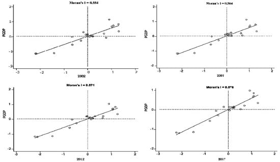
Figure 2.
Local Moran’s I scatter plot.
4.3. Spatial Dubin Model Analysis
Through the Global Moran’s I in Table 4 and Local Moran’s I scatter plot in Figure 2, it has been proven that the spatial correlations of the 21 developing provinces are significant. Therefore, it is appropriate to use the spatial econometric model for further verification and interpretation. Now, there are three econometric models to study spatial correlation: SLM, SEM, and SDM, respectively. Because the above three models have different application boundaries and scopes, it is necessary to have an adaptability test in order to choose the most effective spatial econometric model. At present, there are three adaptability test methods for spatial econometric models: Wald test, Likelihood Ratio (LR) test, and Lagrange Multiplier (LM) test. All three of these test methods are asymptotically equivalent and obey the chi square distribution with the degree of freedom as the divisor. Generally speaking, it is feasible to use any of the above methods to test large samples of data. Based on the existing literature, the Wald test and LR test are finally selected to determine which spatial econometric model is most suitable for this paper.
After the Wald and LR tests, the statistics of Wald spatial lag, LR spatial lag, Wald spatial error, and LR spatial error are 8.8223, 7.1402, 7.295, and 5.1048, respectively. All of them are at the significance level of 1%, and reject the null hypothesis of H0. Therefore, the SDM is effective.
In addition, it is a fundamental issue to choose a fixed effect or random effect when dealing with panel data. According to the Hausman test results, the p value is 0.000 at the significance level of 1%, indicating that the fixed effect model is better than the random effect model.
4.3.1. Estimation of Panel Data without Considering Spatial Factors
Before the spatial correlation analysis, it is necessary to analyze the panel data with the mixed ordinary least squares (OLS) method so as to compare with the spatial analysis results (see Table 5).
Table 5.
Mixed ordinary least squares (OLS) method estimation without considering spatial factors.
In Table 5, the elasticity coefficient of nec is 0.009287 and fails at any significance level, which indicates that the development of new energy in developing areas has a positive effect on economic growth, but not significantly. Except for government investment, the other four control variables all have positive effects on economic development, and the effects are significant.
The Durbin–Watson (DW) value is 0.3098, which means that there is autocorrelation in the residual sequence of samples. So, the Moran’s I model is used to test the spatial correlation of the residual sequences generated under the estimation of the mixed OLS method. The results show that the residual sequences are at the significance level of 1%, which indicates that there is significant spatial correlation. The LM test with no spatial lag is 50.0531 and the LM test with no spatial error is 92.8548, both at the significances level of 1%, indicating that there are spatial lag terms and spatial error terms, so it is necessary to establish the SDM.
4.3.2. Estimation of the SDM
As seen in Table 5, there are residual sequences, spatial lag, and error terms in the estimation of panel data using the mixed OLS model; this means that the above estimation results are biased, which does not satisfy the assumptions under classical linear conditions.
In order to eliminate the biased estimation results under non-spatial conditions, the SDM and the Maximum Likelihood (ML) estimation are employed to analyze the spatial correlation of the study areas (Table 6). In Table 6, under the spatial and time fixed effect, the elasticity coefficient of lnnec is 0.006448, and the t value is 0.65078; it fails at all significance levels, which indicates that the increase of proportion of nec has a positive effect on economic growth in developing areas, but the positive effect is not significant yet. The elasticity coefficient of W*lnnec is 0.00848, and the t value is 0.254935; it fails at all significance levels, which shows that the development of new energy in neighboring areas has a positive spillover effect on the local economic growth, but the positive spillover effect is not significant.
Table 6.
Estimation of the Spatial Dubin Model (SDM) of new energy development on economic growth.
Under the spatial and time fixed effect, among the control variables, the elasticity coefficient of gi is 0.058552, and the t value is 1.09463; it fails at all significance levels, which implies that government investment has a positive effect on economic growth of the locale, but the positive effect is not significant. After the spatial matrix is added, the elasticity coefficient of W*lngi is 0.245878 at the significance level of 10%, which means that the government investment in neighboring areas has a positive spillover effect on economic growth of the locale, and this positive spillover effect is also significant to the neighboring areas. In addition, the elasticity coefficients of W*lnk, W*lnir, W*lnedu, and W*lnurp are −0.015316, −0.075811, 0.115146, and 0.266693, respectively; all of them fail at all significance levels, which illustrates that the reduction of the physical capital and industrialization, as well as the increase of human capital and urbanization in neighboring areas, has a positive spillover effect on local economic growth, but it is currently not significant.
4.3.3. Verification of Direct, Indirect, and Total Effects
It is not sufficient to study the spillover effect of new energy development on economic growth only by analyzing the estimated coefficients of the SDM, so further analysis is needed. In order to more specifically reflect the effect of new energy development on economic growth, we decompose the SDM into direct effect, indirect effect, and total effect. The results are shown in Table 7.
Table 7.
Direct, indirect, and total effects of the SDM.
Under the direct effect in Table 7, the elasticity coefficient of lnnec is 0.0072925; it fails at all significance levels, which indicates that the increase of the proportion of nec can promote the economic growth of the locale, but not significantly at present. The main reasons are that, on the one hand, the increase of the proportion of nec can reduce the dependence of developing areas on traditional fossil energy, such as coal and oil, and save more investment in environmental pollution, thereby obtaining more ecological benefits. On the other hand, new energy has obvious characteristics, such as low development cost and high utilization rate, which can improve the energy consumption intensity and reduce energy consumption per unit of GDP in developing areas.
Among the control variables, the elasticity coefficients of lnk and lnir are 0.16428011 and 0.2108014, respectively, both at the significance level of 1%, which implies that the improvement of the physical capital and industrialization can significantly promote the local economic growth. The elasticity coefficient of gi is −0.0218864, but not at all significance levels, which means that the level of government investment in developing areas has a negative effect on the economic growth, and this effect is not significant.
This paper mainly studies the spatial spillover effect of new energy development on economic growth in developing areas, so indirect effect is the crucial content of this research. In the indirect effect, the elasticity coefficient of lnnec is −0.041731 at the significance level of 5%, which shows that the change of new energy consumption can potentially block economic growth of the neighboring areas by changing the spatial interaction, that is to say, it produces a negative spatial spillover effect, and this negative effect is significant.
Because new energy is a high-tech and strategic emerging industry supported by the government, especially with China’s economy entering the stage of high-quality development, it has gradually become the consensus of the whole society to eliminate traditional energy, develop new energy, and take the road of a green, low-carbon, and circular economy. To develop new energy, the central government must provide several preferential policies. This is also one of the common international practices to support the development of new energy when it has not fully developed. However, the implementation of these preferential policies will inevitably lead to fierce competition among different provinces. Once one of the local governments obtains the qualification to develop new energy, it will get several preferential policies from the upper governments. These preferential policies can not only bring a large amount of capital and technology as well as other production elements, but, at the same time, they will also cause a negative spillover effect on the economic development of neighboring areas. Thus, these cause policy bias in finance, technology, and talent at the implementation level. This is the reason for why the development of new energy will promote the economic development of the locale, but produce a negative spatial spillover effect on the neighboring areas.
The elasticity coefficient of lnedu is 0.1630871 at the significance level of 10%, which indicates that the improvement of human capital has a positive spatial spillover effect on economic growth of the neighboring areas. The main reason is that human capital produces a spillover effect through technological output and diffusion, which can drive the economic development of the neighboring areas.
The elasticity coefficients of lnk, lngi, and lnir are −0.165107, −0.244092, and −0.326521, respectively, all at the significance level of 1%, which exposes that physical capital, government investment, and industrialization have negative spatial spillover effects on the economic growth of neighboring areas, and these spillover effects are significant. For most developing areas, they are at the rising stage of industrialization owing to the lower economic development level; thus, their industrial structure, level, and quality have strong similarities to the neighboring areas. In addition, most governments carry out blind expansion and competition from the perspective of local selfish departmentalism, without thinking of a chess game and the integration of development, so as to produce a negative spatial spillover effect on the economic growth of the neighboring areas.
The elasticity coefficient of lnurp is 0.5367898 at the significance level of 1%, which shows that the improvement of urbanization will have a significant positive spatial spillover effect on the neighboring areas.
5. Discussion
From the perspective of econometrics, this paper studies the spillover effect of new energy on economic growth over the period of 2000–2017 in 21 developing areas of China. The results show that the development of new energy in developing areas presents typical spatial agglomeration characteristics when considering spatial factors. Although new energy plays a positive role in promoting economic development in one area, it will inevitably have a negative spillover effect on neighboring areas. This conclusion can not only provide theoretical support for the formulation of new energy policies and industrial structure optimization, but also provide technical guidance for China’s energy consumption structure transformation.
Compared with previous studies, the main contributions of this paper include: First, the study area is representative. Under the background of the new norm of economic development, we select 21 developing areas, including Guizhou, Yunnan, and other provinces, which are located in the central-west areas of China. These areas have been facing serious economic, resource, and environmental problems for a long time. Second, the research time period is large. The time span of this paper is 17 years in total, since the beginning of the 21st century; the time node is very special, which is relatively rare in previous literature. Third, the research perspective is novel. In the context of economic transformation and upgrading, few literatures study the relationship between new energy and economic growth from the perspective of spatial spillover. Fourth, the viewpoint based on the research results is different from other similar researches. Through the Moran’s I and the SDM, it is found that the development of new energy in developing areas has a strong spatial agglomeration characteristic, so it is necessary to realize the coordinated development through cooperative governance.
As the research samples are only for 21 provinces in China, the scope of application of the research conclusions may be limited. In the future, we will select data from other developing regions of the world for further research to strengthen our research conclusions.
6. Conclusions and Policy Implications
6.1. Conclusions
This paper explores the spatial spillover effect of new energy development on economic growth for a panel of 21 developing provinces over the period 2000–2017 by using an economic distance matrix, Moran’s I, and SDM. The conclusions are as follows:
- (1)
- The Moran’s I of the 21 developing provinces is not in a random and scattered state in the first and third quadrants, which show high–high and low–low characteristics. This shows that the development of new energy in developing areas has a strong spatial agglomeration characteristic.
- (2)
- Without considering the spatial weight matrix, the positive effect of new energy development on economic growth in developing areas is underestimated. After adding the spatial weight matrix, the positive effect is enhanced, but it produces a negative spatial spillover effect on the economic growth of neighboring areas.
- (3)
- From the perspective of control variables, the spatial spillover effects of human capital, physical capital, government investment, industrialization, and urbanization on the economic growth of neighboring areas are different. Human capital and urbanization have positive spatial spillover effects on the economic growth of the neighboring areas, while physical capital, government investment, and industrialization have negative spatial spillover effects.
6.2. Policy Implications
On the basis of the above results, several relevant and straightforward policy implications can be derived, as follows:
- (1)
- As an important new energy base in China, the development of new energy in developing areas is insufficient, and the policy system is not complete enough. Therefore, local governments in developing areas should strengthen the emphasis on new energy development, especially from the perspective of urbanization and human capital. The government should intensify policy innovation, form a long-term mechanism to support the sustainable development of new energy, and provide a great source of power for high-quality economic development in developing areas.
- (2)
- As the development of new energy in developing areas has strong spatial agglomeration characteristics and spillover effects, local governments in developing areas should increase the intensity of macro-control by optimizing the layout of the new energy industry, rationally arranging the timing of new energy development, controlling the scale of new energy development, and providing a solid foundation for the healthy development of new energy in developing areas.
- (3)
- Developing areas should combine their endowments with new energy resources, finding their own comparative advantages to develop new energy with local characteristics. This should take a differentiated development route, avoiding the problem of "homogenization" of resource development, and transforming comparative advantages into competitive advantages.
Author Contributions
Conceptualization, S.L.; methodology, J.B. and S.L.; software, J.B. and N.W.; validation, S.L. and N.W.; formal analysis, J.B.; investigation, J.B., X.L., and J.S.; resources, S.L.; data curation, J.B., N.W., and S.L.; writing—original draft, J.B.; writing—review and editing, S.L., X.L., and J.S.; visualization, X.L., J.S., and J.B.; supervision, S.L.; project administration, S.L.; funding acquisition, S.L. All authors have read and agreed to the published version of the manuscript.
Funding
This paper was supported by the National Social Science Foundation of China under Grant No.16BJY049, by the Special Fund for Basic Scientific Research of Central Colleges, China University of Geosciences (Wuhan) Grant No.CUG170105.
Acknowledgments
The authors would like to thank the anonymous reviewers for their critical comments and constructive suggestions.
Conflicts of Interest
The authors declare no conflicts of interest.
References
- Pui, K.L.; Othman, J. The influence of economic, technical, and social aspects on energy-associated CO2 emissions in Malaysia: An extended Kaya identity approach. Energy 2019, 181, 468–493. [Google Scholar] [CrossRef]
- Gao, F.; Li, B.; Ren, B.Z.; Zhao, B.; Liu, P.; Zhang, J.W. Effects of residue management strategies on greenhouse gases and yield under double cropping of winter wheat and summer maize. Sci. Total Environ. 2019, 687, 1138–1146. [Google Scholar] [CrossRef] [PubMed]
- BP. Statistical Review of World Energy. 2019. Available online: https://www.bp.com/en/global/corporate/news-and-insights/press-releases/bp-statistical-review-of-world-energy-2019.html (accessed on 11 June 2019).
- Yang, Z.B.; Shao, S.; Yang, L.L.; Miao, Z. Improvement pathway of energy consumption structure in China’s industrial sector: From the perspective of directed technical change. Energy Econ. 2018, 72, 166–176. [Google Scholar] [CrossRef]
- National Bureau of Statistics of China. Major Achievements in Economic and Social Development over Forty Years of Reform and Opening Up. Available online: http://www.stats.gov.cn/ztjc/ztfx/ggkf40n/201809/t20180911_1622051.html (accessed on 11 September 2018).
- Ji, X.; Yao, Y.X.; Long, X.L. What causes PM2.5 pollution? Cross-economy empirical analysis from socioeconomic perspective. Energy Policy 2018, 119, 458–472. [Google Scholar] [CrossRef]
- Zeng, M.; Xue, S.; Ma, M.J.; Zhu, X.L. New energy bases and sustainable development in China: A review. Renew. Sustain. Energy Rev. 2013, 20, 169–185. [Google Scholar]
- Xi, J.P. Secure a Decisive Victory in Building a Moderately Prosperous Society in All Respects and Strive for the Great Success of Socialism with Chinese Characteristics for a New Era Delivered at the 19th National Congress of the Communist Party of China. J. Qiu Shi 2018, 1, 3–65. (In Chinese) [Google Scholar]
- He, Z.; Yang, Y. The mutual evolution and driving factors of China’s energy consumption and economic growth. Geogr. Res. 2018, 8, 1528–1540. [Google Scholar]
- Fodha, M.; Zaghdoud, O. Economic growth and pollutant emissions in Tunisia: An empirical analysis of the environmental Kuznets curve. Energy Policy 2010, 2, 1150–1156. [Google Scholar] [CrossRef]
- Baz, K.; Xu, D.Y.; Ali, H.; Ali, I.; Khan, I.; Khan, M.M.; Cheng, J.H. Asymmetric impact of energy consumption and economic growth on ecological footprint: Using asymmetric and nonlinear approach. Sci. Total Environ. 2020, 718, 137364. [Google Scholar] [CrossRef]
- Lundgren, B.; Schultzberg, M. Application of the economic theory of self-control to model energy conservation behavioral change in households. Energy 2019, 183, 536–546. [Google Scholar] [CrossRef]
- Kraft, J.; Kraft, A. On the relationship between energy and GNP. J. Energy Dev. 1978, 2, 401–403. [Google Scholar]
- Kobos, P.H.; Erickson, J.D.; Drennen, T.E. Technological learning and renewable energy costs: Implications for US renewable energy policy. Energy Policy 2006, 13, 1645–1658. [Google Scholar] [CrossRef]
- Timilsina, G.R.; Kurdgelashvili, L.; Narbel, P.A. Solar energy: Markets, economics and policies. Renew. Sustain. Energy Rev. 2012, 1, 449–465. [Google Scholar] [CrossRef]
- Bloch, H.; Rafiq, S.; Salim, R. Economic growth with coal, oil and renewable energy consumption in China: Prospects for fuel substitution. Econ. Model. 2015, 44, 104–115. [Google Scholar] [CrossRef]
- Chen, W. Japanese New Energy Industry and Sino-Japan Comparison. China Popul. Res. Environ. 2010, 6, 103–110. (In Chinese) [Google Scholar]
- Qiu, H.G.; Yan, J.B.; Lei, Z.; Sun, D.Q. Rising wages and energy consumption transition in rural China. Energy Policy 2018, 119, 545–553. [Google Scholar] [CrossRef]
- Liu, J.X. China’s renewable energy law and policy: A critical review. Renew. Sustain. Energy Rev. 2019, 99, 212–219. [Google Scholar] [CrossRef]
- Soytas, U.; Sari, R. Energy consumption and GDP: Causality relationship in G-7 countries and emerging markets. Energy Econ. 2003, 25, 33–37. [Google Scholar] [CrossRef]
- Balado-Naves, R.; Francisco Banos-Pino, J.; Mayor, M. Do countries influence neighbouring pollution? A spatial analysis of the ekc for CO2 emissions. Energy Policy 2018, 123, 266–279. [Google Scholar] [CrossRef]
- Shuai, C.Y.; Shen, L.Y.; Jiao, L.D.; Wu, Y.; Tan, Y.T. Identifying key impact factors on carbon emission: Evidences from panel and time-series data of 125 countries from 1990 to 2011. Appl. Energy 2017, 187, 310–325. [Google Scholar] [CrossRef]
- Magnani, N.; Vaona, A. Regional spillover effects of renewable energy generation in Italy. Energy Policy 2013, 56, 663–671. [Google Scholar] [CrossRef]
- Shahnazi, R.; Shahnazi, Z.D. Do renewable energy production spillovers matter in the EU? Renew. Energy 2020, 150, 786–796. [Google Scholar] [CrossRef]
- Hao, Y.; Liao, H.; Wei, Y.M. The Environmental Kuznets Curve for China’s Per Capita Energy Consumption and Electricity Consumption: An Empirical Estimation on the Basis of Spatial Econometric Analysis. China Soft Sci. 2014, 1, 134–147. [Google Scholar]
- Stejskal, J.; Hajek, P. Modelling Knowledge Spillover Effects Using Moderated and Mediation Analysis—The Case of Czech High-Tech Industries. Int. Conf. Knowl. Manag. Organ. 2015, 224, 329–341. [Google Scholar]
- Kim, E.J.; Kang, Y. Spillover Effects of Mega-Events: The Influences of Residence, Transportation Mode, and Staying Period on Attraction Networks during Olympic Games. Sustainability 2020, 12, 1206. [Google Scholar] [CrossRef]
- Zafra-Gómez, J.L.; Chica-Olmo, J. Spatial spillover effect of delivery forms on cost of public services in small and medium-sized Spanish municipalities. Cities 2019, 85, 203–216. [Google Scholar] [CrossRef]
- Yu, H.Y. The influential factors of China’s regional energy intensity and its spatial linkages: 1988–2007. Energy Policy 2012, 45, 583–593. [Google Scholar] [CrossRef]
- Jiang, L.; Folmer, H.; Ji, M.H. The drivers of energy intensity in China: A spatial panel data approach. China Econ. Rev. 2014, 31, 351–360. [Google Scholar] [CrossRef]
- Huang, G.X.; Ouyang, X.L.; Yao, X. Dynamics of China’s regional carbon emissions under gradient economic development mode. Ecol. Ind. 2015, 51, 197–204. [Google Scholar] [CrossRef]
- Ma, L.; Ye, Q.Q. Empirical Study on Relationship between Energy Consumption and Economic Growth—The case of Shaanxi Province. Econ. Geogr. 2016, 6, 130–135. (In Chinese) [Google Scholar]
- Jian, J.H.; Fan, X.J.; He, P.L.; Xiong, H.; Shen, H.Y. The Effects of Energy Consumption, Economic Growth and Financial Development on CO2 Emissions in China: A VECM Approach. Sustainability 2019, 18, 4850. [Google Scholar] [CrossRef]
- Pereira, A.M.; Pereira, R.M.M. Is fuel-switching a no-regrets environmental policy? Var evidence on carbon dioxide emissions, energy consumption and economic performance in Portugal. Energy Econ. 2010, 32, 227–242. [Google Scholar] [CrossRef][Green Version]
- Akalpler, E.; Hove, S. Carbon emissions, energy use, real GDP per capita and trade matrix in the Indian economy—An ARDL approach. Energy 2019, 168, 1081–1093. [Google Scholar] [CrossRef]
- Qi, S.Z.; Peng, H.R.; Zhang, X.L.; Tan, X.J. Is energy efficiency of Belt and Road Initiative countries catching up or falling behind? Evidence from a panel quantile regression approach. Appl. Energy 2019, 253, 113581. [Google Scholar] [CrossRef]
- Li, S.X.; Chen, G.G.; Wu, Q.S. Research on the Development Stages and Evolution Characteristics of China’s Energy Poverty Alleviation Policy. J. Jiangxi Univ. Sci. Technol. 2019, 2, 109–116. (In Chinese) [Google Scholar]
- Chen, S.Y.; Golley, J. Green productivity growth in China’s industrial economy. Energy Econ. 2014, 44, 89–98. [Google Scholar] [CrossRef]
- Lin, B.Q.; Zhu, J.P. Energy and carbon intensity in China during the urbanization and industrialization process: A panel VAR approach. J. Clean. Prod. 2017, 168, 780–790. [Google Scholar] [CrossRef]
- Yang, Z.; Fan, M.; Shao, S.; Yang, L. Does carbon intensity constraint policy improve industrial green production performance in China? A quasi-DID analysis. Energy Econ. 2017, 68, 271–282. [Google Scholar] [CrossRef]
- Zhang, J.; Wu, G.Y.; Zhang, J.P. The Estimation of China’s provincial capital stock: 1952–2000. J. Econ. Res. 2004, 10, 35–44. (In Chinese) [Google Scholar]
- Lesage, J.P. Spatial econometric panel data model specification: A Bayesian approach. Spat. Stat. 2014, 9, 122–145. [Google Scholar] [CrossRef]
© 2020 by the authors. Licensee MDPI, Basel, Switzerland. This article is an open access article distributed under the terms and conditions of the Creative Commons Attribution (CC BY) license (http://creativecommons.org/licenses/by/4.0/).