Abstract
A systematic approach to evaluate Concentrating Solar Power (CSP) plant fleet deployment and sustainable water resource use in arid regions is presented. An overview is given of previous work carried out. Once CSP development scenarios, suitable areas for development, and the water demand from CSP operations were evaluated, appropriate spatiotemporal CSP performance models were developed. The resulting consumptive patterns and the impact of variable resource availability on CSP plant operation are analysed. This evaluation considered the whole of South Africa, with focus on the areas identified as suitable for CSP, in order to study the impact on local water resources. It was found that the hydrological limitations imposed by variable water resources on CSP development are severe. The national annual theoretical net generation potential of wet-cooled Parabolic Trough decreased from 11,277 to 120 TWh, and that of wet-cooled Central Receiver decreased from 12,003 to 170 TWh. Dry cooled versions also experience severe limitations, but to a lesser extent—the national annual theoretical net generation potential of Parabolic Trough decreased from 11,038 to 512 TWh, and that of Central Receiver decreased from 11,824 to 566 TWh. Accordingly, policy guidelines are suggested for sustainable CSP development and water resource management within the context of current South African water use regulation.
1. Introduction—Water Availability and CSP
The water–energy–food (WEF) nexus is a term used to describe the complex interactions and interdependencies between water as a naturally fluctuating resource, energy as our means to perform work, and food as a source of sustenance. The interactions between water, energy and food systems have been well documented since their importance was first recognized at the Bonn 2011 Nexus Conference [1,2,3]. Since then, nexus thinking and approaches are becoming more common in creating sustainable development pathways [4] and ensuring the resource security of these three systems [5]. However, while using the WEF nexus as the basis for policy planning is crucial for resource security and sustainable development, it can remain stuck as a theoretical ideal only, never finding practical implementation in resource management due to gaps between conceptualisation and application [6]. Beyond gaps in governance and intersectoral harmonisation in policy planning, the actual quantification of the dynamics between water, energy and food systems remains a challenge, and practical investigations of the spatiotemporal dynamics of variable resource availability and demand are lacking in addressing the WEF nexus [7].
In this work, the focus is placed particularly on the water–energy dynamics of the WEF nexus, with attention to a specific dilemma faced by Concentrating Solar Power (CSP) developments in arid regions. CSP is a Renewable Energy Technology (RET) uniquely suited to aid the collection of commercial Variable Renewable Energy (VRE) options in addressing global concerns about the impact of a fossil fuel-reliant energy sector on climate change. This is because CSP is ideally positioned with the capacity to incorporate Thermal Energy Storage (TES) to counter problems associated with the unpredictable nature of VREs [8,9]. However, the dilemma faced by CSP is that it is highly dependent on solar insolation, in particular Direct Normal Irradiance (DNI), which typically coincides with semi- to hyper-arid regions [10]. This results in a specific instance of the water–energy nexus; where the deployment of a RET needs to be managed strategically to ensure the sustainability of the water resources on which it and local communities and ecosystems depends.
In terms of the water–energy nexus, many studies focus on estimating the water demand from future energy supply pathways within a certain region, based on the water consumption factor of various energy technologies [11,12,13,14]. This process is considered acceptable considering the vast amount of information (technological, spatial, temporal, political, and so forth) required to synthesise any practical approach to understanding the interaction between energy generation and water resources. However, a critical aspect lacking from most approaches to address the water–energy nexus is that of water availability at different scales—from local, to regional and national—and the intra-annual variability of these resources. This is fundamentally important in developing any practical cross-sectoral policies that aim to manage both the deployment of energy technologies in order to accommodate future energy demand, as well as water resources that must supply water to various sectors and demands. Furthermore, the spatial and temporal variability of these water resources and the demand for this water need to be understood first before model-based policies can be developed and finally implemented [15].
This work represents the culmination of a series of studies aimed at systematically formulating a strategic, integrated management framework for CSP deployment and water resources in arid regions in order to ensure resource sustainability. The study region of this work is South Africa, the 30th driest country in the world [16], with an increasing amount of installed CSP capacity [17].
The first step towards the development of such a framework, was to identify the fundamental need for the strategic management of CSP plant deployment and water resources [10]. It was highlighted that the vast majority of global CSP installations are located in semi-arid, arid and hyper-arid regions. Furthermore, the potential impact of thermal power stations on local and regional water resources was identified as a threat to resource sustainability. Likewise, the impact of variable resource availability on the operation of thermal power plants, such as CSP, were also identified as a risk to their financial sustainability. It was concluded that due to the dependence of CSP on high solar irradiance, and the general scarcity of water in such areas, the development of large CSP fleets needs to consider the likely constraints imposed by limited and variable water resources.
Second, the question of how much CSP is likely to be developed in the region, from a national policy perspective, was addressed [18]. The purpose of knowing what the likely amount of CSP deployment in the South African electricity supply market would be was to provide a foundation on which to base water demand estimations. Although South Africa has an abundance of theoretically suitable land for CSP development (discussed in following sections), the main determining factors are national energy policies, in particular the Renewable Energy Independent Power Producer Procurement Program (REI4P) [19]. This is because South Africa’s energy landscape is heavily regulated and based on a single-buyer model, where only the state utility, Eskom, may trade electricity to consumers, meaning that the tariffs at which Eskom buys (or generates) electricity is regulated in order to prevent excessive cost escalations to the off takers [20]. A critical part in regulating new power plant construction projects is the Integrated Resource Plan (IRP) [21], which is a strategic report, intended to be regularly updated, that details the required installed capacities per power plant technology within a certain planning horizon. Views on the role of CSP in the national energy mix have changed throughout the series of IRPs to date and will likely change with the release of newer versions. Beyond the IRPs, other studies by governmental and academic institutions, as well as global concerned groups, on energy mix scenarios for South Africa were included in the study. Various drivers for CSP adoption were identified, and the scenarios of energy mix development were categorised based on the proportion of CSP included in the final year of modelling, and range from in excess of 30 GW to no new installed capacity (0 GW) by the end of their planning horizons (typically 2030).
Thereafter, the question of where (geographically) CSP is likely to be developed was answered [22]. The rationale behind addressing this question is that CSP, irrespective of the amount of CSP adopted, will impact water resources at specific locations, and therefore these locations need to be identified and considered in the final analysis. These suitable locations were identified based on a Geographic Information Systems (GIS) analysis of a series of inclusion and exclusion criteria from the literature, and from actual operational CSP plant location characteristics. The main determining criterion is Direct Normal Irradiance (DNI), which impacts the plant’s generation potential and performance. Since South Africa is endowed with very high annual DNI across the country, a relatively high limit of 2400 kWh/m2/y was used. Another critical property of the geography is the slope of the land on which CSP can be built, which is an incline between 1% and 7% according to the literature. Since none of the existing six CSP plants in South Africa were built on land with a slope of more than 3%, this was selected as the maximum allowable slope. The study showed that along existing and planned transmission networks, suitable areas total between 71,457 and 33,252 km2.
The penultimate question focussed on understanding and quantifying the water consumption patterns at CSP plants in detail. Initially, a preliminary study was conducted using the same GIS approach discussed above for all suitable areas, without regarding the limits imposed by vicinity to transmission infrastructure [23]. The study used a high-level efficiency model (HLEM) to quantify the monthly performance of a CSP plant of a certain CSP-cooling technology configuration (Parabolic Trough or Central Receiver with either wet or dry cooling) at any location identified in the GIS analysis. This model, however, was based on rough assumptions from the literature, resulting in a somewhat inflexible model, incapable of accurately capturing the technology dependent, subannual performance of actual CSP plants. As a result, a validated HLEM was developed, based on eight sets of simulations in five locations in South Africa (two CSP technologies, two cooling technologies, two installed capacities), totalling 40 sets of detailed hourly interval simulation (DHIS) results [24]. This large group of simulation results was used to validate the use of certain literature-based assumptions of energy conversion efficiencies, and to provide monthly characterisations of, particularly, the solar-to-thermal conversion efficiency of the solar field, and the thermal-to-electrical conversion efficiency of the Rankine cycle. Furthermore, these models included an in-depth consideration of water consumption within CSP plants. This allowed for the accurate quantification of plant-level water consumption factor and the total monthly water consumption volume for various CSP-cooling configurations and spatiotemporal conditions. The final HLEM results were within −5% to +1% of the DHIS results for the total annual generation potential, and between −1% to +3% of the DHIS results for the total annual water consumption, with low root mean square error values, indicating a high agreement with monthly DHIS results and seasonal variation.
Finally, before synthesising a set of practical policy guidelines on the sustainable management of CSP fleet deployment and water resources, detailed consideration must be given to water availability itself. There are typically three major cost-effective sources for industrial water abstraction: rivers, dams, and ground water. Alternative sources, such as municipal wastewater, industrial wastewater, and salt water, can also be considered if sufficient data on their availability and their technoeconomic impact can be obtained. In this work, the focus was placed on the former three major sources, since they are both critical to ecosystems and other existing economic activities as well as subject to natural fluctuation based on climatological impacts on hydrology. Therefore, this paper provides a detailed account of the approach used to quantify water availability, considering the arid regions in which CSP is likely to be developed, and the unbalanced distribution of these resources. Thereafter, the approach used to determine the natural limit imposed by this fluctuating availability on CSP operations and development is discussed. Based on the results from this analysis, guidelines are suggested for how CSP should be developed at a national scale in South Africa.
2. Materials and Methods—Reconciling CSP Demand with Water Availability
CSP plants typically require in excess of 3 m3/MWh when recirculating wet-cooling towers are used [25]. These wet-cooled (WC) plants have between 3% and 8% lower levelised cost of electricity (LCOE) than the same CSP technology with dry cooling (DC), depending on site-specific meteorological conditions [26]. These higher generation costs for CSP+DC plants are due to the cooling technology’s negative impact on thermal efficiencies, and therefore plant performance in hotter months, the higher cost of the cooling technology itself, and the required overdesign of the CSP plant to compensate for lower performance, with increased capital costs of approximately 10% [27]. This explains the dominance of WC as the cooling technology of choice at existing CSP plants, representing more than 78% of operational and under-construction CSP plants, compared to less than 20% employing DC, based on public data available from https://solarpaces.nrel.gov. The top 10 countries with operational or under-construction CSP capacity (based on public data available from https://solarpaces.nrel.gov) are all ranked in the top 50 water-stressed countries (out of 167), according to The World Resources Institute’s water stress index [28]. Water stress is defined as the measure of total annual water withdrawals (municipal, industrial, and agricultural), as a percentage of the total annual available renewable water, with higher values indicating more competition among users [29].
South Africa receives only an average of 400 mm rainfall per year, making it the 30th driest country in the world [16]. Beyond this, the rainfall itself is unevenly distributed across the country, as shown in Figure 1a,b.
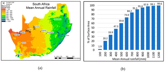
Figure 1.
(a) Map of South Africa—mean annual rainfall; (b) frequency distribution of mean annual rainfall across South Africa [30].
As shown in Figure 1b, approximately 60% of the country has an annual rainfall of less than 500 mm [31], while Figure 1a clearly shows that only small clusters of the country receive more than 1000 mm per year. This uneven distribution highlights the challenges with quantifying water availability across uneven distributions in arid regions.
2.1. Water Availability in South Africa
In this study, water availability reflects the amount of water that is readily available for abstraction at the rates required for the operation of a CSP plant at full capacity. Three core principles need to be considered when quantifying water availability: the geographic or spatial scale, the temporal scale, and the resource type. With regards to the geographic scale, for the purposes of hydrological analysis, the watersheds in South Africa are divided into primary, secondary, tertiary, and quaternary catchments [32]. These 1946 delineated boundaries represent the most detailed level of operational catchment management and planning by the Department of Water and Sanitation (DWS) in South Africa and are therefore used as the spatial scale of choice. Secondly, water resources fluctuate seasonally in most regions, following rainfall patterns, and thus the use of annual volumes does not capture the actual minimum available volume available throughout a calendar year. For this reason, monthly available volumes are used to define water availability in this study. Finally, in terms of the resource type, only surface water in national dams and perennial rivers, as well as ground water in aquifers, is considered a viable source for CSP in this work.
The seasonal variability of these three types of water resources can typically be determined in two ways—hydrological modelling, such as the Pitman model for South Africa [33,34], or statistical analysis of historical hydrological records [35]. The use of long-term hydrological records was chosen. The custodian of hydrological data in South Africa is the DWS, as established in the National Water Act of 1998 [36]. Information logged by DWS is publicly available through hydrological officers who process requests and issue the relevant information.
The primary (lowest–level detail) and quaternary (highest–level detail) catchments are shown in Figure 2, along with the quaternary catchments (QCs) where CSP is likely to be developed, indicating the study region.
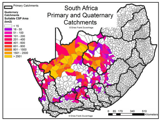
Figure 2.
Map of South Africa—primary and quaternary catchments [32].
This approach used large amounts of historical hydrological data kept by the DWS for river flows and dam storage levels in South Africa. The data is gathered in near real time and is stored on the DWS’s HYDSTRA database for public access. HYDSTRA is the name given to the South African Department of Water and Sanitation’s hydrological records database management system. The advantage of this method is that through using the actual monitored flows and dam storage volumes, the actual responses of the hydrological system to the entire water balance in a certain region are captured. This means that all inputs and abstractions into the water balance are already accounted for when the historical data for a dam or river is analysed. Neither the individual withdrawal rates of upstream processes, nor the rainfall inputs of upstream catchments are required to determine the amount of water readily available for abstraction at a certain location, because their final impact on the system is already reflected.
2.1.1. Hydrological Data in South Africa
Rivers
Figure 3 shows the rivers and flow-monitoring points for South Africa in the study region. The river dataset is publicly available from the DWS website. As can be seen from the River Class symbology used, there are very few perennial rivers in the study region, also reflected by the limited amount of monitoring points along rivers there. In order to determine the quantity of water available for abstraction from a river within a particular QC boundary, the monthly flow volumes recorded at the monitoring points along that river were analysed. The historical period with available data varied for each monitoring point based on the date they were commissioned by the DWS and the maintenance of the station. The data used represents the total volume of water that flowed past that monitoring point during the month in question in million cubic meters (Mm3). Data periods from available records range between 1 and 108 years, dating as far back as January 1904. The available data for each monitoring point within the primary catchment areas (thick grey boundaries) where CSP development is likely to take place was analysed for each month. A total of 261 monitoring points, representing 111 individual rivers, were analysed.
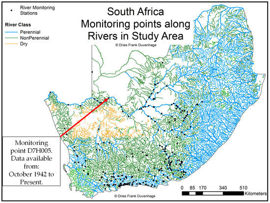
Figure 3.
Map of South Africa—rivers and river data monitoring points within the study region (data available online at http://www.dwa.gov.za/iwqs/gis_data/).
The monthly average, 90th and 10th percentile values were calculated for the period of available data for each monitoring point. The 90th and 10th percentile values represent the total volumes that are exceeded 10% (90th—floods) and 90% (10th—firm yield) of the time, respectively. A sample of this data (black lines) and its calculated average (double blue lines), 90th (red striped) and 10th percentile values (yellow dashed) are shown for monitoring point D7H005 on the Orange River, in Figure 4 for the period January 2000 to December 2017. A logarithmic scale is used in order to effectively compare the actual monthly volumes to the 90th (low exceedance probability) and 10th (high exceedance probability) percentile values. The 10th percentile was then halved, in line with the approach used in [37], in order to account for the ecological reserve requirements in that river. This value represents a very conservative quantification of water readily available for abstraction from the river section along which that monitoring point is located.
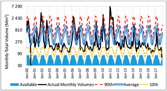
Figure 4.
Graph of actual, average, 90th, and 10th percentile monthly river flow volumes for the Orange River at D7H005.
After applying the above statistical method to quantify water availability to all rivers with monitoring points in the study region, an approach was required to aggregate the values from all monitoring points along river sections and ultimately to the QCs in which they are found. There are different cases for monitoring point placement within each QC—there could be multiple monitoring points, one, or none along the same river. Figure 5 shows these cases along the major river in the study region, the Orange River. The QCs have now been colour graded according to the total annual flow volume. In cases with only one monitoring point within a QC, that point was used to calculate the available water from the particular river and QC.
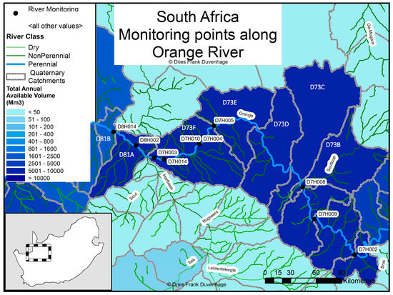
Figure 5.
Map of South Africa—monitoring points along Orange River in the study region (data available online at http://www.dwa.gov.za/iwqs/gis_data/).
In cases with no monitoring points within a QC, data from the next upstream QC with data along that river was used. No losses are accounted for from one QC to another in this case, since these would have to be based on assumptions with no real-world reference. In the case of D73D and D73C, in Figure 5, there are no monitoring points located in each of them. The next upstream QC with a monitoring point is D73B, with a data record period of 85 years. Therefore, the total annual available water of 6947 Mm3 from D73B was used for D73D and D73C. This method has limitations, since it does not account for any abstractions or runoff within D73D and D73C themselves. However, considering that the total annual available water for the next QC with its own monitoring point, D73E, has a total annual available volume of 6689 Mm3, which is lower than the upstream volumes, it at least follows the general logic of a hydrological mass balance along the river in question.
In cases with multiple points along the same river within a QC, such as for D73F (D7H004, D7H010, D7H014 and D7H003), the data had to be aggregated in such a way so as to represent available water from the river as accurately as possible, without replacing data from one point with that of another. Furthermore, some of the points would have data for certain periods, while others would not, and certain points would have data for longer periods than others. Data was aggregated and combined in these cases according to different criteria based on a hierarchal approach. The criteria used to select data points and their data was data record period length and relative position within the QC, i.e., how far downstream the point is. The rationale is that the most downstream point would be the most representative of how much water is available for abstraction within that particular QC. However, if the data record period of the more downstream point is too short, it will not provide an effective indication of long-term available water. If there were gaps in the most downstream dataset, they would be filled with the data of the next upstream point with the longest record period. In this manner, data would be combined to create a congruent, non-conflicting data record for that particular QC.
Dams
Similarly, the dams across South Africa that are under the administration of the DWS were considered as potential sources for abstraction. The DWS also keeps data for dams, with records for approximately 215 dams dating back to February 1900. These records are typically stored as water level readings in meters above sea level (MASL). However, these records alone do not provide a quantifiable indication of what volume of water is stored. Therefore, each dam has a calibrated calculation of the relationship between the MASL readings and volume, and this data can be requested from the DWS’s HYDSTRA database (available at http://www.dwa.gov.za/Hydrology/default.aspx, or per request from a hydrology officer). Monthly average volume in Mm3 was used to align with data obtained for total monthly river flow volumes. The dams for which records were obtained are shown in Figure 6.
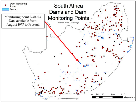
Figure 6.
Map of South Africa—dams and dam monitoring points (data available online at http://www.dwa.gov.za/iwqs/gis_data/).
Since dams do not represent a flow of water, if there are multiple dams in a QC, their combined volume can simply be calculated by adding them to each other for that month. The same statistical approach was used as for rivers, where the acquired records of monthly storage volumes were used to calculate monthly average, 90th and 10th percentile values. A sample of this data is shown for the Vanderkloof Dam, and its monitoring point D3R003 for the period January 2000 to December 2017 in Figure 7.
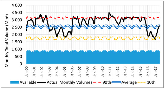
Figure 7.
Graph of actual, average, 90th, and 10th percentile monthly dam storage volumes for Vanderkloof Dam at D3R003.
The same conservative approach used for rivers was applied to the dams, where half of the monthly 10th percentile values, calculated for the entire record period for each monitoring point, were used to represent available water. This approach makes provision for existing water withdrawals from the dam, as well as the minimum storage required to supply the ecological reserve requirements to downstream rivers.
Ground Water
These resources have served as affordable, and often high-quality, water sources for development in arid regions, and have become stressed in many regions as a result [38]. The quantification of the usable volume from subterranean aquifers is a difficult task, and typically the safe reliable yield of an aquifer needs to be determined at that specific location based on pump tests [39]. However, detailed studies have been performed to quantify ground water availability at the national level, with a detailed review of the past Groundwater Resource Assessments (GRAs) for South Africa presented in [40]. These GRAs provide estimations of aquifer storage volumes, recharge rates, and yield. These estimations are based on a combination of borehole-level measurement records and hydrogeological modelling, and take into account various technical interactions between geology, soil permeability, runoff, and withdrawals [41]. The database of available groundwater, on the DWS’s National Integrated Water Information System, was used, which provides groundwater balances in Mm3/year per QC, as shown in Figure 8.
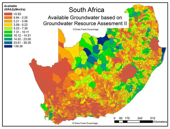
Figure 8.
Map of South Africa—available groundwater in Mm3 (data available online at http://niwis.dws.gov.za/).
These annual values for groundwater availability were simply divided by 12 to provide a monthly estimation of availability. Naturally, this approach is limited in its sensitivity to seasonal variations. However, considering the limited availability of up-to-date data on subannual groundwater resource balances, this approach at least prevents the exceedance of annual volumes.
2.1.2. Aggregated Water Balance
The data for these three water resources was aggregated per QC to determine the total available water balance by simply adding the respective monthly volumes together, per QC. The process described in Section 2.1.1 for rivers explains what approach was used to prevent double counting different flow-monitoring points along the same river network within a QC. Dams can be summed explicitly. Groundwater is reported for the entire QC, and therefore needs no special spatial considerations. The final aggregate available water balances in Mm3 (or GL) for the study region within South Africa, for January (summer), April (autumn), July (winter) and October (spring), are shown in Figure 9.
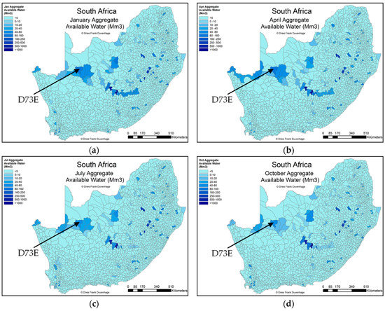
Figure 9.
Maps of South Africa—monthly aggregate available water for (a) January, (b) April, (c) July and (d) October.
As can be seen, when compared to the locations of dams in Figure 6, the QCs with large dams have the most stable monthly water supply throughout the year. Furthermore, the aggregate available water along the Orange River remains the most stable in the arid region where CSP is likely to be developed.
2.2. Water Demand from CSP
The major driver of water consumption at a CSP plant is cooling [10]. A high-level efficiency model (HLEM) was developed to calculate water demand from CSP plants based on validated monthly efficiency calculations and assumptions [24]. The model calculates the monthly performance of Parabolic Trough (PT) and Central Receiver (CR) CSP plants, with either dry or wet cooling, at any location, as identified in [22], at a scale of 1 × 1 km. The HLEM requires the monthly input data shown in Table 1. The spatial resolution of the location—linked HLEM model is only limited by the spatial resolution of the input data. However, all input data from Table 1 was resampled from the original raster resolution to a scale of 1 × 1 km, as demonstrated in Figure 10 for January dry bulb temperature [42].

Table 1.
Input data required for the spatiotemporal high-level efficiency model (HLEM).
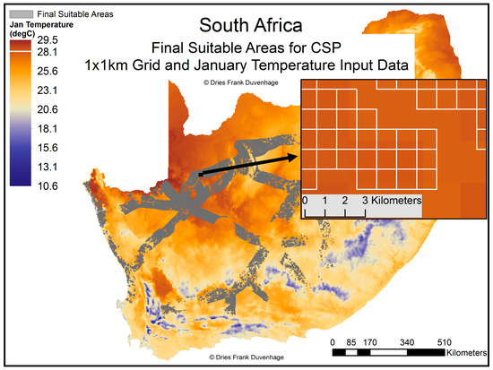
Figure 10.
Map of South Africa showing the GIS resampling process from raster to grid of the input data for the location-linked model.
The resampling process involved taking the centroid of each square and applying the input data of the raster grid, which intersects with it. This process was repeated for each month (12) of the three (3) datasets, resulting in the location-linked HLEM model capturing a total of 36 input parameters per square. Each 1 × 1 km square, therefore, represents one cell where a solar field, and likewise the heat input of a CSP-cooling configuration, was modelled.
The attribute table of this location-linked model and resampled input data was then processed in Microsoft Excel®, where the HLEM calculations were used to calculate monthly solar-to-electric efficiencies (%), the net generation potential (GWh), the water consumption factor (m3/MWh), and the total water consumption volume (m3), as described in detail in [24]. The results, calculated at the 1 × 1 km scale, were then aggregated to the QC level to determine the total monthly potential water withdrawal from the different CSP-cooling configurations inside each QC.
2.3. Linking CSP Water Demand to Water Availability
Now that both water availability and water demand from CSP can be quantified at the same spatial level, it is possible to reconcile the two and determine what amount of CSP generation can be supported by the available water resources in each QC. Naturally, because rivers are one of the types of water sources under consideration, the transfer of water between QCs, and the impact of CSP-related abstractions on downstream catchments, must also be accounted for. A systematic approach was applied, where only the water sources within each QC were first used to determine the amount of CSP that can be supported in each QC individually, without consideration for the downstream impact of this consumption. This was followed by a stream-linked approach, where the impact of this consumption in each QC was considered in downstream QCs along the same river network. This systematic approach allowed for a simple and effective way to estimate the total CSP generation potential that can be supported by the combined water resources, without neglecting the linked nature of QCs through rivers.
2.3.1. Isolated Approach—Individual Catchments
One of the key principles of this work is that the limiting factor on CSP development is not due to annual water availability, but rather subannual minima. This is because although a certain total annual volume of water is available in a certain area throughout the course of a year, this total annual volume is unequally distributed throughout that year. As such, the aggregated water balances per QC were analysed per month, as discussed in Section 2.1.
To illustrate the process used to quantify the hydrological limit on CSP development, the example of QC D73E from Figure 5 is considered. This QC (D73E) has a relatively stable monthly aggregated available water balance, as highlighted in Figure 9 and is shown in detail in Figure 11 as the blue line. The 90th percentile values represent the sum of the monthly 90th percentile values for rivers, dams and groundwater, as discussed in Section 2.1.1. The same applies to the monthly averages and 10th percentile values. The aggregate available water balance for D73E is therefore represented by the Available Balance (blue line), meaning that these volumes may not be exceeded in each of the months.
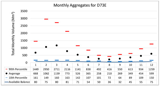
Figure 11.
Graphs of monthly aggregated balances for quaternary catchment D73E.
However, the monthly abstraction volume from CSP would depend primarily on the amount of electricity generated, and therefore, the amount of CSP developed in that QC. If the amount of CSP developed in that QC was based on the month with the greatest Available Balance (April), the demand for water would always exceed the available volume in every other month. Furthermore, if the amount of CSP developed in that QC was based on the total annual Available Balance (734 Mm3), then the monthly demand would exceed the Available Balance in some months, and not in others. It therefore follows that the actual limiting factor is the month with the lowest Available Balance, which is September, with 32 Mm3, in the example of D73E in Figure 5.
The amount of generation from a specific CSP-cooling configuration which can be supported by the water resources in a QC depends on the ratio between the monthly average consumption factor and monthly Available Balance for that QC. If the monthly Available Balance (Mm3) is divided by the monthly consumption factor (m3/MWh) for that QC, the generation potential which can be supported by that Available Balance is calculated in TWh. When this value is, in turn, divided by the monthly theoretical generation potential, based on the location–linked HLEM, then the amount of hydrologically limited CSP generation potential is expressed as a fraction thereof. This fraction is calculated for each month, and the month with the lowest fraction is used to calculate the amount of CSP generation potential for a CSP-cooling configuration in that QC. As shown in Figure 12, in the case of D73E and the Parabolic Trough Wet Cooled (PTWC) configuration, the month with the lowest hydrological limit fraction is September, at 32%. This means that only 32% of each month’s unconstrained theoretical generation potential can be supported by the aggregated water resources therein with a 90% assurance level. To illustrate this, the unconstrained theoretical generation potential and hydrologically limited CSP generation potential is shown in Figure 12, on the left axis.
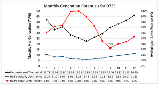
Figure 12.
Graph of monthly generation potentials and hydrological limit fractions for D73E.
The monthly total abstraction volumes for the unconstrained, and hydrologically limited cases, can now be calculated by multiplying the monthly generation potentials shown in Figure 12 with the monthly consumption factors. These monthly consumption factors are averaged across all the 1 × 1 km squares of the suitable locations within each QC. The hydrologically constrained abstraction volumes are shown in Figure 13 as the brown, dashed line, relative to the monthly 10th percentile and Available Balance aggregates for D73E. Figure 13 shows how the use of the month with the lowest hydrological limit fraction, to determine the allowed CSP generation potential, prevents the total monthly abstraction volume of this generation potential from exceeding the Available Balance in any month.
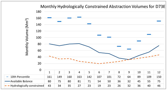
Figure 13.
Graph of monthly constrained abstraction volumes relative to the 10th percentile and Available Balance for D73E.
Based on this methodology, the hydrological limits placed on CSP generation (and therefore development) by the water resources within a certain QC are calculated, without consideration for downstream impacts. This limit is termed the isolated hydrological limit, since it ignores the relationship between QCs due to abstractions from rivers. This impact, however, cannot be ignored, and a linked catchment approach is required in order to determine the final limit on CSP development for an entire catchment and its resources.
2.3.2. Linked Catchment Approach—Downstream Catchments
The isolated hydrological limit serves as a reference point from which to determine the overall hydrological limit on CSP development. To do this, a mass balance along a primary river must be carried out, where the abstractions due to CSP development in an upstream QC are subtracted from that QC’s water balance, as well as from downstream QCs’ water balances. To perform this mass balance, however, the hydrological data used for each QC along a primary river must be temporally synchronised. If this is not the case, then hydrological data used to quantify the aggregated balance in one QC might be from a drier period, while the data used for another adjacent QC might be from a wetter period.
This is quite common for the data used across the study region, due to river-monitoring points being commissioned in different years, or due to temporary or indefinite data loss. This problem is illustrated for three monitoring points along the same river in the same QC in Figure 14, with D7H008 being the most upstream, D7H005 in the middle, and D7H004 the most downstream. As can be seen, D7H008 has the longest recording period from October 1932 to present, with a clear data loss from 2008 to 2009. D7H005 has the second longest recording period, from October 1942 to present, and a long period of overlap with D7H008. D7H004 has the shortest recording period, from August 1971 to present. It is noteworthy that the three monitoring points’ records roughly follow the same typical response curves.
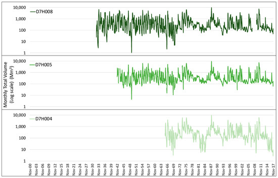
Figure 14.
Graphs of monthly total river flow volumes for three adjacent monitoring points along the Orange River.
If the period of overlap is used alone for the three monitoring points in Figure 14, data fidelity will be lost for points with longer records. As such, the full recording period of each point is used. However, to overcome the lack of temporal synchronisation required for an accurate mass balance, a relative volume reduction ratio is used to represent the links between QCs along the same primary river. This will provide a relatively simple approach to account for the reduction of water availability in downstream QCs because of CSP–related abstractions in an upstream QC. The rationale behind this approach is confirmed by the relative agreement between the three monitoring points’ monthly flow volumes in Figure 14.
Therefore, instead of subtracting the consumption of CSP development in one QC from that of downstream QC water balances, these downstream balances are proportionally reduced based on the abstraction in the upstream QC. For example, if the volume abstracted due to CSP development in the upstream QC represents 15% of that QC’s 10th percentile aggregated water balance, then the downstream QC aggregated water balances are now only 85% of their 10th percentile volumes prior to CSP development. Naturally, a critical aspect of this approach is which statistical monthly volume (10th, 90th, or average) is used as the denominator in the calculation of the relative reduction in available volume. If the monthly 10th percentile is used, the relative reduction will be larger than if the monthly average is used. The monthly 90th percentile is not considered an effective option since this represents floods, and therefore not typical flow conditions.
To ensure the approach takes into account the most common conditions, and to provide the most conservative relative reduction in available volume, the monthly 10th percentile is used as the denominator in the equation . represents the percentage volume available after CSP-related abstractions, represents the volume abstracted by CSP developments in QC only for month , and represents the original aggregated (river, dam and groundwater) monthly 10th percentile volume for QC and month , as discussed in Section 2.1.1. The aggregated balance is used since the abstractions from a section of river will ultimately reduce the total volume stored in affected QCs because rivers serve as the main transfer of water between both groundwater and dam storages within the hydrological cycle. The values of each downstream QC are then multiplied with each other in order to determine the accumulated effect of reduced aggregated water balances along the entire primary river. To calculate the balance in the QC along a primary river, the values of all QCs with stream ranks lower than (ranked from upstream to downstream, i.e., 1 to ) are multiplied with each other in order to capture the reduced balance in QC due to upstream CSP-related abstractions in QC 1 to . The abstractions calculated for QC are then finally subtracted from the remaining aggregated 10th percentile volumes.
As an example, from Figure 5, the case for D73C, D73D, D73E and D73F is shown in Table 2 for January (). This is for the scenario where all possible CSP developments, based on the isolated hydrological limit for each individual QC, can abstract water from the aggregated balance for that QC. Naturally, since the first QC for this example is ranked 38th, it has 37 other QCs upstream thereof along the primary river (the Orange River). Therefore, its cumulative value (col. 6) is already low at 10.93%, and so only 10.93% of its pre-CSP monthly 10th percentile aggregated balance is available for further abstractions because of upstream CSP-related abstractions. After the CSP-related abstraction within each QC is subtracted from its the remaining available water due to upstream abstractions, the final linked catchment balance for each QC is calculated (col. 7). The values in column 7 show that if the maximum amount of CSP based on the isolated hydrological limits of each QC is fully developed, then a hydrological deficit will be reached in downstream QCs due to reduced transfer between QCs.
Table 2.
Linked catchment calculated values for quaternary catchment (QC) D73C, D73D, D73E and D73F along the Orange River for Parabolic Trough Wet Cooled (PTWC).
Since this 100% development of CSP per QC results in certain QCs experiencing deficits, another approach was needed to prevent this. This presents two questions—which QCs are selected for CSP development, and, if they are selected, to what extent? To address this, a sequence of four scenarios were calculated based on the extent to which CSP is developed in each QC.
3. Results—Limits Imposed by Water Availability on CSP Development
Based on the methodology presented in this paper, a sequence of hydrological constraints on CSP development can be calculated for each hydrological planning area (in this case, QCs). This sequence of hydrological constraints takes the form of four scenarios: no hydrological constraints (unconstrained), constraints based on isolated QC balances (isolated), constraints based on linked catchment balances with an overall relative reduction in CSP capacity from the isolated QC approach to prevent downstream catchments from being depleted (downstream), and finally, constraints based on linked catchment balances according on an optimised relative reduction in CSP capacity according to a priority index (optimised). These four scenarios are carried out at a national scale for the four CSP-cooling technology configurations: Parabolic Trough Wet Cooled (PTWC), Central Receiver Wet Cooled (CRWC), Parabolic Trough Dry Cooled (PTDC) and Central Receiver Dry Cooled (CRDC).
The rationale behind the four hydrological constraints is to start from a worst-case unconstrained scenario, where all theoretically suitable CSP development is carried out and the impact thereof on water balances is quantified. This provides a baseline from which to calculate the hydrologically limited CSP development capacities. From this, the isolated scenario calculates CSP development capacities based on the isolated impact thereof with each respective QC, with no consideration for downstream impacts of QCs linked by a perennial river. This isolated constraint is calculated as a percentage of the unconstrained CSP generation potential, as described in Section 2.3, based on the month with the lowest relative water availability for each QC. While this scenario does address the limitations imposed by water resources on CSP development, it does not do so in a way that considers downstream impacts across an entire primary catchment.
Therefore, a linked catchment scenario is required to determine what percentage of CSP development of the isolated scenario can be supported in each QC while still maintaining a balance in downstream QCs above the reserve margin described in Section 2.1. The downstream scenario does this by reducing all monthly CSP generation potentials from the isolated scenarios by a flat rate across all QCs. It is carried out iteratively to ensure the minimum balance in all downstream QCs stays above the environmental reserve (half of the 10th percentile aggregated balance). Finally, the optimised scenario follows a similar method to the downstream scenario; however, instead of applying a flat relative reduction to the isolated constraints across all QCs, the QCs are ranked according to a priority index and individually optimised along each primary catchment in order to maintain the ecological reserve in each QC. This optimisation allows the QCs with the highest theoretical CSP development potential along a primary river to undergo higher rates of development.
To calculate a priority index, the theoretical annual net generation of each QC (as discussed in Section 2.2.) was divided by the total theoretically suitable area for that QC, giving the net generation potential (GWh) per square kilometre. However, in order to capture the priority rank of that QC along its primary river, this value is multiplied with the primary river area ratio, which is the total theoretically suitable area within each QC divided by the total theoretically suitable area along its entire primary river.
Table 3 provides the values for these calculations for the same QCs as in Table 2, and shown in Figure 5. As shown in column 6, QC D73C has the highest rank because, even though it has the lowest relative net annual generation potential per square kilometre, it has the most theoretically suitable area along the primary river (Orange River), and therefore it has the greatest potential for CSP development. These ranking calculations are performed for all QCs, and CSP development can now be prioritised in areas with the highest of these ranks. Since the QCs have now been ranked, the suitable areas within each QC should undergo the same process of prioritisation. However, at this stage, an indiscriminately selected percentage is only allocated per QC.
Table 3.
Priority index values calculated for QC D73C, D73D, D73E and D73F along the Orange River.
What this means is that now the QCs with the highest rank can be allocated the largest development share, relative to the isolated scenario. For example, for the PTWC CSP-cooling configuration, D73C can be allocated 47%, D73D 11%, D73E 15% and D73F 23% of their respective 100% isolated hydrological limit for CSP development for that CSP-cooling configuration. These allocations were calculated iteratively, in a similar manner to that of the downstream scenario. They can be varied depending on what the user wants to optimise for: cost of electricity production—then the suitable areas with highest DNI and which are the nearest to water sources must be given priority; economic development in desired municipal areas—then these can be identified and the QCs within their boundaries can be given priority; minimised flow reduction in low runoff catchments—then the more upstream QCs, with higher self-generated runoff values can receive priority for CSP development, and so on.
This prioritisation, however, is still somewhat arbitrary, since the development of CSP in one location, and therefore one QC, instead of another, ultimately depends greatly on the amount and type of government regulation dictating this decision by independent developers. Therefore, the following calculations of linked catchment hydrological limits should serve only as an initial indication of what the hydrologically sustainable development potential for CSP is in each QC. These limits should ultimately be updated as part of an interdepartmental adaptive management strategy for water resources and CSP between the Department of Energy (DoE) and DWS of South Africa. Part of this strategy should be the addition of new data on hydrological records and proposed CSP plants into the models to ensure that the most recent hydrological changes and CSP developments are considered. The results from these hydrological constraint scenarios and CSP-cooling configurations will now be discussed.
3.1. Parabolic Trough Wet Cooled (PTWC) and Central Receiver Wet Cooled (CRWC)
The 50 MW PTWC CSP-cooling configuration, which was modelled in the location-linked HLEM, serves as a realistic indication of water consumption at PTWC plants in South Africa. The 100 MW configuration was also modelled, with the primary difference in results being a slightly higher turbine efficiency, translating to a higher solar-to-electric (StE) efficiency. While the 100 MW configuration does have proportionately lower water consumption rates due to the higher efficiencies, the results were not included in this work since the 50 MW case serves as a worst-case point of reference. Despite the marginal improvements in water consumption between the 50 and 100 MW configuration, these improvements are still small in comparison to the relative difference in consumption rates between wet and dry cooling.
For CR plants, however, the increase in steam turbine efficiency from 50 to 100 MW installed capacities is countered to a great extent by the reduction in solar field efficiency due to the larger distance from heliostats to the Central Receiver on the tower. Despite this, the higher operating temperatures of CR plants with molten salt as the heat transfer fluid (HTF) mean that the steam turbine efficiencies are higher than PT plants, resulting in less heat needing to be rejected through cooling, and more heat being converted to electricity. This, in turn, results in CRWC plants with lower consumption factors, and higher StE efficiencies than PTWC plants, as shown in Figure 15 [24]. Figure 15 shows the average StE efficiencies and consumption factors across all locations modelled within the study region inside South Africa, reflecting the typical operation characteristics of these two configurations.
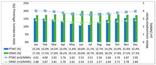
Figure 15.
National average monthly solar-to-electric efficiencies and water consumption factors for Parabolic Trough Wet Cooled (PTWC) and Central Receiver Wet Cooled (CRWC) plants.
Figure 16a,b show the national annual abstraction and generation limits for the PTWC and CRWC configurations, respectively, for the four hydrological constraint scenarios. The graphs use logarithmic scales on the y-axes due to the substantial difference in the order of magnitude between the four scenarios. The optimised scenario results in higher abstraction limits reached for both the PTWC and CRWC configurations because of the aim of the optimisation approach, namely to maximise the allocation of CSP development to QCs with higher CSP potential, resulting in better use of the available water in those QCs. This increase in both abstraction and generation limit, however, is marginal, at 12% and 15% for PTWC and CRWC, respectively.
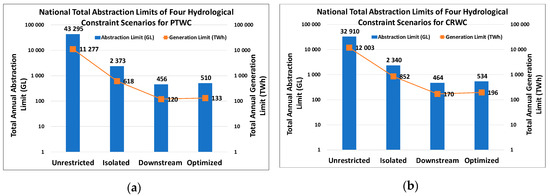
Figure 16.
Total annual abstraction limit and generation limit for South Africa for: (a) PTWC and (b) CRWC.
The spatial results for the month of July (winter), from the sequential hydrological constraint scenarios for the PTWC and CRWC configurations, are shown in Figure 17 and Figure 18, respectively. The columns refer to the hydrological constraint scenario, while the rows give different sets of results—abstraction limit in gigalitres (Mm3) and the generation limits (TWh) associated with these abstraction limits for the CSP-cooling configuration.
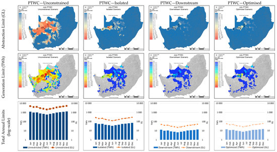
Figure 17.
Abstraction and generation limit results for hydrological constraint scenarios for July (winter) for PTWC.
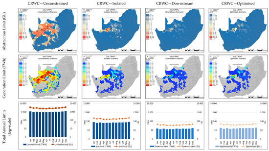
Figure 18.
Abstraction and generation limit results for hydrological constraint scenarios for July (winter) for CRWC.
Figure 17 and Figure 18 clearly show the decrease in allowable abstraction and therefore generation potential across the study area in South Africa, from the unrestricted scenario (no hydrological limits placed on CSP potential) to the isolated scenario. Where the unrestricted scenario shows the theoretical potential for PTWC and CRWC across South Africa per QC, the isolated scenario takes into consideration the limit imposed by water resource availability in each QC on this development. The downstream and optimised scenarios both show a great reduction in abstraction and generation limits from the isolated scenarios. This is because the downstream and optimised scenarios take into consideration the linked nature of QCs through perennial rivers, where abstractions in one QC are carried over to downstream QCs to reflect the total primary catchment impact of CSP-related abstractions, and the resulting limit on potential development.
When comparing Figure 16, Figure 17 and Figure 18, the impact of the higher turbine efficiency of CRWC plants and the resulting reduced consumption factor are clearly shown in the higher generation limits achievable at lower abstraction limits. The decrease in annual national generation potential for South Africa, due to the limits imposed by water availability, is from 11,277 to 133 TWh for PTWC and from 12,003 to 196 TWh for CRWC. It must be noted that these generation potentials do not consider a specific capacity factor (CF). The assumption is that every unit of solar energy is converted into electrical energy based on a StE efficiency from the location—linked HLEM, and therefore serves as the maximum theoretical electricity generation potential. If a desired CF is specified, then the required installed capacity in GW can easily be determined; and with more detailed calculations, the required hours of Thermal Energy Storage can also be established. What is clear, however, is that the hydrological limits placed on CSP development for the wet-cooled PT and CR configurations result in the hydrologically sustainable generation limit being just under 84-fold (PTWC) and just over 61-fold (CRWC) less than the theoretical generation potential.
3.2. Parabolic Trough Dry Cooled (PTDC) and Central Receiver Dry Cooled (CRDC)
Dry cooling plants in general have lower steam turbine efficiencies due to the reliance on higher ambient dry bulb temperatures for heat rejection. This, in turn, contributes toward an overall decrease in StE efficiency at both PT and CR plants compared to wet-cooled plants. Dry cooled plants, however, have no water requirements for heat rejection, meaning that the consumption patterns are less dependent on seasonal changes in ambient conditions. This ultimately results in the water consumption of dry cooled CSP plants remaining mostly constant throughout the year. Based on data obtained from a PTDC plant in South Africa, a conservative, constant water consumption factor of 0.56 m3/MWh was assumed for all DC plants. While value obtained is higher than values (0.1–0.3 m3/MWh) reported in the literature [26,45,46], it is still an order of magnitude lower than that of the wet cooling results shown in Figure 15. It is therefore a worst-case estimation of consumption at DC plants in South Africa, but maintains the relative improvement in consumption compared to wet-cooled plants. The national average monthly StE efficiencies and constant consumption factors for PTDC and CRDC plants are shown in Figure 19.
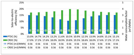
Figure 19.
National average monthly solar-to-electric efficiencies and water consumption factors for PTDC and CRDC plants.
Figure 20a,b show the national annual abstraction and generation limits for the PTDC and CRDC configurations, respectively, for the four hydrological constraint scenarios. The graphs use the same logarithmic scales on the y-axes as those in Figure 16 for comparative purposes. The optimised scenario results in higher abstraction limits reached for both the PTDC and CRDC configurations since the aim of the approach is to maximise the allocation of CSP development to QCs with higher CSP potential, resulting in better use of the available water in those QCs. This increase in both abstraction and generation limit is more substantial than for WC plants—29% for both PTWC and CRWC, respectively.
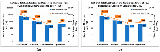
Figure 20.
Total annual abstraction and generation limit for South Africa for: (a) PTDC and (b) CRDC.
The spatial results for the month of July (winter), from the sequential hydrological constraint scenarios for the PTDC and CRDC configurations, are shown in Figure 21 and Figure 22, respectively.
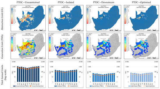
Figure 21.
Abstraction and generation limit results for hydrological constraint scenarios for July (winter) for PTDC.
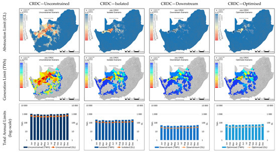
Figure 22.
Abstraction and generation limit results for hydrological constraint scenarios for July (winter) for CRDC.
Figure 20, Figure 21 and Figure 22 clearly show the decrease in allowable abstraction and therefore generation potential across the study area in South Africa, from the unrestricted scenario to the isolated scenario. What is notable, however, is that it is less drastic compared to the results for the WC plants. Due to the higher efficiencies of WC plants, they have higher national generation limits under the unconstrained scenarios than DC plants. However, for the isolated hydrological constraint scenarios, the limits achievable for DC plants are higher than those by WC plants. This is not surprising, since WC plants will exhaust water resources much quicker than DC plants and are therefore limited at lower generation limits.
Due to the limits imposed by water availability, the decrease in annual national generation potential for South Africa is from 11,038 to 371 TWh for PTDC, and from 11,824 to 409 TWh for CRDC. The hydrological limits placed on CSP development for the dry cooled PT and CR configurations result in a hydrologically sustainable generation limit just under 30-fold (PTDC) and 29-fold (CRDC) less than the theoretical, unconstrained generation potential. This means that the optimized generation limits for PTDC plants are 2.8 times greater than for PTWC plants; and that the optimized generation limits for CRDC plants are 2.1 times greater than those for CRWC plants. When comparing Figure 17 and Figure 21, and Figure 18 and Figure 22, it is clear that the generation limits are higher across all QCs for PTDC than for PTWC.
4. Discussion and Conclusions—Policy Guidelines for Sustainable CSP Development
Currently, any prospective water user in South Africa must apply for a water use license (WUL), in accordance with the National Water Act (NWA) of South Africa [36]. The NWA, however, does make special mention of two key strategic use cases—intercatchment transfers and power generation. In light of the recognition of power generation as critical to achieving improved access to electricity, set out in the National Development Plan (NDP), it is important to recognise that the achievement of this goal must not come at the cost of another NDP goal, namely improved access to water [47]. The importance of this trade off has been recognised by the DWS in a 2015 DWS guidance note on water use by coal independent power producers (IPPs) [48]. This guidance note provides a brief context on water availability across South Africa and places particular focus on the areas where coal fields are located, and therefore where coal IPPs are likely to bid to build plants. It emphasizes that water resources in general are stressed, and that bidders who implement water-saving technologies and strategies are likely to receive preference during the WUL application process.
As part of the WUL process, such as application undertaken for a CSP plant in 2010 [49], typically the applicant must perform an integrated assessment of the water availability situation in the QC where it intends to construct the plant. Water availability from the nearby water sources is assessed on an annual basis, and no consideration for the constraint, which the minimum available monthly volume places on generation and associated abstraction, is given. As part of the WUL process, however, the DWS will review the application and supporting documentation and assess water availability in the area itself, and then approve or decline the WUL.
In South Africa, there are six operational CSP plants, each with already successfully applied for WULs in order for them to be operational. The annual amounts allocated to all commercial, agricultural and industrial water users are publicly available from the Water Authorisations Office (WARMS) upon request. The water authorisations allocated to the six CSP plants were requested from DWS, and are shown in Table 4 for five of the six, with Kathu Solar Park having to apply for water use authorisation from a regional water board, because it abstracts water from a bulk water supply pipeline. These locations are also shown in the maps included in Figure 16.
Table 4.
Information for water use authorisations for existing CSP plants in South Africa and the HLEM-estimated abstraction values, the Water Authorisations Office (WARMS).
Table 4 also shows the estimated total annual abstraction volumes, based on the locations of these CSP plants, their CSP-cooling configuration, and the results from the location-linked HLEM. It is clear that the values allocated by the WARMS office to the DC plants are between 56% and 215% higher than the annual abstraction volumes estimated by the HLEM. This suggests that the DC CSP plants in SA have an overallocation of water, technically allowing them to use much more than the plant should be using. This means that the plant could be wasting water, or using it ineffectively, and the DWS will not raise any alarm because it is still below the registered volumes. The WC CSP plant, however, has a registered volume much closer to the volume estimated by the location-linked HLEM. This suggests that the WC CSP plant might be operating close to its WARMS-registered volume, placing it at risk of exceeding its allowance and being subject to penalties.
These observations demonstrate the need for more informed WUL allocations by the DWS’s WARMS office, based on better knowledge of the typical performance of the various CSP-cooling configurations in a particular location. Beyond an improved approach to quantifying suitable allocations for CSP plants, the WUL process also requires a detailed inventory of existing registered users in each QC, accompanied by an inventory of water balances per QC. This will allow the DWS to assess future water use applications, be it CSP or other water use categories, in greater detail. This will improve the sustainable allocation of water to a specific applicant on grounds of this inventory. This inventory should, however be updated continuously as new hydrological data becomes available, and as new applicants are allocated water use rights.
For CSP, as part of future IPP bidding rounds, the methodology presented in this work, with its accompanying models, can be used to guide the development of CSP in certain QCs based on the amount of water already allocated to CSP plants in those QCs. This should also take the form of an inventory of CSP water allocations, and volumes still available for future developments. Like the 2015 Guidance Note for coal IPPs, a guidance note can be generated for CSP in the areas identified in this study where CSP plants are most likely to be developed. The models used in this methodology are adaptable to accommodate the potential impact of water-saving technologies on the four CSP-cooling configurations considered. These impacts can be quantified and incorporated into the models, and the increase in hydrologically sustainable CSP development potential can be determined. Furthermore, once these potential reductions in CSP-related water consumption are determined and incorporated into the models, the DWS can suggest the use of certain technologies in order to ensure sustainable water use by CSP plants, with cognisance of the potential impact on plant operation.
This work therefore provides a set of models that can enable the custodians of water and energy planning in arid regions to better plan for CSP development and ensure hydrological sustainability. It was found that the hydrological limits in South Africa drastically reduce the amount of CSP that can be developed relative to the theoretical, unconstrained potential. This reduction is much greater for water-intensive wet-cooled plants, with the downstream hydrological CSP generation potential being only 1.06% and 1.42% of the theoretical unconstrained generation potential for PTWC and CRWC, respectively. The much less water-intensive dry cooled CSP plants also experience hydrological limits, albeit much lower than that of wet-cooled plants, with the downstream hydrological constraints being 4.64% and 6.18% of the theoretical unconstrained generation potential for PTDC and CRDC plants, respectively.
To guide energy policy makers, this work shows that the use of dry cooled plants can allow for greater exploitation of the greater economic benefits associated with CSP above other renewable technologies [50]. Since CSP is comprised of many subsystems of technologies for which there are mature technical capabilities and skills in South Africa, the use of dry cooled CSP plants will allow for more hydrologically sustainable CSP, and therefore contribute more to the stimulation of these associated industries. Furthermore, the models and tools presented in this work can be used to assess the hydrological impact of CSP developments in areas of economic interest. This can, in turn, further motivate the development of CSP in South Africa, without placing water resources under unsustainable stress. The methods used in this work are not exhaustive, and improvements can be made in the spatiotemporal modelling of dry cooled plants in particular, as well as in the hydrological quantification of water availability. The intention of this work, however, is to present an initial high-level strategic assessment of CSP development and water resources in arid regions, and specifically South Africa. This study provides a detailed account of the methodology used to determine the first documented investigation of the hydrological limits placed on CSP development.
Author Contributions
Conceptualisation, D.F.D.; formal analysis, D.F.D.; methodology, D.F.D.; supervision, A.C.B., W.H.L.S., and S.G.; validation, D.F.D.; writing—original draft, D.F.D.; writing—review and editing, A.C.B. All authors have read and agreed to the published version of the manuscript.
Funding
Part of this work was funded by the National Research Foundation of South Africa. Work carried out on the ColSim CSP simulation suite was funded by the European Union’s Horizon 2020 research and innovation programme, under grant agreement no. 654443 (MinwaterCSP).
Acknowledgments
This work forms part of the research of Frank Duvenhage and, as such, is made possible by Stellenbosch University’s Department of Industrial Engineering and the Solar Thermal Energy Research Group. Thanks go to Alan Brent for his continuous support, Fraunhofer ISE for support with CSP simulations, the hydrological officers at the DWS (in particular Boshomane) for hydrological data, van der Heever from Legal Drone Solutions for support with GIS, the CM SAF operation team for detailed monthly DNI data, and the management team at Bokpoort CSP plant and SolarPACES.
Conflicts of Interest
The authors declare no conflict of interest.
Abbreviations
| CF | Capacity Factor |
| CSP | Concentrating Solar Power |
| CR | Central Receiver |
| CRDC | Central Receiver Dry Cooled |
| CRWC | Central Receiver Wet Cooled |
| DC | Dry Cooled |
| DHIS | Detailed Hourly Interval Simulation |
| DNI | Direct Normal Irradiance |
| DoE | Department of Energy (RSA) |
| DWS | Department of Water and Sanitation (RSA) |
| GIS | Geographic Information Systems |
| GL | Gigalitre (same as Mm3—1,000,000,000 litres) |
| GRA | Groundwater Resource Assessment |
| GWh | Giga Watt-Hours |
| HLEM | High-Level Efficiency Model |
| HTF | The Heat Transfer Fluid |
| IRP | Integrated Resource Plan |
| LCOE | Levelized Cost of Electricity |
| MASL | Meters Above Sea Level |
| Mm3 | Million Cubic Meters |
| MWh | Mega Watt-Hours |
| NWA | National Water Act |
| PT | Parabolic Trough |
| PTDC | Parabolic Trough Dry Cooled |
| PTWC | Parabolic Trough Wet Cooled |
| QC | Quaternary Catchment |
| RET | Renewable Energy Technology |
| StE | Solar-to-Electric |
| TES | Thermal Energy Storage |
| TWh | Terra Watt-Hour |
| VRE | Variable Renewable Energy |
| WARMS | Water Authorisations Office (DWS of RSA) |
| WC | Wet Cooled |
| WEF | Water–Energy–Food |
| WUL | Water Use License |
References
- Albrecht, T.R.; Crootof, A.; Scott, C.A. The Water-Energy-Food Nexus: A Systematic Review of Methods for Nexus Assessment. Environ. Res. Lett. 2018, 13. [Google Scholar] [CrossRef]
- Bizikova, L.; Roy, D.; Swanson, D.; Venema, D.H.; Mccandless, M. The Water–Energy–Food Security Nexus: Towards A Practical Planning And Decision-Support Framework For Landscape Investment And Risk Management; International Institute for Sustainable Development: Winnipeg, MB, Canada, 2013. [Google Scholar]
- Endo, A.; Tsurita, I.; Burnett, K.; Orencio, P.M. A Review of the Current State of Research on the Water, Energy, and Food Nexus. J. Hydrol. Reg. Stud. 2017, 11, 20–30. [Google Scholar] [CrossRef]
- Liu, J.; Hull, V.; Godfray, H.C.J.; Tilman, D.; Gleick, P.; Hoff, H.; Pahl-Wostl, C.; Xu, Z.; Chung, M.G.; Sun, J.; et al. Nexus Approaches to Global Sustainable Development. Nat. Sustain. 2018. [Google Scholar] [CrossRef]
- Simpson, G.B.; Jewitt, G.P.W.; Simpson, G.B. The Development of The Water-Energy-Food Nexus as a Framework for Achieving Resource Security: A Review. Front. Environ. Sci. 2019, 7, 1–9. [Google Scholar] [CrossRef]
- Weitz, N.; Strambo, C.; Kemp-Benedict, E.; Nilsson, M. Closing The Governance Gaps in the Water-Energy-Food Nexus: Insights from Integrative Governance. Glob. Environ. Chang. 2017, 45, 165–173. [Google Scholar] [CrossRef]
- Mabrey, D.; Vittorio, M. Moving From Theory To Practice In The Water–Energy–Food Nexus: An Evaluation of Existing Models And Frameworks. Water-Energy Nexus 2018, 1, 17–25. [Google Scholar]
- Gauché, P.; Pfenninger, S.; Meyer, A.J.; Von Backström, T.W.; Brent, A.C. Modeling Dispatchability Potential of CSP In South Africa. In Proceedings of the Southern African Solar Energy Conference (SASEC), Stellenbosch, South Africa, 21–23 May 2012; Volume 1, pp. 1–11. [Google Scholar]
- Gauché, P.; Von Backström, T.W.; Brent, A.C. A Concentrating Solar Power Value Proposition for South Africa. J. Energy S. Afr. 2013, 24, 67–76. [Google Scholar] [CrossRef][Green Version]
- Duvenhage, D.F.; Brent, A.C.; Stafford, W.H.L. The Need to Strategically Manage CSP Fleet Development and Water Resources: A Structured Review and Way Forward. Renew. Energy 2019, 132, 813–825. [Google Scholar] [CrossRef]
- Ali, B. Forecasting Model For Water-Energy Nexus In Alberta, Canada Canadian Association of Petroleum Producers The United States of America. Water-Energy Nexus 2018, 1, 104–115. [Google Scholar] [CrossRef]
- Pouris, A.; Thiopil, G.A. Long Term Forecasts Of Water Usage For Electricity Generation: South Africa 2030. Report No. 2383/1/14; Water Research Commission: Lynnwood Manor, South Africa, 2015. [Google Scholar]
- Liu, L.; Hejazi, M.; Patel, P.; Kyle, P.; Davies, E.; Zhou, Y.; Clarke, L.; Edmonds, J. Water Demands for Electricity Generation in the U.S.: Modeling Different Scenarios For The Water-Energy Nexus. Technol. Forecast. Soc. Change 2015, 94, 318–334. [Google Scholar] [CrossRef]
- Davies, E.G.R.; Kyle, P.; Edmonds, J.A. Advances In Water Resources An Integrated Assessment of Global And Regional Water Demands For Electricity Generation To 2095. Adv. Water Resour. 2013, 52, 296–313. [Google Scholar] [CrossRef]
- Khan, Z.; Linares, P.; García-González, J. Integrating Water And Energy Models For Policy Driven Applications. A Review of Contemporary Work And Recommendations For Future Developments. Renew. Sustain. Energy Rev. 2017, 67, 1123–1138. [Google Scholar] [CrossRef]
- DWS. Strategic Overview Of The Water Sector In South Africa 2015; Department Water And Sanitation: Pretoria, South Africa, 2015.
- IPP Office. Independent Power Producers Procurement Programme An Overview December 2018; RSA: Pretoria, South Africa, 2018. [Google Scholar]
- Duvenhage, D.F.; Craig, O.O.; Brent, A.C.; Stafford, W.H.L. Future CSP In South Africa—A Review of Generation Mix Models, Their Assumptions, Methods, Results And Implications. In Proceedings of the AIP Conference, Maharashtra, India, 5–6 July 2018; Volume 2033, p. 120002. [Google Scholar]
- Silinga, C.; Gauché, P.; Van Niekerk, W. CSP Scenarios In South Africa: Benefits of CSP and the Lessons Learned. In Proceedings of the Solarpaces Conference 2015, Cape Town, South Africa, 13–16 October 2015; Volume 070031, pp. 1–8. [Google Scholar]
- Pollet, B.G.; Staffell, I.; Adamson, K.-A. Current Energy Landscape In The Republic of South Africa. Int. J. Hydrogen Energy 2015, 40, 16685–16701. [Google Scholar] [CrossRef]
- ERC; CSIR; IFPRI. The Developing Energy Landscape In South Africa: Technical Report; Energy Research Centre, University of Cape Town: Cape Town, South Africa, 2017. [Google Scholar]
- Duvenhage, D.F.; Brent, A.C.; Stafford, W.; Van Den Heever, D. Concentrating Solar Power Potential in South Africa—An Updated GIS Analysis. Int. J. Smart Grid Clean Energy 2019. in preprint. [Google Scholar]
- Duvenhage, D.F.; Brent, A.C.; Stafford, W.H.L.; Craig, O.O. Water And CSP—A Preliminary Methodology for Strategic Water Demand Assessment. In Proceedings of the Solarpaces 2018—In Review; AIP Publishing: Casablanca, Morocco, 2018. [Google Scholar]
- Duvenhage, D.F. Sustainable Future CSP Fleet Deployment In South Africa: A Hydrological Approach To Strategic Management; Stellenbosch University: Stellenbosch, South Africa, 2019. [Google Scholar]
- Macknick, J.; Newmark, R.; Heath, G.; Hallett, K.C. A Review of Operational Water Consumption and Withdrawal Factors for Electricity Generating Technologies. Natl. Renew. Energy Lab. 2011, 21. [Google Scholar]
- Turchi, C.; Wagner, M.; Kutscher, C. Water Use In Parabolic Trough Power Plants: Summary Results From Worleyparsons’ Analyses; NREL: Golden, CO, USA, 2010. [Google Scholar]
- Madhlopa, A.; Keen, S.; Sparks, D.; Moorlach, M.; Dane, A. Renewable Energy Choices and Water Requirements In South Africa. Report for the Water Research Commission; Water Research Commission: Cape Town, South Africa, 2013. [Google Scholar]
- Luo, T.; Young, R.; Reig, P. Aqueduct Projected Water Stress Country Rankings. World Resour. Inst. 2015, 1–16. [Google Scholar]
- Gassert, F.; Landis, M.; Luck, M.; Reig, P.; Shiao, T. Aqueduct Global Maps 2.1: Constructing Decision-Relevant Global Water Risk Indicators; World Resources Institute: Washington, DC, USA, 2014. [Google Scholar]
- Schulze, R.E.; Lynch, S.D. Annual Precipitation. In South African Atlas Of Climatology And Agrohydrology. WRC Report 1489/1/06, Section 6.2; Schulze, R.E., Ed.; RSA: Pretoria, South Africa, 2007. [Google Scholar]
- King, J.; Pienaar, H. Sustainable Use of South Africa’s Inland Waters; Water Research Commission: Lynnwood Manor, South Africa, 2011; ISBN 978-1-4312-0129-7. [Google Scholar]
- Schulze, R.E.; Hallowes, L.A.; Horan, M.J.C.; Lumsden, T.G.; Pike, A.; Thornton-Dibb, S.; Warburton, M.L. South African Quaternary Catchments Database. In South African Atlas Of Climatology And Agrohydrology. WRC Report 1489/1/06, Section 2.3; Schulze, R.E., Ed.; RSA: Pretoria, South Africa, 2007. [Google Scholar]
- Pitman, W.V. A Mathematical Model For Generating Monthly River Flows From Meteorological Data In South Africa. HRU Report No. 2/73; Hydrological Research Unit, University Of The Witwatersrand: Johannesburg, South Africa, 1973. [Google Scholar]
- Hughes, D.A. A Review Of 40 Years Of Hydrological Science And Practice In Southern Africa Using The Pitman Rainfall-Runoff Model. J. Hydrol. 2013, 501, 111–124. [Google Scholar] [CrossRef]
- Grimaldi, S.; Kao, S.C.; Castellarin, A.; Papalexiou, S.M.; Viglione, A.; Laio, F.; Aksoy, H.; Gedikli, A. Statistical Hydrology; Elsevier: Amsterdam, The Netherlands, 2010; Volume 2, ISBN 9780444531933. [Google Scholar]
- Republic of South Africa. National Water Act. Act No 36 Of 1998; Republic of South Africa: Cape Town, South Africa, 1998; p. 94.
- Macknick, J.; Cohen, S.; Newmark, R.; Martinez, A.; Sullivan, P.; Tidwell, V. Water Constraints In An Electric Sector Capacity Expansion Model. Natl. Renew. Energy Lab. 2015. [Google Scholar]
- Zhou, Y. A Critical Review Of Groundwater Budget Myth, Safe Yield And Sustainability. J. Hydrol. 2009, 370, 207–213. [Google Scholar] [CrossRef]
- Rezaei, A.; Mohammadi, Z. Annual Safe Groundwater Yield In A Semiarid Basin Using Combination Of Water Balance Equation And Water Table Fluctuation. J. African Earth Sci. 2017, 134, 241–248. [Google Scholar] [CrossRef]
- Witthuser, K.; Cobbing, J.; Titus, R. Review Of GRA1, GRA2 And International Assessment Methodologies. P RSA 000/00/11609/6; RSA: Pretoria, South Africa, 2009. [Google Scholar]
- Woodford, A.; Rosewarne, P.; Girman, J. How Much Groundwater Does South Africa Have? In Proceedings of the 59th Canadian Geotechnical Conference, 7th Joint CGS/IAH-CNC Groundwater Specialty Conference, Vancouver, BC, Canada, 1–4 October 2006; pp. 1294–1300. [Google Scholar]
- Schulze, R.E.; Hallowes, L.A.; Horan, M.J.C.; Lumsden, T.G.; Pike, A.; Thornton-Dibb, S.; Warburton, M.L. DAILY MEAN TEMPERATURES. In South African Atlas Of Climatology And Agrohydrology. WRC Report 1489/1/06, Section 7.7; Schulze, R.E., Ed.; RSA: Pretoria, South Africa, 2007. [Google Scholar]
- Richard, M.; Uwe, P.; Christine, T.-C.; Roswitha, C.; Jörg, T.; Hollmann, R. Surface Solar Radiation Data Set-Heliosat (SARAH), 1st ed.; Satellite Application Facility On Climate Monitorin: Offenbach, Germany, 2015. [Google Scholar]
- Schulze, R.E. Preface And Executive Summary. In South African Atlas Of Climatology And Agrohydrology. WRC Report 1489/1/06; Schulze, R.E., Ed.; RSA: Pretoria, South Africa, 2007. [Google Scholar]
- Colmenar-Santos, A.; Borge-Diez, D.; Molina, C.P.; Castro-Gil, M. Water Consumption In Solar Parabolic Trough Plants: Review And Analysis of The Southern Spain Case. Renew. Sustain. Energy Rev. 2014, 34, 565–577. [Google Scholar] [CrossRef]
- Macknick, J.; Newmark, R.; Heath, G.; Hallett, K.C. Operational Water Consumption And Withdrawal Factors For Electricity Generating Technologies: A Review of Existing Literature. Environ. Res. Lett. 2012, 7. [Google Scholar] [CrossRef]
- National Planning Commission. National Development Plan 2030; National Planning Commission: Kathmandu, Nepal, 2011.
- Department Of Water And Sanitation. Department of Water and Sanitation (DWS) Guidance Note Regarding Water Availability and Water Use Licensing for the Coal Baseload Independent Power Producer (IPP) Procurement Programme; RSA: Pretoria, South Africa, 2015.
- Grobbelaar, C. Integrated Water Use Application: Technical Report (For Public Review) The Construction and Operation of a 75 MW CSP Concentrating Thermal Power Plant on the Farm Bokpoort in the !Kheis Local Municipality, Northern Cape Province; RSA: Johannesburg, South Africa, 2010. [Google Scholar]
- Craig, O. Concentrating Solar Power (CSP) Technology Adoption In South Africa; Stellenbosch University: Stellenbosch, South Africa, 2018. [Google Scholar]
© 2020 by the authors. Licensee MDPI, Basel, Switzerland. This article is an open access article distributed under the terms and conditions of the Creative Commons Attribution (CC BY) license (http://creativecommons.org/licenses/by/4.0/).