Abstract
This article aims at investigating and measuring the economic resilience of local communities (43 urban and 403 rural) in Romania. The study focuses on the implications of the deep economic and financial crisis from 2008 to 2011 and explores the capacity of Romanian local economies in the North-West region to respond to these events. The research consists of developing an appropriate framework for assessing and quantifying community economic resilience, based on previous research of existing literature, and of measuring local economic development through a composite indicator by aggregating a series of variables using principal component analysis. The results show some striking differences between urban and rural communities in terms of impact, recovery, and performance compared with a pre-crisis level. Through regression analysis we were able to not only identify the determinants/explanatory factors for high-impact resilience that helped the recovery after an economic shock, but also the resilience drivers for ‘bouncing forward’ after the crisis, for both urban and rural communities. Our findings show an interesting change in the regional economy: some economic activities from the large urban areas in Romania moved to the nearby rural areas.
1. Setting the Scene
1.1. Introduction
Since its accession to the EU, Romania has exhibited considerable economic and spatial dynamics. The country is still facing a significant urban–rural dichotomy. The Romanian national economy is on its way to reducing the gap that separates it from the developed European countries. With GDP growth rates that exceed 3% per year starting in 2013 (with a peak of 7% in 2017) and projected growth rates of over 4% in subsequent years, the growth engines remain both Bucharest, the capital city, and a number of growth poles in the country that include seven municipalities and their surrounding areas. According to the Romanian Constitution and law of local public administration, cities that have populations over a certain threshold (25,000 inhabitants) and have superior public utility networks as well as social and educational infrastructure can be declared municipalities. This creates both obligations as well as rights for the cities that aspire to be declared municipalities. In the context of the continuous growth of public expenditures, the national economy’s ability to grow is threatened by pending big infrastructure projects and by low rates of investment from the national government. The negative expectancies emerging recently, the projected shifts in production technology and consumer preferences, combined with development imbalances among Romanian regions and the rising inequality make the economy vulnerable to future economic shocks. Due to a negative demographic trend and high rates of emigration, Romanian communities (community is a general term that we use in this study to designate an inhabited/populated administrative area, no matter if it is an urban or rural one) ought to become much more resilient. Given the experience of the economic crisis in 2008 when some communities managed to remain competitive and stable, the need to increase the resilience of Romanian local economies has become imperative; consequently, research in this area is both actual and relevant.
Although there has been a high interest in measuring resilience in recent years, at the national level the topic appears to be generally less interesting for researchers. Also, there is a low level of interest from policymakers in evaluating the impact of the crisis at the local level, in designing and implementing resilience improvement strategic plans and policies, or in identifying the drivers that make communities robust in the face of downturns. Clearly, resilient communities show the ability to stay stable and competitive and provide citizens with a high quality of life.
Research on the topic of resilience focused on Romanian regions or local communities has been concentrated (with some exceptions) simply on defining the concept, on assessing the evolution of certain key indicators, and on studying a limited number of case studies with no intention of analyzing or identifying the basic factors that explain the ability to resist downturns. In the international literature the focus has evolved over time towards composing overall resilience indicators or specific indexes. These types of studies have an increased potential to identify the factors that truly make a community resilient, to evaluate the level of its resilience, but also to monitor eventual progress in its evolution.
Our study aims to measure the economic resilience of a series of rural (403) and urban (43) communities from the North-West (NW) region of Romania. The research assesses the differences between—and identifies resilience drivers for—urban and rural communities in the region. The shock taken into consideration in our study is the financial crisis of 2007-2008, whose effects became significant starting in 2009 (at least in this part of Europe). Our aim is to test an explanatory model as a tool for measuring economic resilience and to identify the resilience drivers for local communities (urban and rural) from the NW region. The NW region of Romania has been established as a NUTS II development region since 1998 (NUTS = Nomenclature of Territorial Units for Statistics - a geocode standard for referencing the subdivisions of countries for statistical purposes), and comprises six counties (NUTS III units—Bihor, Bistriţa-Năsăud, Cluj, Maramureş, Satu-Mare, and Sălaj). The surface area is more than 34,000 square kilometers while the population slightly exceeds 2.6 million. The region stretches from the Hungarian and Ukraine border to the Carpathian Mountains.
The present study is organized as follows. Section 1 will offer an introduction into the nature and scope of the research, with a particular focus on resilience at the local level. Section 2 will describe the database and the overall methodology, while Section 3 will present and interpret the empirical results. The study will be concluded with a discussion and outlook of the present research.
1.2. Economic Resilience
Resilience is a concept that originated with scientific approaches that aimed to identify features of equilibrium in other disciplinary fields like physics, psychology, etc. The concept was next adapted to economics in order to describe the ability of an economy to face shocks or disruptive events. Di Caro defines economic resilience as ‘the capacity of given places to resist shocks, recover from unexpected events and sustain a long-term developmental growth path’ [1]. Thus, economic resilience is interpreted as a dynamic process of robustness and adaptability, where the interdependence of spatial and temporal elements influences the way economies react to adverse events. Therefore, it is crucial to understand the connections between the spatial effects of a particular crisis and the evolution of a local economy, in both the short and the long runs [1]. Subsequently, Giacometti et al. [2] state that economic and social resilience ‘is not only about regions’ ability to resist and repel shocks, but also their capacity to adapt and reorient their structural organization towards new economic, social and cultural paths’, while Polèse [3] argues that economic resilience is the capacity for the region to preserve itself and keep development vitality in times of crisis.
Martin and Sunley [4] provide a comprehensive definition that refers to ‘the capacity of a regional or local economy to withstand or recover from market, competitive and environmental shocks to its developmental growth path, if necessary by undergoing adaptive changes to its economic structures and its social and institutional arrangements, so as to maintain or restore its previous developmental path, or transit to a new sustainable path characterized by a fuller and more productive use of its physical, human and environmental resources’. And, from a systemic point of view, Rose and Lim [5] argue that economic resilience is the system’s inherent capacity to respond and adapt itself to the disasters it confronts, and that individual and communities need to adopt appropriate strategies (behaviouristics) to cope with negative effects during the occurrence of an external impact or its aftermath to avoid potential losses. It is also noteworthy that Hill et al. [6] define economic resilience as ‘the ability of a region … to recover successfully from shocks to its economy that either throw it off its growth path or have the potential to throw it off its growth path’. Finally, according to Martin et al. [7], measuring regional economic resilience can be viewed as comprising four sequential (and recursive) steps: the risk (or vulnerability) of firms, industries, workers and institutions to shocks; the resistance of those firms, industries, workers and institutions to the impact of shocks; the ability or otherwise of the region’s firms, industries, workers and institutions to undergo the adjustments and adaptations necessary to resume core functions and performances, what one might call (adaptive) reorientation; and, finally, the degree and nature of recoverability from the shock [7].
In the course of time, several instruments were created in order to asses resilience, in particular, RCI—the Resilience Capacity Index [8]—and the REI—the Resilience Employment Index [9], while many other proxies that can be used for measurement comprise economic indicators of employment in different sectors (local, regional, national), structure assessment and structural evolution of the economy (location quotients, shift–share analyses, the Lilien Indexes of structural change), existing skills/specialisation, level of entrepreneurship, diversification indices (e.g., the Hachman Index), access to markets (accessibility), etc.
In the wide European landscape, Romania as an Eastern European country is a special case. Being confronted with the major shock of the Iron Curtain’s fall and rapid deindustrialization in the years to follow, a reshaping of local economies was necessary, and the North-West Region was no exception. Studies focusing on the Romanian case identify the factors that affect the resilience capacity of communities: migration, aging, and a decrease in the number of employees are the factors that reduce resilience capacities and enhance urban decline [10]. Other studies on resilience approach the issue from a different perspective, either examining the capacity of creative industries to act as a bulwark against economic crises or to boost recovery [11], pointing out different regional reactions to the global economic shocks [12,13], or testing if either diversification or specialization in local economies is the key in coping with the hardships triggered by the recent recession [14].
Most of Romanian economic resilience research focuses either on the national, regional or county level, or on empirical analysis of urban areas. An intra-regional approach, or a focus on rural areas, is missing, and our research serves to fill in this gap in the literature.
Our research does not aim to construct an additional or novel resilience measure per se, but uses and refines a multifaceted instrument validated in a previous research, so as to observe the response of an economic system to a shock.
1.3. Local Economic Development
Measuring local economic development (LED) is in general a real challenge because of the many variables that could or should be taken into consideration. Definitions of LED distinguish often between product and process: the product of economic development can be measured by jobs, wealth, investment, standard of living, or working conditions, while proxies for the process are inter alia: industry support, development of infrastructure, labour force, or market operation [15]. For example, a study conducted at the level of local authority districts in England [16] identifies 11 generic factors considered to be important to local economic development: locational, physical, infrastructural, industrial, capital and finance factors, business culture, knowledge and technology, human resources, factors, quality of life, community identity and institutional capacity. The latter study aggregates data for more than 60 indicators.
An important policy issue is related to the difference in development level between urban and rural areas and asks whether there should be a different set of measures in the case of local economic development, or a different competitiveness level. Porter et al. [17] assume that rural communities develop, or fail to do so, based on the same principles as other areas/regions, the expectation being that factors explaining economic growth or decline are the same. Their study finds that rural regions in the United States in many situations show a strong link to nearby metropolitan regions, thus confirming location as an important developmental factor. Along the same lines, Aldrich and Kushmin [18] identify a series of critical factors related to U.S. communities’ growth in the 1980s (in this case referring to rural areas): access to transportation networks, attractiveness to retirees, right-to-work laws, rates of high school completion, and a high level of public education expenditures. The role of educational factors in economic development is the subject of a study conducted by Benhabib and Spiegels [19] surveying data for 42 countries and identifying a positive role of human capital (average year of schooling of the labour force) in explaining economic growth.
North and Smallbone [20,21,22] address the industrial composition and underline the importance of SMEs (Small and Medium Enterprises) in rural economic development; they also emphasise the role of innovation in rural enterprises. Their research shows that the employment and external income generation of innovative firms contribute significantly to rural economies’ growth. In a more general sense, economic and human capital determinants of economic performance were identified by Agarwal et al. [23]; the authors found that determinants like spatial factors (peripherality and accessibility), productivity (skills, investment, and enterprise), and other key factors (economic structure, government infrastructure, road infrastructure, and occupational health) clearly favour economic performance in rural areas (149 English rural districts).
1.4. Traditional Perspectives Regarding Resilience and Economic Growth
Several perspectives on economic growth and resilience have developed over time, most of them with a strong connection to well-known economic development theories. One of the initial approaches was connected to the neoclassical theory/growth model that was based on two major concepts: the equilibrium of economic systems and the mobility of capital; the idea behind the theory being that all economic systems will eventually reach a natural equilibrium, which is possible only if capital flows without restrictions [24]. Martin [9] makes the assumption that the ‘economy is assumed to be self-equilibrating: any shock that moves the economy from its equilibrium state automatically activates compensating adjustments that bring it back to that equilibrium. It may be that those compensating, self-correcting adjustments take a while to have an effect, but the assumption nevertheless is that the economy will sooner or later return to its pre-shock equilibrium state.’
In a Schumpeterian perspective, shocks might coincide with the occasional historic shifts in the technological regime that set off ‘gales of creative destruction’ across the economic landscape. The process of creative destruction (‘industrial mutation’) is considered to be ‘the essential fact about capitalism. It is what capitalism consists in and what every capitalist concern has got to live in’ [25]. The way in which economies (central, local, and regional) react and respond to such ‘shocks’ will depend on their adaptability to the new technologies and the industrial transformations these shocks generate [4].
A number of authors [26] have presented regional development and growth as driven by the life cycles of their constituent industries and technologies. The basis of this idea rests on the product life-cycle theory of growth (one of the most important local economic development theories) originally developed by Raymond Vernon in 1966. The theory pursues the notion that a local economy’s evolution often follows the progression of a product’s market presence, an evolution that is similar to organic life. A product’s life cycle has four key life stages that a product passes through from inception to death—introduction, growth, maturity, and decline. In a similar manner, the life cycles of their local/regional industries and technologies are assumed to move through a sequence of emergence, youth, growth, and maturity. As industries mature (in terms of either technology or markets), they lose their dynamism and competitiveness, and as a result become less flexible: in short, their potential resilience, and hence that of the regional economy in which they are located, declines. Both the industries and the region then become particularly vulnerable to, and less able to resist and absorb, major shocks. Under this model, the capacity of the region to move into new industries and technologies is vital [4].
Another theory, called ‘adaptive cycle’ theory, assumes the development through a life cycle of emergence, growth, and consolidation. In this case, a system develops through these three phases, and its resources become progressively locked into a particular structure, the internal connectedness of the system increases, its flexibility and adaptability declines, and its potential resilience is correspondingly reduced. When a major shock occurs, resources are ‘released’ and the system may either reorganize itself and develop a new cycle of development, or become maladapted in some sense [27].
In the light of the discussion above, the aims of the present study are
- To assess differences in the economic resilience of rural and urban communities in the North-West region of Romania;
- To identify the drivers of economic resilience for local communities from rural and urban areas in the North-West region of Romania.
Having these objectives in mind, our research starts from the following assumptions to be tested:
- The economic crisis has affected urban communities differently compared with rural ones;
- Rural communities are less resilient than urban communities;
- The resilience of communities is influenced by location, size, and the level of economic development;
- The resilience of communities may be explained by a series of economic and cultural characteristics like religion, ethnic diversity, connectivity, public capital investment, and economic diversity.
After this sketch of the contours of our research, we will in the next section focus the attention on the specific features of our resilience study for the North-West region in Romania.
2. Methodological Framework and Database
2.1. Measuring the Economy’s Resilience to the Financial and Economic Crisis: Indicators
To measure economic resilience, many researchers use the ‘black box’ approach to measure the economic outputs of the countries, regions, or local communities. Some researchers use a single indicator as a proxy for economic outputs (unemployment level, GDP/capita, net flow of migration, etc.), while others use a composite indicator that aggregates several indicators used for measuring outcomes for different components of the economic activity of different entities (countries, regions, local communities). Each approach has its strengths and weaknesses; this issue has become a major research issue and has generated much debate in the field. In our study, in order to analyse the response of urban and rural communities, comprising 43 cities and towns, and 403 communes from the NW region, to the financial and economic crisis that started in 2007–2008 (the shock), we use a composite indicator created from a factor analysis that aggregates five empirical economic indicators available for the local level, urban and rural level. Romania has a two-tier administrative structure of local public administration. The territory is divided into counties as the intermediary level, and the counties are further divided into cities and rural communes. Counties, cities, and rural communes all have administrative and financial autonomy and self-governing bodies directly elected by citizens. Rural communes can be made up of several villages; however, these villages do not have administrative autonomy. Thus, in our study communes refers to rural communities, while cities and towns refer to urban communities.
We adopt the method of aggregating a number of indicators instead of using a single proxy, such as unemployment level or GDP/capita, due to issues in terms of relevance or data collection methodology (for example, the unemployment level is measured as persons officially registered as unemployed) or because of lack of such data at local levels (GDP/capita). We selected a set of variables that are more likely to assess the economic performance of Romanian communities (Table 1). Some of those indicators were used already in constructing the Local Economic Development (LED) index by Pavel et al. [28] and Pavel and Moldovan [29]. The indicators may be considered as market indicators or as outcomes of the local economy, or as proxies for different components of local economic development such as dimension/size of economic activity, the level of productivity, density of economic activity, entrepreneurial initiatives, and real estate market and its attractiveness.

Table 1.
Indicators used for measuring the outcomes of local economy.
The variables are assessed for the period 2006–2018, covering the pre-crisis period, and the most recent data available. Each indicator was computed on an annual basis for each community. In order to be comparable, whenever necessary, the value for each indicator and for each community was standardized for the size of the population or the numbers of employees, while the indicators based on monetary units (turnover per capita, turnover per employee) are expressed in real values. The first five indicators refer to all types of enterprises, while the last one refers to all private and public dwellings completed during the year.
The variables of local firms’ sales (turnover/capita) and productivity levels are commonly used as measures of firm activity and also represent a measure of the community’s resources [30]. A disruption in the supply chain or linkages due to changing conditions in markets related to local firms is a common effect of global crises. Rose and Krausmann [31] rightly observe that none of the resilience indexes assessed in their research have managed to provide a conceptual framework for business recovery.
The employment level is widely used as a resilience indicator [8,9,32,33]. A major economic shock usually increases the number of unemployed workers in a community and might make a major contribution to a slower recovery of the communities involved. The business activity indicators used in our study as a measure of economic intensity and entrepreneurial initiative are variables used in several resilience models, which assess the features and evolution of the business environment [34] or measure entrepreneurial density [35,36]. Another measure of local economic development relates to the real estate market and attractiveness of the community. We use as a proxy the number of dwellings completed, used also by [10]. Other studies on resilience [32,34,37] use different types of indicators to assess either home ownership or housing stock.
2.2. Constructing the Composite Indicator/Index for Local Economic Development
For weighting and aggregating the indicators into a composite indicator, we used Principal Component Analysis/Factor Analysis (PCA/FA) as suggested by Nardo et al. [38]. Given the nature of our data, we consider this method as appropriate for our objectives and variables used (for other methods, see [39]). Because of the high correlation between Turnover (per capita) and Average number of employees (per 1000 inhabitants), the latter indicator was removed from the aggregation process. The PCA/FA was applied to the arithmetic mean values of the five indicators for the 2006–2018 period. The results of the PCA are presented in Table 2.
Table 2.
Principal Component Analysis (PCA) results.
Based on the extraction formula, the weights used for aggregating the indicators are given in Table 3:
Table 3.
Weights used for aggregating indicators.
The weights were used for a year-by-year aggregation into an index/composite indicator.
2.3. Metrics Used to Measure the Economic Resilience
To measure the economic response of the urban and rural communities in the region affected by the financial and economic crisis that started in 2007–2008, we used an adaptation of the approach used by the Joint Research Centre of European Commission (JRC) [40] in analysing the EU member states’ resilience to the financial and economic crisis.
The JRC conceptual model identifies three different capacities that make societies resilient: absorptive, adaptive, and transformative, while the framework uses a systematic view of the socioeconomic environment composed of three elements into which the variables used are subsumed—assets, outcomes, and engines [40]. Compared with the JRC study, our focus is mainly on economic outcomes, not on assets and engines.
Starting from the composite indicator presented above, we used the following resilience metrics: impact of the crisis; recovery from the crisis; and medium-run performance. We did not assume that the crisis affected urban and rural communities simultaneously. One of our aims was to identify the differences between urban and rural communities regarding the impact of the crisis (when it occurred, and what was the impact level). Of course, monthly or quarterly data would provide much more accuracy in the study regarding the moment when the crisis appeared. Looking at the evolution of the composite indicator, we observed that the crisis struck urban communities in 2009, while in the case of rural communities there was a one-year lag; and the values of the composite indicator in 2012 surpassed the values for 2009 (the year before the crisis hit rural communities). On this basis, impact, recovery, and medium-run performance were calculated differently from the JRC approach for rural and for urban communities, as the Table 4 shows.
Table 4.
Metrics used to measure economic resilience.
As in the case of the JRC study, the metrics we computed serve to answer the following questions: How much has a certain local community’s economic development level worsened relative to its pre-crisis level? When did it already return to its pre-crisis level, or by how much is it still below? Did the situation significantly improve over the medium-run? If the answer to the last question is ‘Yes’, it means that the economic situation significantly improved compared with the pre-crisis level, and that these communities bounced forward and did not just perform equal to the level before the crisis.
2.4. Explanatory Factors for Economic Resilience—Resilience Drivers
To identify the resilience drivers for the rural and urban local levels, we used a series of variables which may influence the local communities’ response to the economic crisis (see Table 5).
Table 5.
Explanatory variables used to identify the drivers of economic resilience of local communities.
The reason for using different explanatory variables for urban and rural communities was motivated by objective factors and is further explained.
2.4.1. Religion and Ethnicity
The explanatory factors for local economy resilience used in our research relate to religion and ethnicity.
The demographic data used in our study shows a 70/30 distribution of Romanian/other ethnic groups in North-West Region. Hungarian ethnics represent more than 17% of the region’s population, most of them being clustered in border counties like Satu Mare (33%) and Bihor (24%). Most Hungarian ethnics are of Reformed religion, which accounts also for almost 12% of North-West religious groups. Other Protestant religious groups represent almost 8% of population.
Ethnic and religious diversity is one of the main characteristics of the North-West region, this being the main reason behind considering these variables as drivers of economic resilience.
Another reason for testing for religion and ethnicity is the abundant literature on the relation between religion and economic behaviour. In this vein, aggregating data from 80 countries Feldmann [41] finds that higher labour-force participation and employment rates are registered in the countries where the highest percentage of the population practices the Protestant religion.
Our approach to testing for drivers like shares of religious and ethnic groups is also based on the findings of Roman and Goschin’s study [42], which identify significant differences in economic outcomes of Romanian emigrants according to their religious affiliation.
Although the study focuses on emigrants, we assumed that economic behaviour might be similar for North-West region residents. An important finding of the study cited is that the economic outcome of persons with no religion or atheists is higher, compared to the members of religious communities.
We control for religion—both the share of Protestants and the share of atheists, unlike other studies that use a general indicator—and the number of religious adherents/1000 people [43], in order to identify possible relationships and explore whether the representation of a specific religious group is related to faster or slower recovery. In other studies [44,45], the variables of ethnicity and race are used in assessing resilience by means of vulnerability indices. Language and cultural barriers are seen as community disadvantages, as the concentrations of specific economically vulnerable ethnic groups reduce the community’s ability to bounce back following a disaster.
In our study we address the situation from an entrepreneurial perspective, for both types of variables—ethnic and religious. Ethnic entrepreneurship has stimulated research over time, but has also prompted debate. ‘Ethnic’ and ‘religious’ entrepreneurs manage businesses whose group members are connected by common cultural, ethnic, or religious bonds. They are part of the same social structure, which affects individual as well as group actions; it seems plausible that this could influence economic transactions and behaviour.
2.4.2. Public Capital Investment
Another driver for resilience taken into consideration in our research is related to local government intervention through public spending on investment (capital expenditure). Government (central and local) has an important role in the resilience of communities through direct financial aid aimed at mitigating effects of disasters, and through the quantity and quality of public services supplied to community members. Just like businesses, the government has both demand-side and supply-side resilience capacities [31]. It is noteworthy that Bruneckiene et al. [46] also use municipal budget expenditure and income as capacity-defining indicators in their study of resilience at the level of 10 Lithuanian districts.
2.4.3. Human Capital
Human capital is an important factor in the economic development of communities [47,48,49] and is also a critical variable used in several resilience-related studies [33,45,50]. The indicator used is represented by the share of university graduates in the total population and calculated based on the 2011 Population Census Data for each community.
2.4.4. Community Rank
Geographical location influences the presence, absence, and mixture of businesses and industries, and thus the economic diversity and development of communities [42]. Various measures have been used in a series of economic–geographic studies [51,52].
Rural rank refers to the area of influence where a commune is located; for a commune located in the immediate vicinity of a big city (the biggest in the region), the rank is 6, while for a commune located outside the influence of any city or, for isolated/deep-rural communities, the rank is 1. The ranks of the communes were established based on the Study for the Substantiation of an Update of the Plan for Landscaping the National Territory [53], as explained in [28,29]. We chose this variable as a possible resilience driver, since a large number of studies identified that proximity to an important urban area can positively influence nearby rural communities.
In the case of urban communities, based on the same study [53], the rank is different compared with the rank for rural areas. The scale is between 0 and 3, 3 being the rank for the biggest (3) cities in the region, 2 for the smaller (4) cities, 1 for the next smaller (4) towns, and 0 for the smallest (31) towns (not included in the rank map below) (see Figure 1).

Figure 1.
Urban and rural rank map, adapted from the Study for the Substantiation of an Update of the Plan for Landscaping the National Territory.
In the regression model, we did not use the rank as an explanatory variable for urban communities for the reason that the number of urban communities analysed was very low, especially for some ranks (3, 2, and 1).
2.4.5. Connectivity
Direct connection to the E-Road Network–Direct connection to road infrastructure is a variable used in our research as a possible driver for rural community resilience. Other research focuses on both urban and rural areas and uses the multimodal potential or multimodal accessibility as resilience explanatory variables [32,54,55].
Direct connection to the E-Road Network (the network system for roads in Europe developed by the United Nations Economic Commission for Europe) and the Romanian National Roads Network is relevant for the connectivity of the communities with the broader EU and with the national area/market. Direct connection to the E-Road and National Roads Network enhances economic activity and the economic development of communities, as shown by [56,57,58]. In the context of the EU, free market, globalization, and connectivity may be catalysts of the economic shock (the impact), but also catalysts for recovery. Due to the fact that almost every urban community from the region has a direct connection with both these road networks, the indicators are used as explanatory variables only for the rural areas.
2.4.6. Economic Diversity
Economic diversification was considered as one of the best alternative answers to economic shocks. The main arguments were that a diverse economic structure should allow a regional economy to ‘spread risks’. Conversely, a highly specialized regional economy—say one heavily dependent on manufacturing—is potentially more vulnerable and unstable, since if its principal industrial specialism is badly hit by a downturn it has much less scope for other, less-sensitive (more resistant), industries to provide some measure of buffering against the contraction [7].
Meanwhile, economic diversity could have some costs such as insufficiently specialized labour skills or diverting attention from industries generating specialization advantages. The benefits and costs of economic diversity depend on some circumstances. Economic diversity could be an advantage for disaster-prone communities because it can minimize the negative impacts and foster recovery from disaster events. At the same time, economic diversity can slow income growth in the absence of a disaster even as it supported employment growth [59].
Diversity usually implies a balanced distributed employment structure across industry sectors, thereby involving stability, because in this case the economy is not dependent on a narrow industrial base, thus enabling the transfer and dispersion of shocks and contributing to the recovery and adaptation of the regional economies [60]. Meanwhile, other studies on the impact of the 2007–2008 economic shock in the European regions indicate that the service sector, in particular, the sector of financial services, and the knowledge-intensive sector were among the most affected ones, while European regions characterized by a well-developed high and mid-tech industry sector turned out to be most resilient to crisis [61].
Our study does not intend to go further in evaluating sector resilience to the economic shock, a topic which would represent a good candidate for further research in the future. Common methods for measuring economic diversity include approaches, like computing the sector shares of economic activity in relation to a reference area (usually the national level), measuring the export level of goods, or simply measuring the share of economic activity across the different sectors in the local economy or single-sector dependence. Diversification indices are used as resilience drivers in several studies [33,34,43,44,54].
The Hachman Index measures the level of economic diversity. It shows how closely the composition of the local economy matches the composition of the country’s economy. The value of the index is between 0 and 1, a higher score indicating more local economic diversity, while a lower score indicates less economic diversity. We used the Hachman Index for 2008 (the last year before the crisis) as an explanatory variable because studies like [1,4,62,63,64] show that economic diversity is a resilience driver, thus inducing stability in the local economy. We used this explanatory variable only for urban communities due to the specific structure of the main part of the rural communities/communes from the region (small communities based mainly on agriculture and trade).
2.4.7. Population Size
Although there is a lack of consensus in the literature [65,66,67] regarding whether the influence exerted by population size on economic development is positive or negative, we assumed that population size influences LED, thus including it as a resilience driver in our model. We did not use population size as an explanatory variable for urban communities, due the low number of cases of large and medium-sized cities (the same reason we did not use community rank as an explanatory variable for urban settlements).
The values for these variables were calculated based on data obtained from the 2011 Population Census Data, the Romanian National Institute for Statistics, the National Trade Register Office, the Agency for Fiscal Policy and Local Budgeting, and the Agency for Rural Investments Funding.
3. Empirical Results
3.1. Economic Crisis and the Evolution of Economic Development: General View
The economic and financial crisis affected the U.S. and western European countries starting in 2007. In the case of the North-West region of Romania, the economic crisis seemed to strike the urban communities at different times, compared with rural ones.
In the urban area, the first effects of the crisis seemed to be obvious starting in 2008, while in rural areas only starting in 2010. This result was also revealed by the evolution of the relative values of the composite indicator (Table 6): the value for each year in relation to the previous year (percentage).
Table 6.
Urban vs. Rural evolution of the relative values of the Local Economic Development (LED) composite indicator (previous year values are used as a reference).
The values indicated that for both urban and rural communities, the largest decline rate of the local economy was reached in 2010, even if the decline started in urban communities in 2009, while in rural communities it started in 2010.
Regarding the rural communities in the region, this finding was rather surprising, considering previous studies [28,29]. In these previous studies, the crisis seemed to affect rural communities in the region starting already in 2009. There are various explanations for these different results: the number of indicators used in the aggregation (five instead of 10) and the aggregation method. Based on the methodology used [38], the weights were established in a different way, while one indicator (average number of employees/1000 inhabitants) was removed from the aggregation process.
The graph in Figure 2 shows a decrease in the case of urban communities starting in 2009, while in the case of rural communities, the first year of decrease was 2010. While in the case of urban communities the general trend seemed to be a decline after the shock, for rural communities the general trend after the economic shock seemed to be growth. That is why the graph also reveals another relevant finding: while before the economic crisis the difference (in the level of economic development) between urban and rural communities was significantly higher in the case of urban communities, this difference seemed to decline after the shock, and that trend continued until 2018.
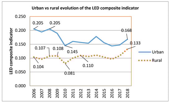
Figure 2.
Urban vs. rural evolution of composite indicator.
A deeper look into the data (see Table 7) shows that apart from two cases, all urban communities (99% of urban population) were affected by the crisis, the values during the crisis being lower than the pre-crisis values. Only 12 urban communities (towns–small urban communities—28.25% of the total urban population) registered positive values in the most recent period (recovery), compared with the crisis period. Compared with pre-crisis level, only four urban areas registered higher values in the most recent period (medium-run performers), all of them belonging to the smallest urban communities in the region.
Table 7.
Impact, recovery, and medium-run performance: a general view.
Rural communities were less affected by the crisis compared with urban ones—92 rural communities (18.66% of the total rural population of the region) had positive values during the crisis period compared with the pre-crisis period. Additionally, 327 rural communities (81.6% of the total rural population) recovered—in the most recent period, they had positive values compared with the crisis period. In total, 257 rural communities (58.3% of the total rural population) were medium-run performers; in the most recent period, they registered higher values compared with the pre-crisis level.
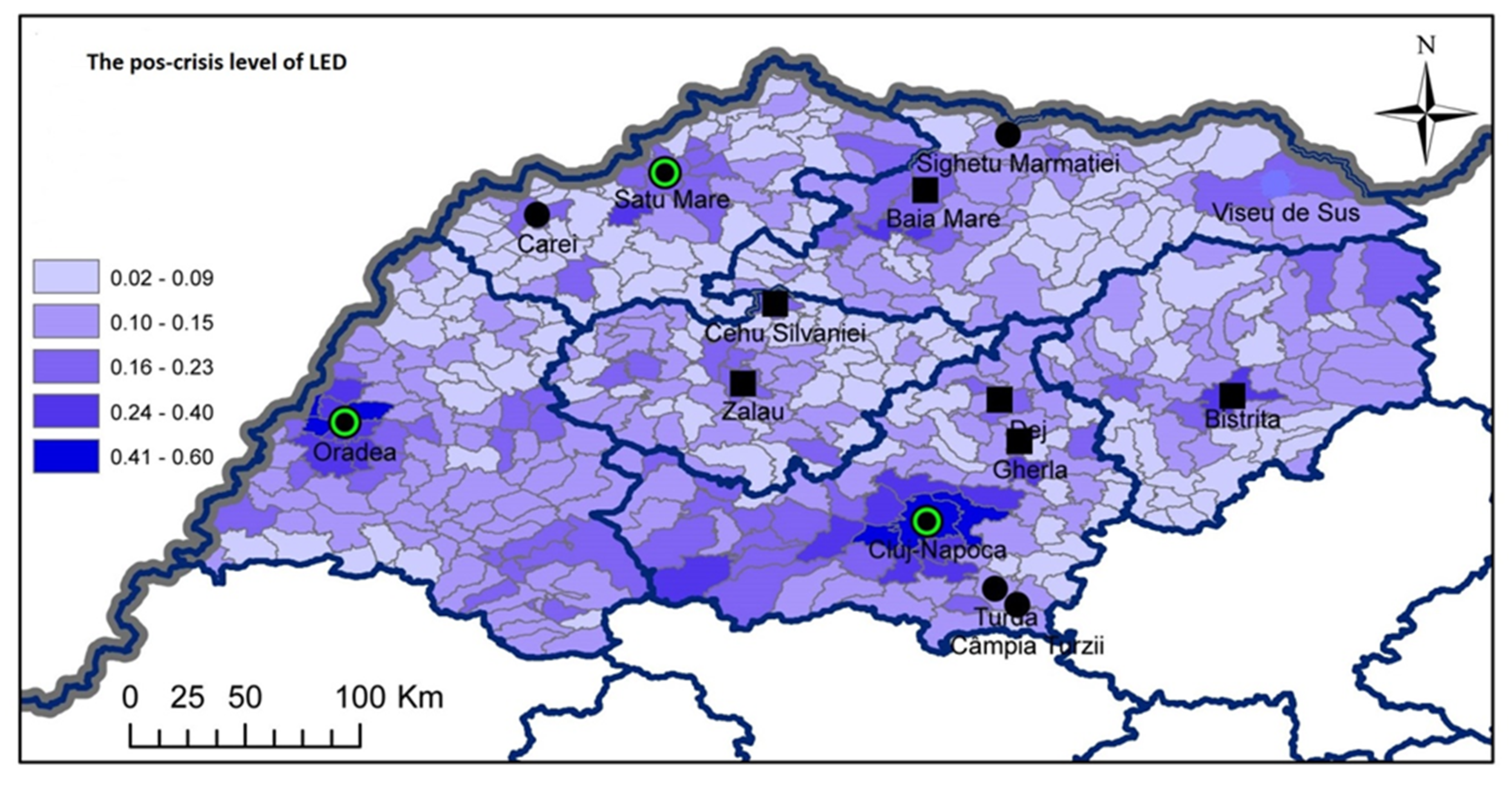
A clearer image regarding the pre-crisis and post-crisis levels of local economic development, but also regarding the impact of the crisis, the recovery, and medium-run performance (compared with the pre-crisis level) of the urban and rural communities in the region is offered in Appendix A.
3.2. Resilience Drivers for Urban and for Rural Communities (2006–2018 Period)
One of our research aims was to identify and compare the economic resilience drivers for local urban and rural communities from the North-West region of Romania. For a solid statistical–econometric analysis, we used linear regression models (cross-sectional) separately for urban and for rural communities. For urban communities (Table 8), we included in the model seven possible explanatory variables or resilience drivers. Even though the number of urban communities was low (43), all models appeared to be statistically significant (Sig. value/p-value < 0.05) and efficient (F-ratio or F), being greater than 1 for all of them. Regression models for urban communities had a weak-to-medium strength (R Square was higher than 0.03, but lower than 0.7), while for rural communities (general—all 403 communities, and Rank 1—209 communities) they were weak (R Square < 0.3). The low values of R Square registered were explained by a low variance of the independent variables having high explanatory power, as, for example, the share (very small) of university graduates, Protestants, and atheists in rural communities.
Table 8.
Summary of the regression models and economic resilience drivers for urban communities.
In order to compare the goodness-of-fit of this set of distinct but rather similar linear regression models, we used the R Square as a useful test statistic, which is often used in this context. This was certainly justified, as our regression models had a similar specification and used similar databases, the only difference being the type of communities (urban or rural, Rank 1 or Rank 6).
In the case of urban communities, when observing the impact of the crisis—the dependent variable being the difference between the worst level (2009–2011 average) and the pre-crisis level (2006–2008 average) of the LED composite indicator—communities with high shares of university graduates were the most affected by the crisis (Sig. < 0.05/Standardized Beta Coefficient, Beta being the strength of the effect of each individual independent variable to the dependent variable). These urban communities absorbed most of the economic shock. Meanwhile, urban communities with the highest share of Protestants (the only independent variable, with Sig. < 0.05) recovered less after the shock (recovery—the difference between the most recent values (2016–2018 average) and the worst level (2009–2011 average) of the LED composite indicator).
Perhaps the most surprising finding was the low recovery rate (medium-run performance) of the urban communities’ medium-term performance, the difference between the most recent level (2016–2018 average) and pre-crisis level (2006–2008 average) of the LED composite indicator. On the basis of these results, we were not able to identify significant resilience drivers for the urban communities’ resilience. None of the independent variables/predictors appeared to have stimulated the economic recovery or to have bounced forward the economy of the urban communities. Moreover, it seemed that the share of Protestants was a negative predictor for economic recovery, while the share of university graduates was a negative predictor for the medium-run performance of the local economy of these urban communities.
The collinearity diagnostic revealed that there was no collinearity between independent variables: the tolerance collinearity was higher than 0.1 (the lowest value was 0.329) and the variance inflation factor (VIF) was no greater than 10 (the max value was 3.04). Meanwhile, if we eliminated from the models the independent variables having Sig. value/p-value > 0.05, the strength of the models decreased (R Square = 0.306—Impact regression model, R Square = 0.268—Recovery regression model, R Square = 0.250—Medium-run performance regression model), but it remained statistically significant (Sig. < 0.05). It meant that the model was a satisfactory predictor of the outcome (based on an ANOVA test). At the same time, the strength of the effect of the significant predictors decreased as well (Standardized Beta Coefficient—Beta), but still remained significant (Sig. < 0.05).
In the case of rural communities (Table 9), those communities with the highest share of university graduates, those directly connected to the E-Road Network, and the biggest communities were the ones most affected by the shock—impact being the difference between the worst level (2010–2011 average) and the pre-crisis level (2007–2009 average) of the rural LED index.
Table 9.
Summary of the regression models and the drivers of economic resilience for rural communities—general level.
Meanwhile, ethnicity and religion (the share of atheists, the share of Hungarian ethnics in the population), and population size seemed to be negative predictors for economic recovery (Recovery—the dependent variable being the difference between the most recent value (2016–2018 average) and the worst level (2010–2011 average) of the LED composite indicator), while rank, the share of university graduates, and direct connection to the E-Road Network were predictors of economic recovery or resilience drivers for rural communities.
Compared with the pre-crisis level, the share of atheists, the share of Hungarian ethnics, and the population size appeared to be all negative predictors for the economic growth of rural communities, while the rank (location near a big city) was a resilience driver, predicting the medium-run performance/bounce forward of rural communities (Medium-run performance—the difference between the most recent value (2016–2018 average) and pre-crisis value (2007–2009 average) of the LED composite indicator).
None of the regression models registered collinearity between independent variables; if we eliminated independent variables having Sig. value (2-tailed)/p-value > 0.05, the models remained statistically significant (Sig. < 0.05). The strength of the effect of the significant predictors decreased too, but still remained significant.
We used the same linear regression models for Rank 1 and Rank 6 rural communities (communes) from the region (see Appendix B). We chose these communes because only their numbers were statistically large enough for linear regression: 297 Rank 1 communes and 51 Rank 6 communes.
In the case of Rank 1 communes, the communes with the highest share of atheists, the highest share of university graduates, and those directly connected to the E-Road Network were the most affected by the crisis (impact/absorption). When discussing recovery and medium-run performance, the share of Hungarian ethnics and population size were negative predictors, with no other resilience driver being identified in this case. There was no collinearity between independent variables and, if we eliminated the independent variable, the models were still significant and the predictors’ effects were significant as well.
In the case of Rank 6 communes, those with the highest share of atheists and those with the largest population size were the ones most affected by the crisis, while the Rank 6 communes directly connected to the E-Road Network were the least affected. As in the case of Rank 1 communes, in Rank 6 communes, the highest share of Hungarian ethnics and the largest population were negative predictors for economic recovery. Considering the pre-crisis level, the share of atheists, the share of Hungarian ethnics, and the largest population were negative predictors for the medium-run performance of Rank 6 communes, while university graduates and direct connection to the National Roads Network were predictors or resilience drivers. There was no collinearity between independent variables and, if we eliminated the independent variable, the models were still significant; so the predictors’ effects were significant (excepting one independent variable—Direct connection to the National Roads Network).
We also analysed the correlation between population size (pre-crisis and post-crisis levels), population change, impact, recovery, and medium-run performance values of the LED composite indicator. Population change was calculated as the difference between post-crisis population size (2016–2018 average population size) and the pre-crisis population size (2006–2009 average population size). While in the case of urban communities, there were no relevant findings, in the case of rural communities (communes of all ranks), the population change was negatively correlated with the impact of the crisis, the high values of the population change being correlated with negative values of the impact. This means that population decreased more in the most (negatively) impacted communes. It is interesting that high values of the population change were correlated with high values of recovery, meaning that the population decreased more in the communes that recovered the most after the crisis. The analysis revealed also that high values of pre-crisis population were positively correlated with the high values of the population change, meaning that the largest communes’ populations decreased the most. At the same time, the high values of the pre-crisis population size were negatively correlated with the impact, meaning that the largest communes in the region were the most affected by the crisis. Moreover, the high values of the pre-crisis population size were negatively correlated with medium-run recovery, meaning that the largest communes did not succeed in bouncing back (economically) after the economic shock.
The next step in our study analysed the evolution of the composite indicator by considering the rank of the communities. Figure 3 and Figure 4 show the evolution for both urban and rural communities.
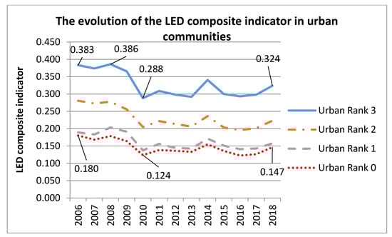
Figure 3.
The evolution of the composite indicator in urban communities (considering the rank). Source: Authors.
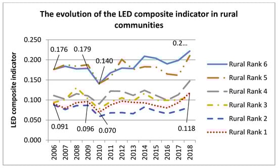
Figure 4.
The evolution of the composite indicator in rural communities (considering the rank). Source: Authors.
It was observed that, no matter the rank, all urban communities were affected by the crisis starting in 2009, and that they had not yet reached their pre-crisis level. Meanwhile, looking at the rural communities and considering their rank (we excluded the Ranks 5, 3, and 2 due to their low number and because statistically they were not representative), there was a big difference between communes situated near the largest city in the region (Rank 6) and communes situated outside the area of influence of any city (Rank 1).
The economic crisis struck all the communes (no matter their rank), starting in 2010, but Rank 6 communes (the most developed) were the most affected, the level of impact being comparable with Rank 3 urban communities, the cities in whose influencing area these communes were located.
Compared with urban communities, in the case of rural communities, no matter the rank, the decreasing trend changed suddenly (in 2011) and the growth trend continued, with some small fluctuations. But maybe the most relevant fact was that the existing difference in 2006 between Rank 6 and Rank 1 communes increased until 2018, even if the impact of the economic crisis was higher in Rank 6. From this perspective, the economic shock seemed to act as a trigger of economic development for the communes located in the influencing area of the biggest cities in the region.
3.3. Structural Shifts
Looking at medium-run regional performance, based on the absolute values of each of the indicators, we evaluated the pre-crisis structure of the regional economy (outcomes of local economy). We used in this analysis absolute values for the following indicators: turnover, employees, number of active business, number of newly created enterprises, and number of dwellings completed during the year concerned. Considering the rank of the communities, we computed the share of each indicator in the total economy for the pre-crisis period (average level for 2006–2008) and for the most recent data (average level for 2016–2018 period). In the last step, we aggregated the shares of all five indicators into a composite indicator of their shares (equal weights). The results are revealed in Table 10.
Table 10.
Pre-crisis and post-crisis shares of economic activity outcomes in the region.
Table 10 shows that, at the level of entire region, the share of the urban economy in the total economy decreased from 76% to 70% (compared with the pre-crisis), while the share of the rural economy increased from 24% to 30%. Rank 3 urban communities (the three biggest cities in the region) and the communes located in their areas of influence (Rank 6) were those whose post-crisis economic share in the total regional economy was higher than it was before the crisis. Moreover, the post-crisis share of Rank 6 communes was almost double than before the crisis, equaling the Rank 2 cities’ share in the regional economy. The indicators whose share increased the most in Rank 6 communes were the dwellings completed during the year (from 17% to 34%), active business (from 5% to 10%), and newly created enterprises (from 7% to 12%). In the case of Rank 3 cities, the indicators whose share in the total regional economy increased were dwellings completed during the year (from 28% to 43%) and number of employees (from 43% to 46%), while the share of turnover, the active business, and newly created enterprises clearly decreased. These structural shifts were more obvious if we looked at the changes (%) in the (absolute) values of the indicators (see Appendix C). The values were obtained by dividing the values of the crisis period to the pre-crisis period (impact), the values of the most recent period to the crisis period (recovery), and the values of the most recent period to the pre-crisis period (medium-run performance).
3.4. Resilience and Economic Diversity in Urban and Rank 6 Rural Communities
Using the values of the composite indicator, we evaluated the impact, recovery, and medium-run performance for the urban communities and Rank 6 rural communities (51 communes located in the influencing areas of the three biggest cities in the region), taking into account the level of economic diversity.
Based on the impact result, we constructed the ranking (classification) of the urban communities, and of the Rank 6 communes (see Appendix D). In the case of urban communities, with some exceptions, the largest cities of the regions, Rank 3 and 2 cities (those with the highest level of economic diversity in 2008), were the ones most affected by the economic crisis. The least diversified, inherently small-sized, and least-developed urban communities were less affected. At the same time, a change in the economic structure seemed to have occurred after the crisis. The share of services in the total economy increased in the most affected urban communities, while the share of industries apparently decreased. The situation was the opposite in the less affected urban communities after the crisis.
Looking at the recovery of the urban communities, except for an outlier (the largest and most developed city in the region), the highest recovery was registered in the less impacted urban communities. At the same time, the largest and most developed urban communities in the region (Rank 3 and 2) seemed to have recovered the least after the crisis.
Looking at the economic diversity, no trend or structural path was identified in urban communities. Compared with the pre-crisis level (medium-run performance), the situation was the same as in the case of recovery. The only significant observation concerned the change in the structure of the local economy in the case of all three Rank 3 cities (the biggest cities in the region), where the share of services in the local economy was (the most recent years) higher compared with the pre-crisis level.
In the case of Rank 6 communes, with some exceptions, the communes with the highest level of economic diversity (computed using the Hachman Index) in 2008 were the ones most affected by the crisis. In terms of diversification of economic structure, no relevant changes occurred in the analysis period, the communes with the highest economic diversity being the same ones at the beginning as well as in 2017. In terms of structural shifts, an increase in the share of services sectors (+9.17% from 2008 to 2017), agriculture (+2.1%) and industry (+1.7%) occurred, at the expense of construction and trade sectors.
Rank 6 communes with the highest bounce-back values were the ones with the highest level of diversification recorded in 2008. Meanwhile, the highest recovery was registered in the communes with the highest increase in services sector share. This was valid and more accentuated in the case of medium-run performers—those communes were the ones with the highest growth of the share of the services sector.
The changes and shifts produced in the structure of the economy of the urban communities and of the most developed rural communities (Rank 6 communes—those located nearest the largest cities in the region) were more obvious if we looked at the absolute values of the employees in the last year before the crisis (2008) and the most recent year (2018). Table 11 reveals better these changes:
Table 11.
Changes in economic structure in 2008–2018: Number of employees in urban communities and Rank 6 communes.
In the case of urban communities, all the sectors except the services sector registered in 2018 a lower number of employees than in 2008. Meanwhile, in the communes located near the largest and most developed cities in the region, the number of employees increased significantly in industry (+64.00%) and services (+89.63%) sectors.
4. Discussion
In light of the findings above, the engines for economic recovery in the region seem to be the communes located near the largest cities. These communes bounced forward, changing their local economic structure by increasing the shares of services, industry, and agriculture sectors. Meanwhile, the largest cities in the region changed their economic structure, as well, the services sector becoming the most important sector in the local economy. Thus, the largest cities became service centres (financial and economic, education, health, research, culture and recreation, etc.) or creative industry centres of the region. Hence, the communes located in their vicinity became virtual spread areas for the expansion of the economic activity of urban/metropolitan areas to be ‘economically contaminated’, becoming preferred destination locations for industries and service activities.
From a policy perspective, the findings of the study can be used as a base for future regional development plans, national sectoral development policy, sustainable urban mobility, transport infrastructure policy (highways and railways for connectivity), education policy, rural development policy, etc. Clearly, the spatial context/pattern of interactions in the case of production, distribution, or consumption systems matters, as well as the importance of the management, planning, and forecasting of spatial development [68].
At the local level, our findings may be relevant for the decision-making process, considering the structural changes of the local economies of the biggest cities and the communes in their vicinity. In the light of the last economic crisis, it seems likely that the biggest cities and the communes around them might be vulnerable to the next crisis, but also that they have the potential to recover the most and to bounce their economy forward by adapting to the global trend and new challenges, changing the structure of their local economies, and using the opportunities created by global changes more efficiently.
5. Conclusions
The aim of this study was to assess the differences in the economic resilience of rural and urban communities from the North-West region of Romania and to identify the drivers of economic resilience for these communities. Using a composite indicator that aggregates proxies (mainly outcomes) for different components of the local economic development, namely, the strength of economic activity, the level of productivity, the intensity of economic activity, entrepreneurial initiatives, and real estate market and attractiveness, we addressed the following questions: How much has the financial and economic crisis affected local communities? How well have communities recovered from the crisis? What is the current situation in the communities compared with the pre-crisis one?
Our study both confirms and rejects—fully or partially—various assumptions. The first assumption is fully confirmed: the economic crisis hit urban communities earlier than the rural communities. While the rural communities were less and later affected, they started to recover earlier and more than urban communities, the difference between urban and rural gradually narrowing after the crisis. But a supplementary explanation is necessary here. A deeper analysis into rural communities reveals that not all rural communities were affected in an equal manner by the economic shock. Thus, rural communities located nearest the biggest cities in the region (Rank 6 communes), were strongly affected by the economic crisis, while the most isolated rural communities (Rank 1 communes) were the least affected.
The second assumption is entirely rejected, as rural communities appear to be more resilient than urban ones, but there are some important exceptions. Not all rural communities have the same level of resilience. Rural communities located in the influencing area/vicinity of the biggest cities in the region were affected the most by the crisis, but, at the same time, they grew the most when compared with their crisis and pre-crisis levels, being the high performers of the period. At the same time, the isolated rural communities (less developed, small and medium-size, beyond any city’s influence area) were the least affected by the crisis, but their growth rate was the lowest. An explanation could be the pre-existent level of economic development (predominantly agrarian and mainly autarchic/self-sufficient) and a low level of interconnectedness with the global economy.
The third assumption is fully confirmed in the case of rural communities and partially confirmed in the case of urban communities. Moreover, their rank is a resilience driver for rural communities: those located in the influencing area/vicinity of the biggest cities in the region grew the most compared with their crisis and pre-crisis levels, being the high performers of the period. The economies of these communes bounced apparently forward.
Regarding the fourth hypothesis, there are some relevant findings and conclusions to be mentioned: whether or not urban or rural communities with the highest share of university graduates were significantly affected by the economic crisis.
In the case of urban communities, the share of Protestants seemed to be a negative predictor for the recovery after the crisis, while the share of university graduates seemed to be a negative predictor for the economic growth compared with the pre-crisis level.
Rural communities with the highest share of university graduates, those connected to the E-Road Network, and those with the largest population were the most significantly affected by the crisis.
In the case of the rural communities, the share of Protestants, the share of atheists, the size of the population, and the share of university graduates were negative predictors, for both the crisis level (recovery) and the pre-crisis level (medium-run performance), while the rank of the communes and direct connection to the E-Road Network were predictors for growth compared with the crisis level; the direct connection to E-Road Network was a resilience driver for rural communities, which have the highest growth compared with their pre-crisis level.
Whether urban or rural, and no matter the rank of the community, the capital investment of local authorities did not succeed in mitigating the impact of the crisis, nor in stimulating recovery or medium-run performance.
Economic diversity did not appear as a resilience driver for urban communities. Moreover, it seems that the cities with diversified economies were affected the most by the crisis; in these cities the share of services in the total economy increased after the crisis, while the share of industry decreased.
In line with our findings regarding the recovery rate, [34] stress that regions that performed well before the crisis were not able to achieve a quicker recovery, while [12] observe that developed counties recover more quickly after the economic shocks, but the typology of economic recovery illustrates a variety of situations, depending on the indicator taken into consideration as a measure for resilience (GDP or employment). However, our analysis goes deeper into the administrative layering, attempting to identify resilient administrative units at the lowest level.
The results concerning the share of university graduates are not similar to other research on Romania, which reconfirmed its positive role in the economic performance of the regions [14], but at the same time they could be explained by the findings of the same study [14], which show that developed administrative units (counties in this case) were the most affected by economic crisis. In these counties, the international trade and the investment inflows dropped sharply during the crisis. Concerning diversification, the same research found that the more diversified the Romanian counties were, the better they were at coping with the economic shocks, but one of the limits of this research was the fact that the analysis was made from an aggregated regional perspective. The proxies used for the level of regional development (GDP, industrialization, and urbanization) prompted a higher vulnerability level to economic shocks for the more developed counties—supporting our findings related to the impact of the crisis inside the North-West region. Another source of differentiation between the results (less likely, though) might be the instrument used in assessing diversity (Hachman index vs. Krugman and Herfindahl). Although when choosing the variable we assumed that a high percentage of the Protestant religion population might be a descriptor for resilience, the results show that the indicator was a negative predictor for the communities’ recovery. Our results are opposite to post-Weberian findings of other research showing that Protestantism is associated with higher levels of economic development/lower unemployment rates/labor force participation [41], or identifying significant differences in economic outcomes of Romanians according to religious affiliation [42].
In the same manner, we considered that the percentage of Hungarians could be a predictor, as they are known to have a work ethic superior to other ethnic groups in the region, compounded by the fact that the majority of them are of Reformed religion (Protestants). Analysing the situation from both perspectives would have allowed us to better understand the situation, as long as the large majority of Hungarian ethnics are of Reformed (Protestant) religion. This would have helped us to control for inconsistent results, if one of the variables turned out to be a resilience driver (e.g., Hungarian ethnics’ share of the population).
One explanation for the results could be the population breakdown of the Protestant religion, with Pentecostals representing the second largest part, after the Reformed. As Foszto and Kiss [69] noticed, based on an analysis of statistical data, the Pentecostal population is concentrated in the North-West region, especially in the border counties, with an overrepresentation of rural population (60%) and of Roma ethnics, suggesting that disadvantaged population classes are unevenly distributed compared to the other ones. Those two categories are associated with higher levels of poverty.
One of the most important findings of the study is related to the shift in terms of the economic structure. The crisis triggered a structural change in the economy of the region, whereby part of the activity was relocated from the urban to the rural areas (especially those located in the vicinity of large cities). However, there is no proof that this was a response to a shock or just the natural evolution of the metropolitan areas (in this context the role of the metropolitan areas is more important than ever). From a resilience perspective, this could be similar to Martin’s adaptive resilience—‘the ability of a system to implement reorganization of the system’s structure, so as to minimize the extent of the disturbance affecting the system, or to take advantage of the shock to achieve renewal of the system’ [9].
It may finally be noted that public organisations (including communes and regions) are expected to perform at high levels while constantly improving and adapting to the changing dynamics of the socioeconomic environment [68,70], including addressing and mitigating shocks. In light of our findings we may argue that strategic planning is an essential tool in developing the capacities of communities to respond to external factors [71]. Strategic approaches should be concentrated on specific areas, like entrepreneurship and support for SMEs (see [72]).
As communities with a stronger bonding capital may be able to overcome periods of distress more easily [73], a lesson for local authorities may be to strengthen the ties and tolerance among the residents in order to increase their resilience level. This is a valid approach, especially in the North-West region, which has a high level of ethnic and religious diversity.
Clearly, there are also some main limitations in our research. The first concerns the metrics used for measuring the resilience. As we mentioned, one of the most important issues in the field is whether to use a single proxy or a composite indicator to measure resilience. Another limitation may be the use of the indicator ‘Number of dwellings completed during the year (per 1000 inhabitants)’. This is a lagging indicator due to the necessary time of completion, and therefore the impact of the crisis in this case may not be immediately visible. This limitation is mitigated by the fact that after a period of continuing growth (2006–2008), in 2009, compared with 2008, this indicator registered a significantly lower value, whether for urban (−11.08%) or rural (−18.42%) communities. The adapted JRC approach for measuring resilience based only on outcomes could be another limitation of our research. Using different variables for rural and for urban communities might be another limitation of the study, as well as the absence of a spatial model for a more appropriate analysis of the economic resilience of local communities, considering the location factor. Moreover, a pooled estimation model with panel data would get more accuracy in our research results. But these will be the new endeavours and opportunities for future research in the field.
Most of the results of our study may be extrapolated to other local communities from Romania. There are some explanatory variables that could or should be replaced with others, for example, the share of Hungarian ethnics or the share of Protestants, because Hungarians represent a strong ethnic group in three out of all eight development regions of Romania.
Future research is necessary to examine whether the bounce-forward phenomenon of the communes located in the influencing areas of the largest cities is caused by resilience, or whether native ‘prosilience’ represents a general trend for southeastern European/ex-communist countries, whose urbanisation process was begun during the communist period. Moreover, when analysing the evolution of the economic structure of the communes positioned in the immediate vicinity of large cities, it is necessary to provide a more comprehensive and significant explanation for the changes that occurred in their economic path. The big cities and the communes around them were not naturally (from an economic and urbanistic point of view) interconnected and integrated as a functional metropolitan area. They were artificially separated by the urban communities nearby, which, in the context of free market and globalisation, is generally not efficient. It is clear that the study on resilience of urban–rural systems needs insights from various branches of geography: social, urban, rural, economic, and cultural.
Author Contributions
Conceptualization, A.P. and B.A.M.; methodology, A.P.; software, SPSS 20, Microsoft Excel, GIS, A.P. and B.A.M.; validation, A.P., B.A.M., P.N. and K.K.; formal analysis, A.P.; investigation, A.P.; resources, A.P. and B.A.M.; data curation, A.P. and B.A.M.; writing—original draft preparation, A.P. and B.A.M.; writing—review and editing, P.N. and K.K.; visualization, K.K.; supervision, P.N. and K.K. All authors have read and agreed to the published version of the manuscript.
Funding
This study was funded by the Romanian Executive Unit for Financing Higher Education, Research, Development and Innovation (UEFISCDI) through the project Dezvoltarea cercetării de frontieră în teoriile creșterii și dezvoltării regionale prin prisma rezilienței: către o Uniune Europeană convergentă, echilibrată și sustenabilă (project code: PN-III-P4-ID-PCCF-2016-0166) implemented by Alexandru Ioan-Cuza University of Iași, regroweu@uaic.ro.
Conflicts of Interest
The authors declare no conflict of interest.
Appendix A. GIS Presentation of the Evolution of the North-West Region
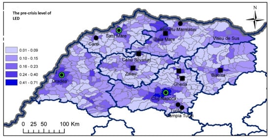
Figure A1.
Pre-crisis LED level; source: Authors.
Figure A1.
Pre-crisis LED level; source: Authors.
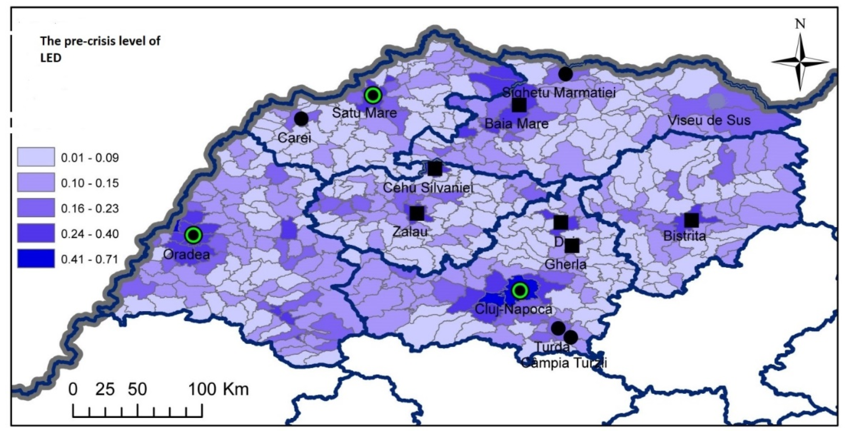
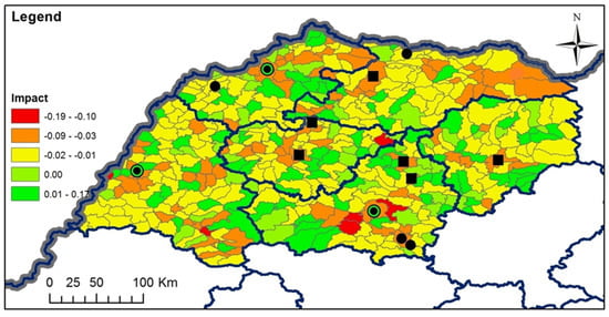
Figure A2.
Impact of the crisis; source: Authors.
Figure A2.
Impact of the crisis; source: Authors.

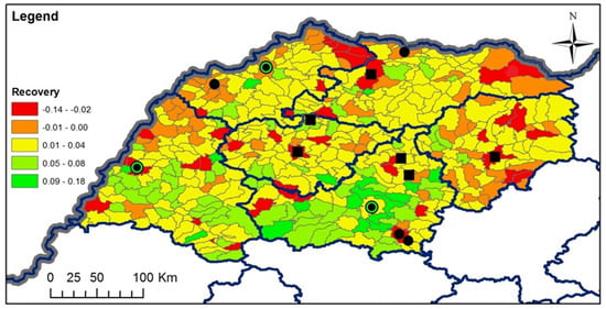
Figure A3.
Recovery from crisis; source: Authors.
Figure A3.
Recovery from crisis; source: Authors.
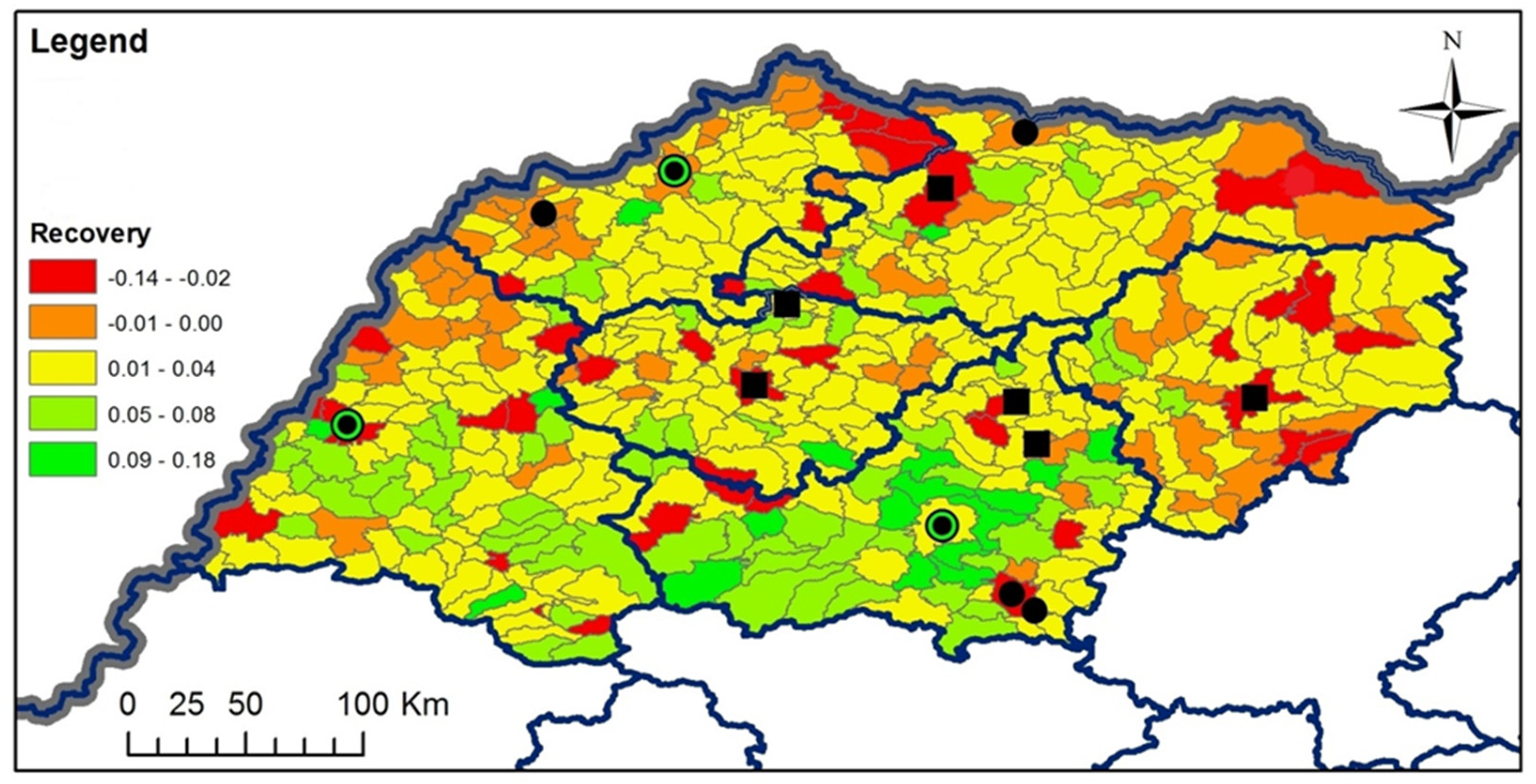
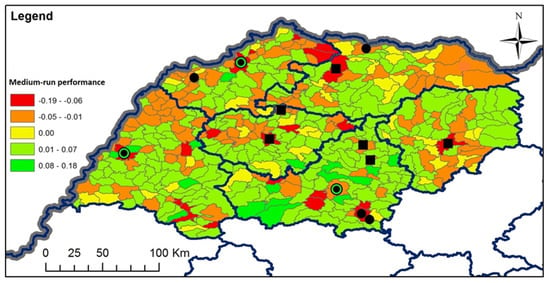
Figure A4.
Medium-run performance; source: Authors.
Figure A4.
Medium-run performance; source: Authors.
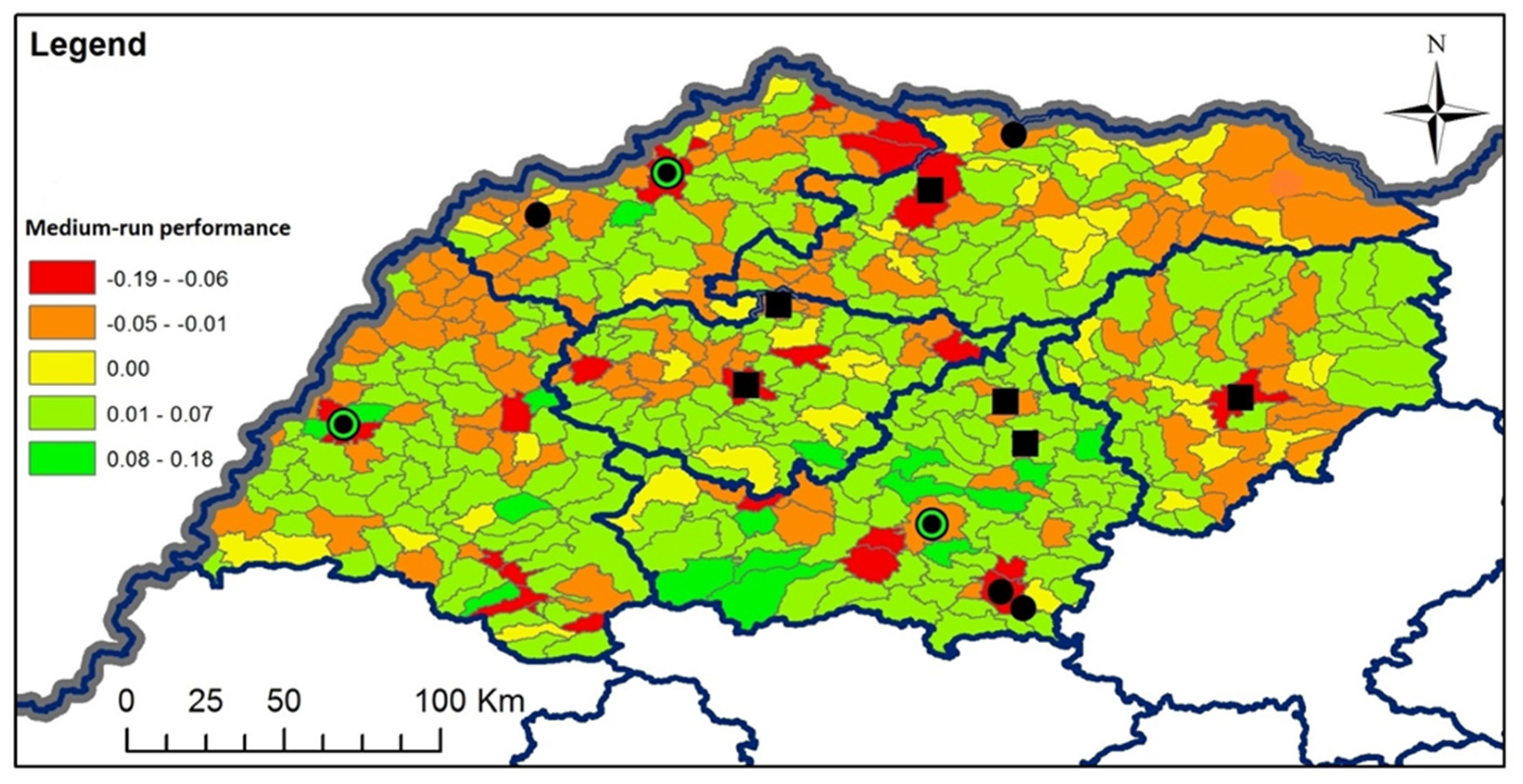
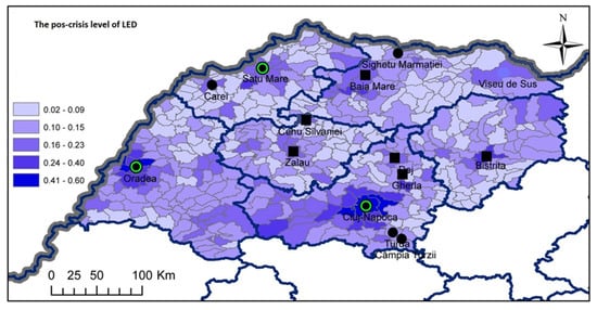
Figure A5.
Post-crisis LED level; source: Authors.
Figure A5.
Post-crisis LED level; source: Authors.
.
Appendix B. Summary Statistics
Table A1.
Summary of regression models and drivers of economic resilience for rural communities—Rank 1 communities.
Table A1.
Summary of regression models and drivers of economic resilience for rural communities—Rank 1 communities.
| Indicator | Dependent Variable | Independent Variables | B | Std. Error | Beta | t | Sig. | R Square | R | F | Sig. |
|---|---|---|---|---|---|---|---|---|---|---|---|
| LED composite indicator | Impact | Share of Protestants | −0.041 | 0.033 | −0.074 | −1.241 | 0.216 | 0.099 | 0.314 | 3.496 | 0.000 |
| Share of atheists | −19.672 | 9.276 | −0.121 | −2.121 | 0.035 | ||||||
| Share of Hungarian ethnics | −0.001 | 0.006 | −0.009 | −0.144 | 0.885 | ||||||
| Share of university graduates | −0.222 | 0.090 | −0.147 | −2.456 | 0.015 | ||||||
| Share of capital investment 2006–2008 | −0.001 | 0.014 | −0.006 | −0.100 | 0.921 | ||||||
| Share of capital investment 2009–2011 | −0.012 | 0.013 | −0.060 | −0.954 | 0.341 | ||||||
| Direct connection to the E-Road Network | −0.008 | 0.004 | −0.131 | −2.194 | 0.029 | ||||||
| Direct connection to the National Roads Network | 0.000 | 0.004 | 0.002 | 0.028 | 0.977 | ||||||
| Population size (pre-crisis) | 0.000 | 0.000 | −0.066 | −1.084 | 0.279 | ||||||
| Recovery | Share of Protestants | 0.014 | 0.038 | 0.022 | 0.368 | 0.713 | 0.094 | 0.307 | 3.325 | 0.001 | |
| Share of atheists | 5.156 | 10.648 | 0.028 | 0.484 | 0.629 | ||||||
| Share of Hungarian ethnics | −0.027 | 0.007 | −0.220 | −3.634 | 0.000 | ||||||
| Share of university graduates | 0.140 | 0.104 | 0.082 | 1.357 | 0.176 | ||||||
| Share of capital investment 2006–2008 | −0.005 | 0.016 | −0.022 | −0.343 | 0.732 | ||||||
| Share of capital investment 2009–2011 | 0.012 | 0.015 | 0.052 | 0.816 | 0.415 | ||||||
| Direct connection to the E-Road Network | 0.008 | 0.004 | 0.115 | 1.935 | 0.054 | ||||||
| Direct connection to the National Roads Network | 0.001 | 0.004 | 0.010 | 0.175 | 0.861 | ||||||
| Population size (pre-crisis) | 0.000 | 0.000 | −0.182 | −2.978 | 0.003 | ||||||
| Medium-run performance | Share of Protestants | −0.027 | 0.042 | −0.038 | −0.638 | 0.524 | 0.110 | 0.332 | 3.941 | 0.000 | |
| Share of atheists | −14.518 | 11.786 | −0.070 | −1.232 | 0.219 | ||||||
| Share of Hungarian ethnics | −0.028 | 0.008 | −0.203 | −3.387 | 0.001 | ||||||
| Share of university graduates | −0.083 | 0.115 | −0.043 | −0.725 | 0.469 | ||||||
| Share of capital investment 2006–2008 | −0.007 | 0.018 | −0.026 | −0.397 | 0.692 | ||||||
| Share of capital investment 2009–2011 | 0 | 0.016 | 0.000 | −0.004 | 0.997 | ||||||
| Direct connection to the E-Road Network | 0.000 | 0.005 | 0.003 | 0.046 | 0.963 | ||||||
| Direct connection to the National Roads Network | 0.001 | 0.005 | 0.010 | 0.169 | 0.866 | ||||||
| Population size (pre-crisis) | 0.000 | 0.000 | −0.215 | −3.548 | 0.000 |
Source: Authors.
Table A2.
Summary of regression models and drivers of economic resilience for rural communities—Rank 6 communities.
Table A2.
Summary of regression models and drivers of economic resilience for rural communities—Rank 6 communities.
| Indicator | Dependent Variable | Independent Variables | B | Std. Error | Beta | t | Sig. | R Square | R | F | Sig. |
|---|---|---|---|---|---|---|---|---|---|---|---|
| LED composite indicator | Impact | Share of Protestants | −0.024 | 0.074 | −0.041 | −0.326 | 0.746 | 0.373 | 0.610 | 2.705 | 0.014 |
| Share of atheists | −33.500 | 13.806 | −0.490 | −2.427 | 0.020 | ||||||
| Share of Hungarian ethnics | −0.008 | 0.022 | −0.048 | −0.363 | 0.719 | ||||||
| Share of university graduates | 0.303 | 0.158 | 0.424 | 1.918 | 0.062 | ||||||
| Share of capital investment 2006–2008 | 0.012 | 0.063 | 0.027 | 0.191 | 0.849 | ||||||
| Share of capital investment 2009–2011 | −0.116 | 0.060 | −0.301 | −1.941 | 0.059 | ||||||
| Direct connection to the E-Road Network | −0.019 | 0.012 | −0.222 | −1.594 | 0.119 | ||||||
| Direct connection to the National Roads Network | 0.036 | 0.017 | 0.301 | 2.091 | 0.043 | ||||||
| Population size (pre-crisis) | 0.000 | 0.000 | −0.340 | −2.028 | 0.049 | ||||||
| Recovery | Share of Protestants | −0.088 | 0.077 | −0.145 | −1.153 | 0.255 | 0.382 | 0.618 | 2.813 | 0.011 | |
| Share of atheists | −23.930 | 14.235 | −0.337 | −1.681 | 0.100 | ||||||
| Share of Hungarian ethnics | −0.077 | 0.023 | −0.447 | −3.405 | 0.001 | ||||||
| Share of university graduates | 0.299 | 0.163 | 0.403 | 1.837 | 0.073 | ||||||
| Share of capital investment 2006–2008 | 0.023 | 0.065 | 0.048 | 0.348 | 0.730 | ||||||
| Share of capital investment 2009–2011 | 0.071 | 0.062 | 0.176 | 1.146 | 0.258 | ||||||
| Direct connection to the E-Road Network | 0.008 | 0.012 | 0.091 | 0.658 | 0.514 | ||||||
| Direct connection to the National Roads Network | 0.037 | 0.018 | 0.298 | 2.083 | 0.044 | ||||||
| Population size (pre-crisis) | 0.000 | 0.000 | −0.160 | −0.963 | 0.341 | ||||||
| Medium-run performance | Share of Protestants | −0.113 | 0.103 | −0.135 | −1.089 | 0.283 | 0.395 | 0.628 | 2.971 | 0.008 | |
| Share of atheists | −57.561 | 19.211 | −0.594 | −2.996 | 0.005 | ||||||
| Share of Hungarian ethnics | −0.085 | 0.030 | −0.362 | −2.792 | 0.008 | ||||||
| Share of university graduates | 0.603 | 0.220 | 0.596 | 2.744 | 0.009 | ||||||
| Share of capital investment 2006–2008 | 0.035 | 0.088 | 0.055 | 0.396 | 0.694 | ||||||
| Share of capital investment 2009–2011 | −0.045 | 0.083 | −0.082 | −0.537 | 0.594 | ||||||
| Direct connection to the E-Road Network | −0.011 | 0.017 | −0.090 | −0.660 | 0.513 | ||||||
| Direct connection to the National Roads Network | 0.073 | 0.024 | 0.430 | 3.040 | 0.004 | ||||||
| Population size (pre-crisis) | 0.000 | 0.000 | −0.359 | −2.181 | 0.035 |
Source: Authors.
Appendix C. Changes in Absolute Values of the Individual Indicators Used for Measuring Local Economy
| % Change in Turnover (Real Values) | |||
| Impact | Recovery | Medium-run Performance | |
| Total | 103.57% | 126.38% | 130.90% |
| Urban | 100.81% | 119.17% | 120.14% |
| Rural | 112.36% | 172.52% | 193.84% |
| Urban Rank 0 | 99.56% | 126.22% | 125.67% |
| Urban Rank 1 | 99.67% | 119.30% | 118.90% |
| Urban Rank 2 | 85.17% | 133.63% | 113.82% |
| Urban Rank 3 | 106.75% | 113.97% | 121.67% |
| Rural Rank 1 | 110.90% | 162.81% | 180.55% |
| Rural Rank 2 | 107.71% | 202.31% | 217.91% |
| Rural Rank 3 | 103.75% | 235.99% | 244.84% |
| Rural Rank 4 | 90.28% | 173.13% | 156.30% |
| Rural Rank 5 | 92.62% | 112.48% | 104.17% |
| Rural Rank 6 | 118.66% | 182.11% | 216.09% |
| % Change in Employees (Absolute Values) | |||
| Impact | Recovery | Medium-run Performance | |
| Total | 93.83% | 115.10% | 107.99% |
| Urban | 92.45% | 113.47% | 104.91% |
| Rural | 101.39% | 121.92% | 123.62% |
| Urban Rank 0 | 88.33% | 106.06% | 93.68% |
| Urban Rank 1 | 87.65% | 86.24% | 75.59% |
| Urban Rank 2 | 89.02% | 110.69% | 98.54% |
| Urban Rank 3 | 96.10% | 120.53% | 115.83% |
| Rural Rank 1 | 95.95% | 116.31% | 111.60% |
| Rural Rank 2 | 96.84% | 119.89% | 116.10% |
| Rural Rank 3 | 110.74% | 120.69% | 133.65% |
| Rural Rank 4 | 103.14% | 123.58% | 127.47% |
| Rural Rank 5 | 108.15% | 139.49% | 150.86% |
| Rural Rank 6 | 114.37% | 132.49% | 151.54% |
| % Change in Number of Active Enterprises (Absolute Values) | |||
| Impact | Recovery | Medium-run Performance | |
| Total | 102.08% | 116.80% | 119.23% |
| Urban | 100.23% | 107.71% | 107.96% |
| Rural | 106.56% | 157.78% | 168.12% |
| Urban Rank 0 | 98.13% | 106.57% | 104.58% |
| Urban Rank 1 | 98.39% | 102.26% | 100.61% |
| Urban Rank 2 | 98.41% | 96.82% | 95.29% |
| Urban Rank 3 | 101.64% | 113.01% | 114.86% |
| Rural Rank 1 | 104.10% | 137.91% | 143.57% |
| Rural Rank 2 | 94.40% | 128.37% | 121.18% |
| Rural Rank 3 | 109.89% | 147.90% | 162.52% |
| Rural Rank 4 | 103.40% | 149.15% | 154.22% |
| Rural Rank 5 | 105.62% | 137.91% | 145.66% |
| Rural Rank 6 | 113.37% | 202.73% | 229.83% |
| % Change in Entrepreneurial Capacity/Newly-created Enterprises (Absolute Values) | |||
| Impact | Recovery | Medium-run Performance | |
| Total | 85.09% | 104.76% | 89.14% |
| Urban | 70.18% | 103.99% | 72.97% |
| Rural | 115.68% | 114.98% | 133.01% |
| Urban Rank 0 | 75.74% | 93.72% | 70.98% |
| Urban Rank 1 | 72.29% | 88.54% | 64.00% |
| Urban Rank 2 | 75.16% | 99.73% | 74.96% |
| Urban Rank 3 | 66.50% | 111.10% | 73.89% |
| Rural Rank 1 | 125.73% | 102.28% | 128.60% |
| Rural Rank 2 | 109.78% | 79.71% | 87.50% |
| Rural Rank 3 | 87.57% | 107.35% | 94.01% |
| Rural Rank 4 | 110.03% | 114.32% | 125.78% |
| Rural Rank 5 | 108.73% | 102.75% | 111.72% |
| Rural Rank 6 | 96.73% | 160.87% | 155.61% |
| % Change in Total Number of Dwellings Completed During the Year (Absolute Values) | |||
| Impact Urban | Recovery Urban | Medium-run Performance | |
| Total | 205.35% | 108.97% | 223.78% |
| Urban | 159.55% | 137.37% | 219.17% |
| Rural | 294.16% | 78.23% | 230.12% |
| Urban Rank 0 | 153.95% | 54.67% | 84.16% |
| Urban Rank 1 | 151.43% | 62.78% | 95.06% |
| Urban Rank 2 | 159.17% | 75.24% | 119.76% |
| Urban Rank 3 | 163.36% | 211.04% | 344.76% |
| Rural Rank 1 | 150.78% | 55.91% | 84.30% |
| Rural Rank 2 | 277.83% | 21.60% | 60.00% |
| Rural Rank 3 | 99.46% | 79.78% | 79.35% |
| Rural Rank 4 | 145.45% | 59.85% | 87.04% |
| Rural Rank 5 | 131.34% | 96.49% | 126.73% |
| Rural Rank 6 | 498.36% | 87.47% | 435.92% |
Appendix D. Ranking Result
Green is for positive values (>0), red is for negative values (<0). The intensity of the shades depends by the size of the values.
Table A3.
Ranking of urban communities based on the impact of the crisis: link with economic diversity.
Table A3.
Ranking of urban communities based on the impact of the crisis: link with economic diversity.
| City/town | Urban Rank | Impact | Hachman Index 2008 | Hachman Index 2017 | Dif. Hachman 2017–2008 | Modif. Industry | Modif. Construction | Modif. Trade | Modif. Services |
|---|---|---|---|---|---|---|---|---|---|
| ORAŞ ŞTEI | 0 | −0.079 | 0.374 | 0.633 | 0.259 | −0.228 | −0.005 | 0.087 | 0.142 |
| MUNICIPIUL ZALĂU | 2 | −0.071 | 0.869 | 0.874 | 0.005 | −0.042 | −0.025 | 0.010 | 0.114 |
| MUNICIPIUL CLUJ−NAPOCA | 3 | −0.066 | 0.804 | 0.676 | −0.128 | −0.048 | −0.049 | −0.052 | 0.208 |
| ORAŞ ALEŞD | 0 | −0.063 | 0.529 | 0.687 | 0.158 | −0.153 | 0.002 | 0.036 | 0.137 |
| MUNICIPIUL ORADEA | 3 | −0.058 | 0.882 | 0.898 | 0.015 | 0.052 | −0.028 | −0.107 | 0.162 |
| MUNICIPIUL SATU MARE | 3 | −0.057 | 0.771 | 0.810 | 0.039 | 0.000 | −0.037 | 0.010 | 0.087 |
| ORAŞ SĂLIŞTEA DE SUS | 0 | −0.056 | 0.285 | 0.422 | 0.137 | −0.194 | 0.040 | 0.140 | 0.105 |
| MUNICIPIUL BISTRIŢA | 2 | −0.054 | 0.715 | 0.692 | −0.023 | 0.052 | −0.045 | −0.044 | 0.088 |
| MUNICIPIUL GHERLA | 2 | −0.053 | 0.661 | 0.624 | −0.037 | 0.124 | −0.101 | −0.041 | 0.060 |
| ORAŞ DRAGOMIREŞTI | 0 | −0.051 | 0.506 | 0.401 | −0.106 | −0.530 | 0.283 | 0.008 | 0.304 |
| MUNICIPIUL BEIUŞ | 0 | −0.050 | 0.713 | 0.783 | 0.070 | −0.134 | −0.027 | 0.080 | 0.102 |
| ORAŞ JIBOU | 0 | −0.050 | 0.654 | 0.687 | 0.033 | −0.014 | −0.023 | −0.075 | 0.184 |
| ORAŞ NEGREŞTI−OAŞ | 0 | −0.049 | 0.215 | 0.365 | 0.150 | 0.003 | −0.052 | 0.010 | 0.052 |
| MUNICIPIUL DEJ | 2 | −0.049 | 0.807 | 0.842 | 0.035 | −0.019 | −0.014 | −0.079 | 0.178 |
| ORAŞ BECLEAN | 0 | −0.047 | 0.634 | 0.781 | 0.147 | −0.228 | 0.036 | 0.067 | 0.196 |
| MUNICIPIUL TURDA | 1 | −0.046 | 0.806 | 0.781 | −0.025 | −0.023 | −0.016 | −0.053 | 0.152 |
| MUNICIPIUL MARGHITA | 0 | −0.044 | 0.573 | 0.652 | 0.080 | −0.021 | −0.025 | 0.001 | 0.104 |
| ORAŞ SEINI | 0 | −0.043 | 0.766 | 0.647 | −0.119 | −0.053 | 0.010 | 0.055 | 0.001 |
| MUNICIPIUL BAIA MARE | 2 | −0.042 | 0.800 | 0.879 | 0.079 | 0.021 | −0.050 | −0.017 | 0.094 |
| ORAŞ VAŞCĂU | 0 | −0.041 | 0.468 | 0.607 | 0.139 | −0.158 | −0.016 | 0.039 | 0.197 |
| ORAŞ NUCET | 0 | −0.037 | 0.549 | 0.083 | −0.466 | 0.166 | 0.024 | −0.276 | 0.020 |
| ORAŞ VIŞEU DE SUS | 0 | −0.035 | 0.710 | 0.717 | 0.007 | −0.027 | −0.012 | −0.040 | 0.111 |
| ORAŞ ŞIMLEU SILVANIEI | 0 | −0.035 | 0.728 | 0.778 | 0.050 | 0.012 | −0.011 | −0.079 | 0.150 |
| ORAŞ LIVADA | 0 | −0.034 | 0.602 | 0.615 | 0.013 | 0.009 | 0.027 | −0.037 | −0.028 |
| ORAŞ BORŞA | 0 | −0.033 | 0.579 | 0.593 | 0.014 | 0.011 | 0.117 | −0.095 | 0.070 |
| ORAŞ CAVNIC | 0 | −0.032 | 0.619 | 0.598 | −0.020 | −0.131 | 0.137 | 0.174 | −0.036 |
| MUNICIPIUL CÂMPIA TURZII | 1 | −0.032 | 0.631 | 0.800 | 0.168 | −0.156 | 0.021 | 0.028 | 0.119 |
| ORAŞ BAIA SPRIE | 0 | −0.031 | 0.690 | 0.712 | 0.023 | −0.040 | −0.039 | −0.039 | 0.173 |
| ORAŞ ŞOMCUTA MARE | 0 | −0.030 | 0.727 | 0.766 | 0.039 | −0.117 | −0.040 | 0.065 | 0.142 |
| MUNICIPIUL SIGHETU MARMAŢIEI | 1 | −0.030 | 0.666 | 0.654 | −0.012 | 0.051 | −0.024 | −0.021 | 0.048 |
| MUNICIPIUL SALONTA | 0 | −0.028 | 0.645 | 0.657 | 0.012 | 0.055 | −0.034 | −0.064 | 0.071 |
| ORAŞ HUEDIN | 0 | −0.025 | 0.785 | 0.728 | −0.057 | −0.094 | 0.001 | 0.025 | 0.199 |
| ORAŞ VALEA LUI MIHAI | 0 | −0.023 | 0.383 | 0.403 | 0.020 | 0.009 | −0.010 | −0.004 | 0.019 |
| ORAŞ CEHU SILVANIEI | 0 | −0.021 | 0.479 | 0.499 | 0.020 | 0.017 | −0.034 | −0.018 | 0.031 |
| ORAŞ TĂUŢII−MĂGHERĂUŞ | 0 | −0.021 | 0.646 | 0.605 | −0.042 | 0.062 | 0.002 | 0.011 | 0.068 |
| MUNICIPIUL CAREI | 1 | −0.013 | 0.615 | 0.721 | 0.106 | −0.059 | −0.014 | 0.022 | 0.074 |
| ORAŞ NĂSĂUD | 0 | −0.012 | 0.678 | 0.679 | 0.001 | 0.075 | −0.012 | −0.045 | 0.058 |
| ORAŞ TĂŞNAD | 0 | −0.012 | 0.583 | 0.480 | −0.103 | −0.080 | −0.025 | −0.031 | 0.052 |
| ORAŞ SĂCUENI | 0 | −0.010 | 0.663 | 0.527 | −0.136 | −0.084 | 0.016 | 0.013 | 0.047 |
| ORAŞ SÂNGEORZ−BĂI | 0 | −0.009 | 0.495 | 0.446 | −0.050 | −0.179 | 0.005 | 0.032 | 0.007 |
| ORAŞ TÂRGU LĂPUŞ | 0 | −0.007 | 0.604 | 0.582 | −0.022 | 0.089 | −0.049 | −0.052 | 0.071 |
| ORAŞ ULMENI | 0 | 0.001 | 0.529 | 0.537 | 0.008 | 0.081 | −0.071 | 0.040 | −0.034 |
| ORAŞ ARDUD | 0 | 0.002 | 0.581 | 0.423 | −0.158 | 0.124 | −0.140 | −0.021 | 0.008 |
| Average | −4.19% | −0.72% | −0.79% | 9.55% |
Source: Authors.
Table A4.
Ranking of urban communities based on recovery after crisis: link with economic diversity.
Table A4.
Ranking of urban communities based on recovery after crisis: link with economic diversity.
| City/town | Urban Rank | Recovery | Hachman Index 2008 | Hachman Index 2017 | Dif. Hachman 2017–2008 | Modif. Industry | Modif. Construction | Modif. Trade | Modif. Services |
|---|---|---|---|---|---|---|---|---|---|
| ORAŞ TĂŞNAD | 0 | 0.045 | 0.583 | 0.480 | -0.103 | −0.080 | −0.025 | −0.031 | 0.052 |
| ORAŞ VAŞCĂU | 0 | 0.034 | 0.468 | 0.607 | 0.139 | −0.158 | −0.016 | 0.039 | 0.197 |
| ORAŞ TĂUŢII−MĂGHERĂUŞ | 0 | 0.025 | 0.646 | 0.605 | −0.042 | 0.062 | 0.002 | 0.011 | 0.068 |
| ORAŞ ARDUD | 0 | 0.014 | 0.581 | 0.423 | −0.158 | 0.124 | −0.140 | −0.021 | 0.008 |
| ORAŞ TÂRGU LĂPUŞ | 0 | 0.009 | 0.604 | 0.582 | −0.022 | 0.089 | −0.049 | −0.052 | 0.071 |
| ORAŞ SĂLIŞTEA DE SUS | 0 | 0.007 | 0.285 | 0.422 | 0.137 | −0.194 | 0.040 | 0.140 | 0.105 |
| MUNICIPIUL CLUJ−NAPOCA | 3 | 0.007 | 0.804 | 0.676 | −0.128 | −0.048 | −0.049 | −0.052 | 0.208 |
| ORAŞ CAVNIC | 0 | 0.007 | 0.619 | 0.598 | −0.020 | −0.131 | 0.137 | 0.174 | −0.036 |
| MUNICIPIUL DEJ | 2 | 0.006 | 0.807 | 0.842 | 0.035 | −0.019 | −0.014 | −0.079 | 0.178 |
| ORAŞ LIVADA | 0 | 0.006 | 0.602 | 0.615 | 0.013 | 0.009 | 0.027 | −0.037 | −0.028 |
| ORAŞ BECLEAN | 0 | 0.005 | 0.634 | 0.781 | 0.147 | −0.228 | 0.036 | 0.067 | 0.196 |
| ORAŞ CEHU SILVANIEI | 0 | 0.003 | 0.479 | 0.499 | 0.020 | 0.017 | −0.034 | −0.018 | 0.031 |
| ORAŞ ŞIMLEU SILVANIEI | 0 | −0.002 | 0.728 | 0.778 | 0.050 | 0.012 | −0.011 | −0.079 | 0.150 |
| ORAŞ DRAGOMIREŞTI | 0 | −0.002 | 0.506 | 0.401 | −0.106 | −0.530 | 0.283 | 0.008 | 0.304 |
| ORAŞ BAIA SPRIE | 0 | −0.005 | 0.690 | 0.712 | 0.023 | −0.040 | −0.039 | −0.039 | 0.173 |
| ORAŞ BORŞA | 0 | −0.005 | 0.579 | 0.593 | 0.014 | 0.011 | 0.117 | −0.095 | 0.070 |
| ORAŞ VALEA LUI MIHAI | 0 | −0.006 | 0.383 | 0.403 | 0.020 | 0.009 | −0.010 | −0.004 | 0.019 |
| ORAŞ ŞOMCUTA MARE | 0 | −0.006 | 0.727 | 0.766 | 0.039 | −0.117 | −0.040 | 0.065 | 0.142 |
| MUNICIPIUL CÂMPIA TURZII | 1 | −0.006 | 0.631 | 0.800 | 0.168 | −0.156 | 0.021 | 0.028 | 0.119 |
| ORAŞ SEINI | 0 | −0.006 | 0.766 | 0.647 | −0.119 | −0.053 | 0.010 | 0.055 | 0.001 |
| MUNICIPIUL CAREI | 1 | −0.008 | 0.615 | 0.721 | 0.106 | −0.059 | −0.014 | 0.022 | 0.074 |
| MUNICIPIUL GHERLA | 2 | −0.008 | 0.661 | 0.624 | −0.037 | 0.124 | −0.101 | −0.041 | 0.060 |
| ORAŞ SĂCUENI | 0 | −0.010 | 0.663 | 0.527 | −0.136 | −0.084 | 0.016 | 0.013 | 0.047 |
| MUNICIPIUL MARGHITA | 0 | −0.012 | 0.573 | 0.652 | 0.080 | −0.021 | −0.025 | 0.001 | 0.104 |
| MUNICIPIUL SIGHETU MARMAŢIEI | 1 | −0.019 | 0.666 | 0.654 | −0.012 | 0.051 | −0.024 | −0.021 | 0.048 |
| MUNICIPIUL SATU MARE | 3 | −0.022 | 0.771 | 0.810 | 0.039 | 0.000 | −0.037 | 0.010 | 0.087 |
| MUNICIPIUL SALONTA | 0 | −0.024 | 0.645 | 0.657 | 0.012 | 0.055 | −0.034 | −0.064 | 0.071 |
| ORAŞ VIŞEU DE SUS | 0 | −0.024 | 0.710 | 0.717 | 0.007 | −0.027 | −0.012 | −0.040 | 0.111 |
| ORAŞ HUEDIN | 0 | −0.025 | 0.785 | 0.728 | −0.057 | −0.094 | 0.001 | 0.025 | 0.199 |
| MUNICIPIUL TURDA | 1 | −0.025 | 0.806 | 0.781 | −0.025 | −0.023 | −0.016 | −0.053 | 0.152 |
| ORAŞ ULMENI | 0 | −0.027 | 0.529 | 0.537 | 0.008 | 0.081 | −0.071 | 0.040 | −0.034 |
| ORAŞ NĂSĂUD | 0 | −0.027 | 0.678 | 0.679 | 0.001 | 0.075 | −0.012 | −0.045 | 0.058 |
| ORAŞ SÂNGEORZ−BĂI | 0 | −0.029 | 0.495 | 0.446 | −0.050 | −0.179 | 0.005 | 0.032 | 0.007 |
| ORAŞ NUCET | 0 | −0.030 | 0.549 | 0.083 | −0.466 | 0.166 | 0.024 | −0.276 | 0.020 |
| ORAŞ JIBOU | 0 | −0.031 | 0.654 | 0.687 | 0.033 | −0.014 | −0.023 | −0.075 | 0.184 |
| MUNICIPIUL ORADEA | 3 | −0.032 | 0.882 | 0.898 | 0.015 | 0.052 | −0.028 | −0.107 | 0.162 |
| MUNICIPIUL ZALĂU | 2 | −0.032 | 0.869 | 0.874 | 0.005 | −0.042 | −0.025 | 0.010 | 0.114 |
| MUNICIPIUL BEIUŞ | 0 | −0.033 | 0.713 | 0.783 | 0.070 | −0.134 | −0.027 | 0.080 | 0.102 |
| MUNICIPIUL BISTRIŢA | 2 | −0.035 | 0.715 | 0.692 | −0.023 | 0.052 | −0.045 | −0.044 | 0.088 |
| ORAŞ NEGREŞTI−OAŞ | 0 | −0.038 | 0.215 | 0.365 | 0.150 | 0.003 | −0.052 | 0.010 | 0.052 |
| ORAŞ ŞTEI | 0 | −0.041 | 0.374 | 0.633 | 0.259 | −0.228 | −0.005 | 0.087 | 0.142 |
| MUNICIPIUL BAIA MARE | 2 | −0.045 | 0.800 | 0.879 | 0.079 | 0.021 | −0.050 | −0.017 | 0.094 |
| ORAŞ ALEŞD | 0 | −0.062 | 0.529 | 0.687 | 0.158 | −0.153 | 0.002 | 0.036 | 0.137 |
Source: Authors.
Table A5.
Ranking of urban communities based on medium-run performance: link with economic diversity.
Table A5.
Ranking of urban communities based on medium-run performance: link with economic diversity.
| City/town | Urban Rank | Medium-run Performance | Hachman Index 2008 | Hachman Index 2017 | Dif. Hachman 2017–2008 | Modif. Industry | Modif. Construction | Modif. Trade | Modif. Services |
|---|---|---|---|---|---|---|---|---|---|
| ORAŞ TĂŞNAD | 0 | 0.033 | 0.583 | 0.480 | −0.103 | −0.080 | −0.025 | −0.031 | 0.052 |
| ORAŞ ARDUD | 0 | 0.016 | 0.581 | 0.423 | −0.158 | 0.124 | −0.140 | −0.021 | 0.008 |
| ORAŞ TĂUŢII−MĂGHERĂUŞ | 0 | 0.003 | 0.646 | 0.605 | −0.042 | 0.062 | 0.002 | 0.011 | 0.068 |
| ORAŞ TÂRGU LĂPUŞ | 0 | 0.003 | 0.604 | 0.582 | −0.022 | 0.089 | −0.049 | −0.052 | 0.071 |
| ORAŞ VAŞCĂU | 0 | −0.007 | 0.468 | 0.607 | 0.139 | −0.158 | −0.016 | 0.039 | 0.197 |
| ORAŞ CEHU SILVANIEI | 0 | −0.019 | 0.479 | 0.499 | 0.020 | 0.017 | −0.034 | −0.018 | 0.031 |
| ORAŞ SĂCUENI | 0 | −0.020 | 0.663 | 0.527 | −0.136 | −0.084 | 0.016 | 0.013 | 0.047 |
| MUNICIPIUL CAREI | 1 | −0.021 | 0.615 | 0.721 | 0.106 | −0.059 | −0.014 | 0.022 | 0.074 |
| ORAŞ CAVNIC | 0 | −0.026 | 0.619 | 0.598 | −0.020 | −0.131 | 0.137 | 0.174 | −0.036 |
| ORAŞ ULMENI | 0 | −0.026 | 0.529 | 0.537 | 0.008 | 0.081 | −0.071 | 0.040 | −0.034 |
| ORAŞ LIVADA | 0 | −0.028 | 0.602 | 0.615 | 0.013 | 0.009 | 0.027 | −0.037 | −0.028 |
| ORAŞ VALEA LUI MIHAI | 0 | −0.029 | 0.383 | 0.403 | 0.020 | 0.009 | −0.010 | −0.004 | 0.019 |
| ORAŞ BAIA SPRIE | 0 | −0.036 | 0.690 | 0.712 | 0.023 | −0.040 | −0.039 | −0.039 | 0.173 |
| ORAŞ ŞOMCUTA MARE | 0 | −0.036 | 0.727 | 0.766 | 0.039 | −0.117 | −0.040 | 0.065 | 0.142 |
| ORAŞ ŞIMLEU SILVANIEI | 0 | −0.036 | 0.728 | 0.778 | 0.050 | 0.012 | −0.011 | −0.079 | 0.150 |
| MUNICIPIUL CÂMPIA TURZII | 1 | −0.038 | 0.631 | 0.800 | 0.168 | −0.156 | 0.021 | 0.028 | 0.119 |
| ORAŞ SÂNGEORZ−BĂI | 0 | −0.038 | 0.495 | 0.446 | −0.050 | −0.179 | 0.005 | 0.032 | 0.007 |
| ORAŞ BORŞA | 0 | −0.038 | 0.579 | 0.593 | 0.014 | 0.011 | 0.117 | −0.095 | 0.070 |
| ORAŞ NĂSĂUD | 0 | −0.039 | 0.678 | 0.679 | 0.001 | 0.075 | −0.012 | −0.045 | 0.058 |
| ORAŞ BECLEAN | 0 | −0.041 | 0.634 | 0.781 | 0.147 | −0.228 | 0.036 | 0.067 | 0.196 |
| MUNICIPIUL DEJ | 2 | −0.042 | 0.807 | 0.842 | 0.035 | −0.019 | −0.014 | −0.079 | 0.178 |
| ORAŞ SĂLIŞTEA DE SUS | 0 | −0.049 | 0.285 | 0.422 | 0.137 | −0.194 | 0.040 | 0.140 | 0.105 |
| ORAŞ SEINI | 0 | −0.049 | 0.766 | 0.647 | −0.119 | −0.053 | 0.010 | 0.055 | 0.001 |
| MUNICIPIUL SIGHETU MARMAŢIEI | 1 | −0.049 | 0.666 | 0.654 | −0.012 | 0.051 | −0.024 | −0.021 | 0.048 |
| ORAŞ HUEDIN | 0 | −0.050 | 0.785 | 0.728 | −0.057 | −0.094 | 0.001 | 0.025 | 0.199 |
| MUNICIPIUL SALONTA | 0 | −0.052 | 0.645 | 0.657 | 0.012 | 0.055 | −0.034 | −0.064 | 0.071 |
| ORAŞ DRAGOMIREŞTI | 0 | −0.054 | 0.506 | 0.401 | −0.106 | −0.530 | 0.283 | 0.008 | 0.304 |
| MUNICIPIUL MARGHITA | 0 | −0.056 | 0.573 | 0.652 | 0.080 | −0.021 | −0.025 | 0.001 | 0.104 |
| MUNICIPIUL CLUJ−NAPOCA | 3 | −0.059 | 0.804 | 0.676 | −0.128 | −0.048 | −0.049 | −0.052 | 0.208 |
| ORAŞ VIŞEU DE SUS | 0 | −0.060 | 0.710 | 0.717 | 0.007 | −0.027 | −0.012 | −0.040 | 0.111 |
| MUNICIPIUL GHERLA | 2 | −0.062 | 0.661 | 0.624 | −0.037 | 0.124 | −0.101 | −0.041 | 0.060 |
| ORAŞ NUCET | 0 | −0.067 | 0.549 | 0.083 | −0.466 | 0.166 | 0.024 | −0.276 | 0.020 |
| MUNICIPIUL TURDA | 1 | −0.071 | 0.806 | 0.781 | −0.025 | −0.023 | −0.016 | −0.053 | 0.152 |
| MUNICIPIUL SATU MARE | 3 | −0.079 | 0.771 | 0.810 | 0.039 | 0.000 | −0.037 | 0.010 | 0.087 |
| ORAŞ JIBOU | 0 | −0.081 | 0.654 | 0.687 | 0.033 | −0.014 | −0.023 | −0.075 | 0.184 |
| MUNICIPIUL BEIUŞ | 0 | −0.083 | 0.713 | 0.783 | 0.070 | −0.134 | −0.027 | 0.080 | 0.102 |
| ORAŞ NEGREŞTI−OAŞ | 0 | −0.087 | 0.215 | 0.365 | 0.150 | 0.003 | −0.052 | 0.010 | 0.052 |
| MUNICIPIUL BAIA MARE | 2 | −0.088 | 0.800 | 0.879 | 0.079 | 0.021 | −0.050 | −0.017 | 0.094 |
| MUNICIPIUL BISTRIŢA | 2 | −0.089 | 0.715 | 0.692 | −0.023 | 0.052 | −0.045 | −0.044 | 0.088 |
| MUNICIPIUL ORADEA | 3 | −0.090 | 0.882 | 0.898 | 0.015 | 0.052 | −0.028 | −0.107 | 0.162 |
| MUNICIPIUL ZALĂU | 2 | −0.103 | 0.869 | 0.874 | 0.005 | −0.042 | −0.025 | 0.010 | 0.114 |
| ORAŞ ŞTEI | 0 | −0.120 | 0.374 | 0.633 | 0.259 | −0.228 | −0.005 | 0.087 | 0.142 |
| ORAŞ ALEŞD | 0 | −0.126 | 0.529 | 0.687 | 0.158 | −0.153 | 0.002 | 0.036 | 0.137 |
Source: Authors.
Table A6.
Ranking of Rank 6 communes based on the impact of the crisis: link with economic diversity.
Table A6.
Ranking of Rank 6 communes based on the impact of the crisis: link with economic diversity.
| Rank 6 Communes | Impact | Hachman 2008 | Hachman 2017 | Dif. Hachman 2017–2008 | Modif. Agric. | Modif. Ind. | Modif. Cons. | Modif. Trade | Modif. Serv. |
|---|---|---|---|---|---|---|---|---|---|
| COMUNA SĂVĂDISLA | −0.195 | 0.156 | 0.509 | 0.353 | 0.004 | 0.096 | −0.747 | 0.496 | 0.151 |
| COMUNA FLOREŞTI | −0.174 | 0.813 | 0.825 | 0.012 | −0.031 | −0.113 | 0.002 | −0.040 | 0.179 |
| COMUNA APAHIDA | −0.111 | 0.640 | 0.713 | 0.074 | 0.005 | 0.272 | −0.143 | −0.219 | 0.088 |
| COMUNA TURENI | −0.073 | 0.317 | 0.555 | 0.238 | 0.006 | 0.174 | 0.090 | −0.273 | 0.003 |
| COMUNA BOTIZ | −0.061 | 0.575 | 0.685 | 0.109 | 0.040 | −0.214 | 0.053 | 0.136 | 0.000 |
| COMUNA VETIŞ | −0.061 | 0.365 | 0.309 | −0.055 | −0.004 | 0.033 | −0.016 | −0.003 | −0.009 |
| COMUNA GILĂU | −0.048 | 0.593 | 0.763 | 0.170 | 0.005 | 0.044 | −0.040 | 0.003 | −0.017 |
| COMUNA SÂNMARTIN | −0.047 | 0.132 | 0.172 | 0.040 | 0.022 | −0.024 | 0.007 | −0.106 | 0.102 |
| COMUNA VIILE SATU MARE | −0.043 | 0.633 | 0.577 | −0.056 | −0.009 | 0.105 | −0.170 | −0.020 | −0.018 |
| COMUNA NOJORID | −0.041 | 0.596 | 0.698 | 0.102 | −0.021 | −0.037 | 0.016 | 0.025 | 0.016 |
| COMUNA TĂMĂŞEU | −0.041 | 0.762 | 0.451 | −0.311 | 0.019 | −0.234 | −0.020 | 0.201 | 0.019 |
| COMUNA PĂULEŞTI | −0.040 | 0.638 | 0.868 | 0.230 | 0.006 | −0.081 | 0.002 | −0.043 | 0.088 |
| COMUNA GEPIU | −0.038 | 0.523 | 0.414 | −0.110 | −0.024 | −0.165 | 0.067 | 0.003 | 0.120 |
| COMUNA INEU | −0.038 | 0.518 | 0.494 | −0.025 | 0.007 | −0.090 | −0.072 | −0.089 | 0.245 |
| COMUNA AGRIŞ | −0.036 | 0.276 | 0.230 | −0.047 | −0.226 | −0.064 | 0.261 | 0.040 | −0.011 |
| COMUNA SÂNPAUL | −0.032 | 0.340 | 0.225 | −0.114 | 0.068 | 0.108 | −0.362 | −0.274 | 0.460 |
| COMUNA BACIU | −0.031 | 0.716 | 0.494 | −0.222 | 0.003 | −0.370 | 0.008 | 0.051 | 0.236 |
| COMUNA BIHARIA | −0.030 | 0.573 | 0.685 | 0.113 | −0.057 | −0.111 | 0.006 | 0.122 | 0.039 |
| COMUNA BORŞ | −0.029 | 0.616 | 0.535 | −0.081 | 0.002 | 0.040 | −0.008 | −0.093 | 0.037 |
| COMUNA OŞORHEI | −0.026 | 0.791 | 0.659 | −0.132 | −0.002 | 0.060 | −0.060 | −0.044 | 0.015 |
| COMUNA SOCOND | −0.025 | 0.403 | 0.550 | 0.147 | 0.071 | 0.175 | −0.206 | −0.111 | 0.071 |
| COMUNA DOROLŢ | −0.025 | 0.438 | 0.654 | 0.216 | 0.003 | 0.442 | −0.195 | −0.132 | −0.119 |
| COMUNA CIURILA | −0.023 | 0.438 | 0.394 | −0.043 | −0.093 | 0.013 | −0.215 | −0.227 | 0.517 |
| COMUNA BELTIUG | −0.023 | 0.206 | 0.543 | 0.337 | −0.021 | 0.123 | −0.118 | −0.067 | 0.054 |
| COMUNA JUCU | −0.022 | 0.659 | 0.352 | −0.307 | −0.079 | 0.399 | −0.185 | −0.053 | −0.091 |
| COMUNA HIDIŞELU DE SUS | −0.021 | 0.522 | 0.515 | −0.007 | 0.099 | −0.051 | 0.031 | −0.063 | −0.016 |
| COMUNA CĂIANU | −0.021 | 0.338 | 0.466 | 0.128 | 0.029 | 0.027 | −0.194 | 0.175 | −0.038 |
| COMUNA CETARIU | −0.021 | 0.450 | 0.676 | 0.226 | −0.032 | 0.250 | 0.055 | −0.352 | 0.078 |
| COMUNA IARA | −0.020 | 0.631 | 0.527 | −0.104 | 0.031 | −0.191 | 0.029 | 0.070 | 0.061 |
| COMUNA SĂCĂDAT | −0.019 | 0.431 | 0.497 | 0.066 | 0.001 | −0.232 | −0.003 | 0.049 | 0.185 |
| COMUNA AITON | −0.017 | 0.334 | 0.195 | −0.139 | −0.040 | 0.128 | −0.364 | −0.196 | 0.368 |
| COMUNA SÂNNICOLAU ROMÂN | −0.016 | 0.336 | 0.154 | −0.181 | 0.227 | 0.033 | 0.246 | −0.551 | 0.045 |
| COMUNA COPĂCEL | −0.016 | 0.156 | 0.216 | 0.059 | −0.082 | −0.022 | 0.140 | −0.078 | 0.043 |
| COMUNA PETREŞTII DE JOS | −0.013 | 0.616 | 0.375 | −0.241 | 0.130 | −0.172 | 0.058 | −0.107 | 0.091 |
| COMUNA CRAIDOROLŢ | −0.009 | 0.115 | 0.061 | −0.053 | 0.246 | 0.012 | −0.092 | −0.215 | 0.050 |
| COMUNA BORŞA | −0.009 | 0.521 | 0.254 | −0.267 | 0.131 | −0.235 | 0.067 | −0.124 | 0.161 |
| COMUNA CHINTENI | −0.008 | 0.353 | 0.428 | 0.075 | −0.113 | 0.006 | −0.003 | −0.125 | 0.235 |
| COMUNA ODOREU | −0.006 | 0.764 | 0.645 | −0.119 | 0.027 | 0.031 | −0.024 | −0.091 | 0.055 |
| COMUNA TEREBEŞTI | −0.006 | 0.085 | 0.118 | 0.032 | 0.299 | 0.280 | −0.154 | −0.179 | −0.257 |
| COMUNA COJOCNA | −0.006 | 0.225 | 0.368 | 0.143 | 0.000 | −0.093 | 0.129 | −0.120 | 0.084 |
| COMUNA VULTURENI | −0.004 | 0.301 | 0.156 | −0.145 | 0.033 | 0.022 | −0.167 | −0.215 | 0.327 |
| COMUNA DOBA | −0.002 | 0.362 | 0.252 | −0.110 | 0.199 | 0.186 | −0.056 | −0.371 | 0.042 |
| COMUNA LAZURI | −0.002 | 0.238 | 0.420 | 0.182 | 0.125 | 0.031 | −0.238 | 0.059 | 0.023 |
| COMUNA MEDIEŞU AURIT | −0.001 | 0.617 | 0.560 | −0.057 | −0.035 | 0.127 | 0.018 | −0.178 | 0.068 |
| COMUNA MICULA | 0.000 | 0.546 | 0.493 | −0.053 | 0.039 | −0.055 | −0.103 | 0.044 | 0.076 |
| COMUNA FELEACU | 0.001 | 0.709 | 0.608 | −0.101 | 0.021 | −0.094 | −0.041 | −0.005 | 0.115 |
| COMUNA GÂRBĂU | 0.009 | 0.335 | 0.396 | 0.061 | 0.003 | 0.149 | −0.116 | −0.096 | 0.054 |
| COMUNA HOMOROADE | 0.020 | 0.425 | 0.201 | −0.224 | 0.236 | −0.051 | −0.302 | −0.291 | 0.408 |
| COMUNA CULCIU | 0.031 | 0.255 | 0.520 | 0.265 | −0.197 | 0.542 | −0.058 | −0.297 | −0.044 |
| COMUNA SÂNTANDREI | 0.043 | 0.441 | 0.590 | 0.149 | −0.001 | −0.169 | 0.033 | 0.057 | 0.079 |
| COMUNA PALEU | 0.093 | 0.642 | 0.738 | 0.096 | −0.005 | −0.173 | −0.013 | −0.013 | 0.208 |
| Average | 0.460 | 0.466 | 0.63% | 2.10% | 1.70% | −6.21% | −7.71% | 9.17% |
Table A7.
Ranking of Rank 6 communes based on recovery after crisis: link with economic diversity.
Table A7.
Ranking of Rank 6 communes based on recovery after crisis: link with economic diversity.
| Rank 6 Communes | Recovery | Hachman 2008 | Hachman 2017 | Dif. Hachman 2017–2008 | Modif. Agric. | Modif. Ind. | Modif. Cons. | Modif. Trade | Modif. Serv. |
|---|---|---|---|---|---|---|---|---|---|
| COMUNA TEREBEŞTI | 0.185 | 0.085 | 0.118 | 0.032 | 0.299 | 0.280 | −0.154 | −0.179 | −0.257 |
| COMUNA JUCU | 0.172 | 0.659 | 0.352 | −0.307 | −0.079 | 0.399 | −0.185 | −0.053 | −0.091 |
| COMUNA FELEACU | 0.143 | 0.709 | 0.608 | −0.101 | 0.021 | −0.094 | −0.041 | −0.005 | 0.115 |
| COMUNA CHINTENI | 0.122 | 0.353 | 0.428 | 0.075 | −0.113 | 0.006 | −0.003 | −0.125 | 0.235 |
| COMUNA TURENI | 0.120 | 0.317 | 0.555 | 0.238 | 0.006 | 0.174 | 0.090 | −0.273 | 0.003 |
| COMUNA SÂNTANDREI | 0.119 | 0.441 | 0.590 | 0.149 | −0.001 | −0.169 | 0.033 | 0.057 | 0.079 |
| COMUNA APAHIDA | 0.112 | 0.640 | 0.713 | 0.074 | 0.005 | 0.272 | −0.143 | −0.219 | 0.088 |
| COMUNA BACIU | 0.100 | 0.716 | 0.494 | −0.222 | 0.003 | −0.370 | 0.008 | 0.051 | 0.236 |
| COMUNA CIURILA | 0.092 | 0.438 | 0.394 | −0.043 | −0.093 | 0.013 | −0.215 | −0.227 | 0.517 |
| COMUNA VULTURENI | 0.090 | 0.301 | 0.156 | −0.145 | 0.033 | 0.022 | −0.167 | −0.215 | 0.327 |
| COMUNA AITON | 0.081 | 0.334 | 0.195 | −0.139 | −0.040 | 0.128 | −0.364 | −0.196 | 0.368 |
| COMUNA GILĂU | 0.081 | 0.593 | 0.763 | 0.170 | 0.005 | 0.044 | −0.040 | 0.003 | −0.017 |
| COMUNA NOJORID | 0.071 | 0.596 | 0.698 | 0.102 | −0.021 | −0.037 | 0.016 | 0.025 | 0.016 |
| COMUNA BORŞA | 0.066 | 0.521 | 0.254 | −0.267 | 0.131 | −0.235 | 0.067 | −0.124 | 0.161 |
| COMUNA FLOREŞTI | 0.064 | 0.813 | 0.825 | 0.012 | −0.031 | −0.113 | 0.002 | −0.040 | 0.179 |
| COMUNA CĂIANU | 0.056 | 0.338 | 0.466 | 0.128 | 0.029 | 0.027 | −0.194 | 0.175 | −0.038 |
| COMUNA GEPIU | 0.055 | 0.523 | 0.414 | −0.110 | −0.024 | −0.165 | 0.067 | 0.003 | 0.120 |
| COMUNA COPĂCEL | 0.055 | 0.156 | 0.216 | 0.059 | −0.082 | −0.022 | 0.140 | −0.078 | 0.043 |
| COMUNA SÂNPAUL | 0.054 | 0.340 | 0.225 | −0.114 | 0.068 | 0.108 | −0.362 | −0.274 | 0.460 |
| COMUNA SĂCĂDAT | 0.052 | 0.431 | 0.497 | 0.066 | 0.001 | −0.232 | −0.003 | 0.049 | 0.185 |
| COMUNA PĂULEŞTI | 0.046 | 0.638 | 0.868 | 0.230 | 0.006 | −0.081 | 0.002 | −0.043 | 0.088 |
| COMUNA TĂMĂŞEU | 0.045 | 0.762 | 0.451 | −0.311 | 0.019 | −0.234 | −0.020 | 0.201 | 0.019 |
| COMUNA SÂNNICOLAU ROMÂN | 0.044 | 0.336 | 0.154 | −0.181 | 0.227 | 0.033 | 0.246 | −0.551 | 0.045 |
| COMUNA HIDIŞELU DE SUS | 0.043 | 0.522 | 0.515 | −0.007 | 0.099 | −0.051 | 0.031 | −0.063 | −0.016 |
| COMUNA PETREŞTII DE JOS | 0.042 | 0.616 | 0.375 | −0.241 | 0.130 | −0.172 | 0.058 | −0.107 | 0.091 |
| COMUNA COJOCNA | 0.041 | 0.225 | 0.368 | 0.143 | 0.000 | −0.093 | 0.129 | −0.120 | 0.084 |
| COMUNA BELTIUG | 0.034 | 0.206 | 0.543 | 0.337 | −0.021 | 0.123 | −0.118 | −0.067 | 0.054 |
| COMUNA VIILE SATU MARE | 0.032 | 0.633 | 0.577 | −0.056 | −0.009 | 0.105 | −0.170 | −0.020 | −0.018 |
| COMUNA IARA | 0.032 | 0.631 | 0.527 | −0.104 | 0.031 | −0.191 | 0.029 | 0.070 | 0.061 |
| COMUNA OŞORHEI | 0.032 | 0.791 | 0.659 | −0.132 | −0.002 | 0.060 | −0.060 | −0.044 | 0.015 |
| COMUNA CETARIU | 0.029 | 0.450 | 0.676 | 0.226 | −0.032 | 0.250 | 0.055 | −0.352 | 0.078 |
| COMUNA VETIŞ | 0.027 | 0.365 | 0.309 | −0.055 | −0.004 | 0.033 | −0.016 | −0.003 | −0.009 |
| COMUNA BOTIZ | 0.027 | 0.575 | 0.685 | 0.109 | 0.040 | −0.214 | 0.053 | 0.136 | 0.000 |
| COMUNA ODOREU | 0.025 | 0.764 | 0.645 | −0.119 | 0.027 | 0.031 | −0.024 | −0.091 | 0.055 |
| COMUNA SÂNMARTIN | 0.020 | 0.132 | 0.172 | 0.040 | 0.022 | −0.024 | 0.007 | −0.106 | 0.102 |
| COMUNA INEU | 0.019 | 0.518 | 0.494 | −0.025 | 0.007 | −0.090 | −0.072 | −0.089 | 0.245 |
| COMUNA CULCIU | 0.019 | 0.255 | 0.520 | 0.265 | −0.197 | 0.542 | −0.058 | −0.297 | −0.044 |
| COMUNA GÂRBĂU | 0.019 | 0.335 | 0.396 | 0.061 | 0.003 | 0.149 | −0.116 | −0.096 | 0.054 |
| COMUNA MEDIEŞU AURIT | 0.015 | 0.617 | 0.560 | −0.057 | −0.035 | 0.127 | 0.018 | −0.178 | 0.068 |
| COMUNA LAZURI | 0.014 | 0.238 | 0.420 | 0.182 | 0.125 | 0.031 | −0.238 | 0.059 | 0.023 |
| COMUNA CRAIDOROLŢ | 0.013 | 0.115 | 0.061 | −0.053 | 0.246 | 0.012 | −0.092 | −0.215 | 0.050 |
| COMUNA SOCOND | 0.013 | 0.403 | 0.550 | 0.147 | 0.071 | 0.175 | −0.206 | −0.111 | 0.071 |
| COMUNA AGRIŞ | 0.012 | 0.276 | 0.230 | −0.047 | −0.226 | −0.064 | 0.261 | 0.040 | −0.011 |
| COMUNA DOROLŢ | 0.009 | 0.438 | 0.654 | 0.216 | 0.003 | 0.442 | −0.195 | −0.132 | −0.119 |
| COMUNA BIHARIA | 0.008 | 0.573 | 0.685 | 0.113 | −0.057 | −0.111 | 0.006 | 0.122 | 0.039 |
| COMUNA DOBA | 0.006 | 0.362 | 0.252 | −0.110 | 0.199 | 0.186 | −0.056 | −0.371 | 0.042 |
| COMUNA HOMOROADE | 0.003 | 0.425 | 0.201 | −0.224 | 0.236 | −0.051 | −0.302 | −0.291 | 0.408 |
| COMUNA SĂVĂDISLA | 0.002 | 0.156 | 0.509 | 0.353 | 0.004 | 0.096 | −0.747 | 0.496 | 0.151 |
| COMUNA PALEU | 0.001 | 0.642 | 0.738 | 0.096 | −0.005 | −0.173 | −0.013 | −0.013 | 0.208 |
| COMUNA MICULA | −0.006 | 0.546 | 0.493 | −0.053 | 0.039 | −0.055 | −0.103 | 0.044 | 0.076 |
| COMUNA BORŞ | −0.024 | 0.616 | 0.535 | −0.081 | 0.002 | 0.040 | −0.008 | −0.093 | 0.037 |
Table A8.
Ranking of Rank 6 communes based on medium-run performance: link with economic diversity.
Table A8.
Ranking of Rank 6 communes based on medium-run performance: link with economic diversity.
| Rank 6 Communes | Medium-run Perform. | Hachman 2008 | Hachman 2017 | Dif. Hachman 2017–2008 | Modif. Agric. | Modif. Ind. | Modif. Cons. | Modif. Trade | Modif. Serv. |
|---|---|---|---|---|---|---|---|---|---|
| COMUNA TEREBEŞTI | 0.186 | 0.085 | 0.118 | 0.032 | 0.299 | 0.280 | −0.154 | −0.179 | −0.257 |
| COMUNA SÂNTANDREI | 0.167 | 0.441 | 0.590 | 0.149 | −0.001 | −0.169 | 0.033 | 0.057 | 0.079 |
| COMUNA JUCU | 0.152 | 0.659 | 0.352 | −0.307 | −0.079 | 0.399 | −0.185 | −0.053 | −0.091 |
| COMUNA FELEACU | 0.142 | 0.709 | 0.608 | −0.101 | 0.021 | −0.094 | −0.041 | −0.005 | 0.115 |
| COMUNA CHINTENI | 0.122 | 0.353 | 0.428 | 0.075 | −0.113 | 0.006 | −0.003 | −0.125 | 0.235 |
| COMUNA PALEU | 0.107 | 0.642 | 0.738 | 0.096 | −0.005 | −0.173 | −0.013 | −0.013 | 0.208 |
| COMUNA VULTURENI | 0.089 | 0.301 | 0.156 | −0.145 | 0.033 | 0.022 | −0.167 | −0.215 | 0.327 |
| COMUNA BACIU | 0.066 | 0.716 | 0.494 | −0.222 | 0.003 | −0.370 | 0.008 | 0.051 | 0.236 |
| COMUNA CIURILA | 0.063 | 0.438 | 0.394 | −0.043 | −0.093 | 0.013 | −0.215 | −0.227 | 0.517 |
| COMUNA BORŞA | 0.060 | 0.521 | 0.254 | −0.267 | 0.131 | −0.235 | 0.067 | −0.124 | 0.161 |
| COMUNA AITON | 0.056 | 0.334 | 0.195 | −0.139 | −0.040 | 0.128 | −0.364 | −0.196 | 0.368 |
| COMUNA CULCIU | 0.055 | 0.255 | 0.520 | 0.265 | −0.197 | 0.542 | −0.058 | −0.297 | −0.044 |
| COMUNA NOJORID | 0.049 | 0.596 | 0.698 | 0.102 | −0.021 | −0.037 | 0.016 | 0.025 | 0.016 |
| COMUNA COPĂCEL | 0.041 | 0.156 | 0.216 | 0.059 | −0.082 | −0.022 | 0.140 | −0.078 | 0.043 |
| COMUNA COJOCNA | 0.032 | 0.225 | 0.368 | 0.143 | 0.000 | −0.093 | 0.129 | −0.120 | 0.084 |
| COMUNA HOMOROADE | 0.030 | 0.425 | 0.201 | −0.224 | 0.236 | −0.051 | −0.302 | −0.291 | 0.408 |
| COMUNA APAHIDA | 0.029 | 0.640 | 0.713 | 0.074 | 0.005 | 0.272 | −0.143 | −0.219 | 0.088 |
| COMUNA SÂNNICOLAU ROMÂN | 0.028 | 0.336 | 0.154 | −0.181 | 0.227 | 0.033 | 0.246 | −0.551 | 0.045 |
| COMUNA SĂCĂDAT | 0.027 | 0.431 | 0.497 | 0.066 | 0.001 | −0.232 | −0.003 | 0.049 | 0.185 |
| COMUNA GÂRBĂU | 0.026 | 0.335 | 0.396 | 0.061 | 0.003 | 0.149 | −0.116 | −0.096 | 0.054 |
| COMUNA TĂMĂŞEU | 0.025 | 0.762 | 0.451 | −0.311 | 0.019 | −0.234 | −0.020 | 0.201 | 0.019 |
| COMUNA CĂIANU | 0.022 | 0.338 | 0.466 | 0.128 | 0.029 | 0.027 | −0.194 | 0.175 | −0.038 |
| COMUNA HIDIŞELU DE SUS | 0.019 | 0.522 | 0.515 | −0.007 | 0.099 | −0.051 | 0.031 | −0.063 | −0.016 |
| COMUNA TURENI | 0.018 | 0.317 | 0.555 | 0.238 | 0.006 | 0.174 | 0.090 | −0.273 | 0.003 |
| COMUNA MEDIEŞU AURIT | 0.018 | 0.617 | 0.560 | −0.057 | −0.035 | 0.127 | 0.018 | −0.178 | 0.068 |
| COMUNA CRAIDOROLŢ | 0.015 | 0.115 | 0.061 | −0.053 | 0.246 | 0.012 | −0.092 | −0.215 | 0.050 |
| COMUNA SÂNPAUL | 0.014 | 0.340 | 0.225 | −0.114 | 0.068 | 0.108 | −0.362 | −0.274 | 0.460 |
| COMUNA ODOREU | 0.011 | 0.764 | 0.645 | −0.119 | 0.027 | 0.031 | −0.024 | −0.091 | 0.055 |
| COMUNA GEPIU | 0.010 | 0.523 | 0.414 | −0.110 | −0.024 | −0.165 | 0.067 | 0.003 | 0.120 |
| COMUNA PETREŞTII DE JOS | 0.009 | 0.616 | 0.375 | −0.241 | 0.130 | −0.172 | 0.058 | −0.107 | 0.091 |
| COMUNA PĂULEŞTI | 0.004 | 0.638 | 0.868 | 0.230 | 0.006 | −0.081 | 0.002 | −0.043 | 0.088 |
| COMUNA LAZURI | 0.003 | 0.238 | 0.420 | 0.182 | 0.125 | 0.031 | −0.238 | 0.059 | 0.023 |
| COMUNA VIILE SATU MARE | 0.002 | 0.633 | 0.577 | −0.056 | −0.009 | 0.105 | −0.170 | −0.020 | −0.018 |
| COMUNA OŞORHEI | 0.002 | 0.791 | 0.659 | −0.132 | −0.002 | 0.060 | −0.060 | −0.044 | 0.015 |
| COMUNA BELTIUG | 0.002 | 0.206 | 0.543 | 0.337 | −0.021 | 0.123 | −0.118 | −0.067 | 0.054 |
| COMUNA CETARIU | 0.001 | 0.450 | 0.676 | 0.226 | −0.032 | 0.250 | 0.055 | −0.352 | 0.078 |
| COMUNA IARA | 0.000 | 0.631 | 0.527 | −0.104 | 0.031 | −0.191 | 0.029 | 0.070 | 0.061 |
| COMUNA DOBA | 0.000 | 0.362 | 0.252 | −0.110 | 0.199 | 0.186 | −0.056 | −0.371 | 0.042 |
| COMUNA GILĂU | −0.002 | 0.593 | 0.763 | 0.170 | 0.005 | 0.044 | −0.040 | 0.003 | −0.017 |
| COMUNA BIHARIA | −0.005 | 0.573 | 0.685 | 0.113 | −0.057 | −0.111 | 0.006 | 0.122 | 0.039 |
| COMUNA AGRIŞ | −0.006 | 0.276 | 0.230 | −0.047 | −0.226 | −0.064 | 0.261 | 0.040 | −0.011 |
| COMUNA SOCOND | −0.013 | 0.403 | 0.550 | 0.147 | 0.071 | 0.175 | −0.206 | −0.111 | 0.071 |
| COMUNA BORŞ | −0.015 | 0.616 | 0.535 | −0.081 | 0.002 | 0.040 | −0.008 | −0.093 | 0.037 |
| COMUNA DOROLŢ | −0.019 | 0.438 | 0.654 | 0.216 | 0.003 | 0.442 | −0.195 | −0.132 | −0.119 |
| COMUNA MICULA | −0.020 | 0.546 | 0.493 | −0.053 | 0.039 | −0.055 | −0.103 | 0.044 | 0.076 |
| COMUNA BOTIZ | −0.025 | 0.575 | 0.685 | 0.109 | 0.040 | −0.214 | 0.053 | 0.136 | 0.000 |
| COMUNA VETIŞ | −0.026 | 0.365 | 0.309 | −0.055 | −0.004 | 0.033 | −0.016 | −0.003 | −0.009 |
| COMUNA INEU | −0.044 | 0.518 | 0.494 | −0.025 | 0.007 | −0.090 | −0.072 | −0.089 | 0.245 |
| COMUNA SÂNMARTIN | −0.074 | 0.132 | 0.172 | 0.040 | 0.022 | −0.024 | 0.007 | −0.106 | 0.102 |
| COMUNA FLOREŞTI | −0.093 | 0.813 | 0.825 | 0.012 | −0.031 | −0.113 | 0.002 | −0.040 | 0.179 |
| COMUNA SĂVĂDISLA | −0.123 | 0.156 | 0.509 | 0.353 | 0.004 | 0.096 | −0.747 | 0.496 | 0.151 |
References
- Di Caro, P. Testing and explaining economic resilience with an application to Italian regions. Pap. Reg. Sci. 2017, 96, 93–113. [Google Scholar] [CrossRef]
- Giacometti, A.; Teräs, J.; Perjo, L.; Wøien, M.; Sigurjonsdottir, H.; Rinne, T. Regional Economic and Social Resilience: Conceptual Debate and Implications for Nordic Regions. Discussion paper—Nordic Thematic Group for Innovative and Resilient Regions, Stockholm. 2018. Available online: http://www.nordregio.org/wp-content/uploads/2018/02/Regional-Economic-and-Social-Resilience-Conceptual-Debate-and-Implications-for-Nordic-Regions-1.pdf (accessed on 7 December 2019).
- Polèse, M. The Resilient City: On the Determinants of Successful Urban Economies. 2010. Available online: https://www.semanticscholar.org/paper/The-resilient-city-%3A-on-the-d%C3%A9terminants-of-urban-Pol%C3%A9se/6d479ca2635eeed1c3cf8b444d68070deda8563d (accessed on 7 December 2019).
- Martin, R.; Sunley, P. On the notion of regional economic resilience: Conceptualization and explanation. J. Econ. Geogr. 2015, 15, 1–42. [Google Scholar] [CrossRef] [Green Version]
- Rose, A.; Lim, D. Business Interruption Losses from Natural Hazards: Conceptual and Methodology Issues in the Case of the Northridge Earthquake. Environ. Hazards 2002, 4, 1–14. [Google Scholar] [CrossRef]
- Hill, E.; Wial, H.; Wolman, H. Exploring Regional Economic Resilience; Berkeley IURD Working Paper 2008-04, Institute of Urban and Regional Development. 2008. Available online: https://www.researchgate.net/publication/286379676_Exploring_Regional_Economic_Resilience (accessed on 3 December 2019).
- Martin, R.; Sunley, P.; Gardiner, B.; Tyler, P. How regions react to recessions: Resilience and the role of economic structure. Reg. Stud. 2016, 50, 561–585. [Google Scholar] [CrossRef] [Green Version]
- Foster, K.A. Case Study Approach to Understanding Regional Resilience; Berkeley IURD Working paper, Institute of Urban and Regional Development. 2006. Available online: https://www.econstor.eu/obitstream/10419/59413/1/592535347.pdf (accessed on 17 October 2019).
- Martin, R. Regional economic resilience, hysteresis and recessionary shocks. J. Econ. Geogr. 2012, 12, 1–32. [Google Scholar] [CrossRef]
- Bănică, A.; Istrate, M.; Muntele, I. Challenges for the Resilience Capacity of Romanian Shrinking Cities. Sustainability 2017, 9, 2289. [Google Scholar] [CrossRef] [Green Version]
- Mazilu, S.; Incaltarau, C.; Kourtit, K. The Creative Economy through the Lens of Urban Resilience. An Analysis of Romanian Cities. Transylv. Rev. Adm. Sci. 2020, 59E, 77–103. [Google Scholar] [CrossRef]
- Zaman, G.; Goschin, Z. Economic Downfall and Speed of Recovery in Romanian Counties. A Spatial Autoregressive Model. ECECSR 2015, 49, 21–40. [Google Scholar]
- Benedek, J.; Lembcke, A.C. Characteristics of recovery and resilience in the Romanian regions. East J. Eur. Stud. 2017, 8, 95–126. [Google Scholar]
- Goschin, Z. Specialisation Vs Diversification. Which One Better Upholds Regional Resilience to Economic Crises? JSES 2019, 8, 11–23. [Google Scholar] [CrossRef] [Green Version]
- Stimson, R.J.; Stough, R.R.; Roberts, B.H. Regional Economic Development: Analysis and Planning Strategy; Springer: Berlin, Germany, 2006; ISBN 978-3-540-34829-0. [Google Scholar]
- Wong, C. Developing indicators to inform local economic development in England. Urban Stud. 2002, 39, 1833–1863. [Google Scholar] [CrossRef]
- Porter, M.E.; Ketels, C.H.M.; Miller, K.K.; Bryden, R. Competitiveness in Rural U.S. Regions: Learning and Research Agenda; U.S. Economic Development Administration: Washington, DC, USA, 2004.
- Aldrich, L.M.; Kusmin, L.D. Rural Economic Development: What Makes Rural Communities Grow? Agric. Inf. Bull. 1997, 737, 2–10. Available online: https://files.eric.ed.gov/fulltext/ED437230.pdf (accessed on 6 December 2019). [CrossRef]
- Benhabib, J.; Spiegel, M.M. The role of human capital in economic development evidence from aggregate cross-country data. J. Monet. Econ. 1994, 34, 143–173. [Google Scholar] [CrossRef]
- North, D.; Smallbone, D. Small business development in remote rural areas: The example of mature manufacturing firms in Northern England. J. Rural Stud. 1996, 12, 151–167. [Google Scholar] [CrossRef]
- North, D.; Smallbone, D. The innovativeness and growth of rural SMEs in the 1990s. Reg. Stud. 2000, 34, 145–157. [Google Scholar] [CrossRef]
- North, D.; Smallbone, D. Innovative activity in SMEs and rural economic development: Some evidence from England. Eur. Plan. Stud. 2000, 8, 87–106. [Google Scholar] [CrossRef]
- Agarwal, S.; Rahman, S.; Errington, A. Measuring the determinants of relative economic performance of rural areas. J. Rural Stud. 2009, 25, 309–321. [Google Scholar] [CrossRef]
- Blakely, E.J.; Green, L.N. Planning Local Economic Development: Theory and Practice; SAGE Publications: Thousand Oaks, CA, USA, 2009; ISBN1 978-1452242590. ISBN2 1452242593. [Google Scholar]
- Schumpeter, J.A. Capitalism, Socialism and Democracy; Taylor & Francis e-Library, Routledge: New York, NY, USA, 2010; ISBN 9780203857090. [Google Scholar]
- Audretsch, D.; Falck, O.; Feldmann, M.; Heblich, S. The Lifecycle of Regions; CEPR Discussion Paper 6757; CEPR: London, UK, 2008; Available online: https://cepr.org/active/publications/discussion_papers/dp.php?dpno=6757# (accessed on 8 December 2019).
- Carpenter, S.R.; Brock, W.A. Adaptive capacity and traps. Ecol. Soc. 2008, 13, 40. [Google Scholar] [CrossRef] [Green Version]
- Pavel, A.; Moldovan, B.; Neamțu, B.; Hințea, C. Are Investments in basic infrastructure the magic wand to boost the local economy of rural communities from Romania? Sustainability 2018, 10, 3384. [Google Scholar] [CrossRef] [Green Version]
- Pavel, A.; Moldovan, O. Determining local economic development in the rural areas of Romania. Exploring the role of exogenous factors. Sustainability 2019, 11, 282. [Google Scholar] [CrossRef] [Green Version]
- Burton, G. The Development of Metrics for Community Resilience to Natural Disasters; University of South Carolina: Columbia, SC, USA, 2012; Available online: https://www.semanticscholar.org/paper/The-Development-of-Metrics-For-Community-Resilience-Burton/b1f2f0916285e9e2be5296509fa72fae31a74cce (accessed on 12 November 2019).
- Rose, A.; Krausmann, E. An economic framework for the development of a resilience index for business recovery. Int. J. Disaster Risk Reduct. 2013, 5, 73–83. [Google Scholar] [CrossRef]
- Cutter, S.L.; Barnes, L.; Berry, M.; Burton, C.; Evans, E.; Tate, E.; Webb, J. A place-based model for understanding community resilience to natural disasters. Glob. Environ. Chang. 2008, 18, 598–606. [Google Scholar] [CrossRef]
- Ezcurra, R.; Rios, V. Quality of Government and Regional Resilience in the European Union. Evidence from the Great Recession. Pap. Reg. Sci. 2019, 98, 1267–1290. [Google Scholar] [CrossRef]
- Iordan, M.; Chilian, M.N.; Grigorescu, A. Regional Resilience in Romania–Between Realism and Aspirations. Procedia Econ. Financ. 2015, 22, 627–635. [Google Scholar] [CrossRef] [Green Version]
- Foster, K.A. In search of regional resilience. In Building Regional Resilience: Urban and Regional Policy and Its Effects; Pindus, N., Weir, M., Wial, H., Wolman, H., Eds.; Brookings Institution Press: Washington, DC, USA, 2012; Volume 4, pp. 24–59. ISBN 0815722842. [Google Scholar]
- Rizzi, P.; Graziano, P.; Dallara, A. The regional competitiveness: An alternative approach. Riv. Int. Sci. Soc. 2015, 3, 307–366. [Google Scholar]
- Graziano, P.; Rizzi, P. Vulnerability and resilience in the local systems: The case of Italian provinces. Sci. Total Environ. 2016, 553, 211–222. [Google Scholar] [CrossRef]
- Nardo, M.; Saisana, M.; Saltelli, A.; Tarantola, S.; Homann, A.; Giovannini, E. Handbook on Constructing Composite Indicators. Methodology and User Guide; OECD: Paris, France, 2008; Available online: https://www.oecd.org/sdd/42495745.pdf (accessed on 15 December 2019).
- Döpke, J.; Knabe, A.; Lang, C.; Maschke, P. Multidimensional well-being and regional disparities in Europe. J. Common Mark. Stud. 2017, 55, 1026–1044. [Google Scholar] [CrossRef] [Green Version]
- Alessi, L.; Benczur, P.; Campolongo, F.; Cariboni, J.; Manca, A.R.; Menyhert, B.; Pagano, A. The Resilience of EU Member States to the Financial and Economic Crisis: What are the Characteristics of Resilient Behaviour? EUR 29221 EN; Publications Office of the European Union: Luxembourg, 2018. Available online: https://ec.europa.eu/jrc/en/publication/eur-scientific-and-technical-research-reports/resilience-eu-member-states-financial-and-economic-crisis-what-are-characteristics-resilient (accessed on 5 September 2019).
- Feldman, H. Protestantism, labor force participation, and employment across countries. Am. J. Econ. Sociol. 2007, 66, 795–816. [Google Scholar] [CrossRef] [Green Version]
- Roman, M.; Goschin, Z. Does religion matter? Exploring economic performance differences among Romanian emigrants. JSRI 2011, 10, 183–212. [Google Scholar]
- Sherrieb, K.; Norris, F.H.; Galea, S. Measuring capacities for community resilience. Soc. Indic. Res. 2010, 99, 227–247. [Google Scholar] [CrossRef]
- Cutter, S.L.; Boruff, B.J.; Shirley, W.L. Social vulnerability to environmental hazards. Soc. Sci. Q. 2003, 84, 242–261. [Google Scholar] [CrossRef]
- Wickes, R.; Zahnow, R.; Taylor, M.; Piquero, A.R. Neighbourhood structure, social capital, and community resilience: Longitudinal evidence from the 2011 Brisbane flood disaster. Soc. Sci. Q. 2015, 96, 330–353. [Google Scholar] [CrossRef]
- Bruneckienė, J.; Pekarskienė, I.; Palekienė, O.; Simanavičienė, Ž. An assessment of socio-economic systems’ resilience to economic shocks: The case of Lithuanian regions. Sustainability 2019, 11, 566. [Google Scholar] [CrossRef] [Green Version]
- Lazzeretti, L.; Tavoletti, E. Higher education excellence and local economic development: The case of the entrepreneurial university of Twente’. Eur. Plan. Stud. 2007, 13, 475–493. [Google Scholar] [CrossRef] [Green Version]
- Pinheiro, R.; Pillay, P. Higher education and economic development in the OECD: Policy lessons for other countries and regions. J. Higher Educ. Policy Manag. 2016, 38, 150–166. [Google Scholar] [CrossRef]
- Kohoutek, J.; Pinheiro, R.; Čábelková, I.; Šmídová, M. The role of higher education in the socio-economic development of peripheral regions. Higher Educ. Policy 2017, 30, 401–403. [Google Scholar] [CrossRef] [Green Version]
- Rizzi, P.; Graziano, P.; Dallara, A. A capacity approach to territorial resilience: The case of European regions. Ann. Reg. Sci. 2018, 60, 285–328. [Google Scholar] [CrossRef]
- IPCC (Intergovernmental Panel on Climate Change). Climate Change: Impacts Adaptation and Vulnerability; University of Cambridge: Cambridge, UK, 2001; Available online: https://library.harvard.edu/collections/ipcc/docs/27_WGIITAR_FINAL.pdf (accessed on 27 September 2019).
- Tran, L.; O’Neill, R.V.; Smith, E.R. Spatial pattern of environmental vulnerability in the Mid-Atlantic region, USA. Appl. Geogr. 2010, 30, 191–202. [Google Scholar] [CrossRef]
- Ion Mincu University of Architecture and Urbanism (n.d.). Studiu de Fundamentare în Vederea Actualizării PATN—Secțiunea Rețeaua de Localități Study for the Substantiation of an Update of the Plan for Landscaping the National Territory. Available online: http://www.mdrap.ro/userfiles/PATN_etapaIII.pdf (accessed on 2 December 2019).
- Giannakis, E.; Bruggeman, A. Determinants of regional resilience to economic crisis: A European perspective. Eur. Plan. Stud. 2017, 25, 1394–1415. [Google Scholar] [CrossRef]
- Fratesi, U.; Perucca, G. Territorial capital and the resilience of European regions. Ann. Reg. Sci. 2018, 60, 241–264. [Google Scholar] [CrossRef]
- Rives, J.M.; Heaney, M.T. Infrastructure and local economic development. J. Reg. Anal. Policy 1995, 25, 58–73. [Google Scholar]
- Jacoby, H.G. Access to markets and the benefits of rural roads. Econ. J. 2000, 110, 713–737. [Google Scholar] [CrossRef] [Green Version]
- Egger, H.; Falkinger, J. The role of public infrastructure and subsidies for firm location and international outsourcing. Eur. Econ. Rev. 2006, 50, 1996–2015. [Google Scholar] [CrossRef] [Green Version]
- Xiao, Y.; Drucker, J. Does economic diversity enhance regional disaster resilience? J. Am. Plan. Assoc. 2013, 79, 148–160. [Google Scholar] [CrossRef]
- Dawley, S.; Pike, A.; Tomaney, J. Towards the resilient region: Policy activism and peripheral region development. Local Econ. 2010, 8, 650–667. [Google Scholar] [CrossRef]
- Jaegers, T.; Lipp-LinGua, C.; Amil, D. High-Technology and Medium-High Technology Industries Main Drivers of EU-27’s Industrial Growth. 2013. Available online: http://epp.eurostat.ec.europa.eu/cache/ITY_OFFPUB/KS-SF-13-001/EN/KS-SF-13-001-EN.PDF (accessed on 25 March 2020).
- Östh, J.; Reggiani, A.; Nijkamp, P. Resilience and accessibility of Swedish and Dutch municipalities. Transportation 2018, 1–23. [Google Scholar] [CrossRef] [Green Version]
- Duranton, G.; Puga, D. Diversity and Specialization in Cities: Why, Where and When Does it Matter? Urban Stud. 2000, 37, 533–555. [Google Scholar] [CrossRef] [Green Version]
- Mameli, F.; Iammarino, S.; Boschma, R. Regional variety and employment growth in Italian labor market areas: Services versus manufacturing industries. Pap. Evol. Econ. Geogr. 2012, 72, 354–378. [Google Scholar]
- Headey, D.D.; Hodge, A. The effect of population growth on economic growth: A meta-regression analysis of the macroeconomic literature. Popul. Dev. Rev. 2009, 35, 221–248. [Google Scholar] [CrossRef]
- Yegorov, Y.A. Socio-economic influences of population density. Chin. Bus. Rev. 2009, 8, 1–47. [Google Scholar]
- Furuoka, F. Population growth and economic development: Empirical evidence from the Philippines’. Philipp. J. Dev. 2010, 37, 81–93. [Google Scholar]
- Nijkamp, P.; Ratajczak, W. The Spatial Economy: A Holistic Perspective. In Regional Science Matters; Nijkamp, P., Rose, A., Kourtit, K., Eds.; Springer: Berlin, Germany, 2015; pp. 15–26. ISBN 978-3-319-07305-7. [Google Scholar]
- Fosztó, L.; Kiss, D. Pentecostalism in Romania: The Impact of Pentecostal communities on the life-style of the members. La Ricerca Folklórica 2012, 65, 51–64. [Google Scholar]
- Preda, M.; Stan, O.M. Leadership styles during crisis: ‘We’re all in this together…the crisis as new normality. Transylv. Rev. Adm. Sci. 2016, 12, 55–74. [Google Scholar]
- Hințea, C.; Profiroiu, M.; Țiclău, T. Strategic Planning in Local Communities, A Cross National Study of 7 Countries; Palgrave Macmillan: London, UK, 2019; ISBN 978-3-030-03436-8. [Google Scholar]
- Anton, S.G.; Onofrei, M. Public Policies to Support Entrepreneurship and SMEs. Empirical Evidences from Romania. Transylv. Rev. Adm. Sci. 2016, 47E, 5–19. [Google Scholar]
- Radu, B. Influence of social capital on community resilience in the case of emergency situations in Romania. Transylv. Rev. Adm. Sci. 2018, 54E, 73–89. [Google Scholar] [CrossRef] [Green Version]
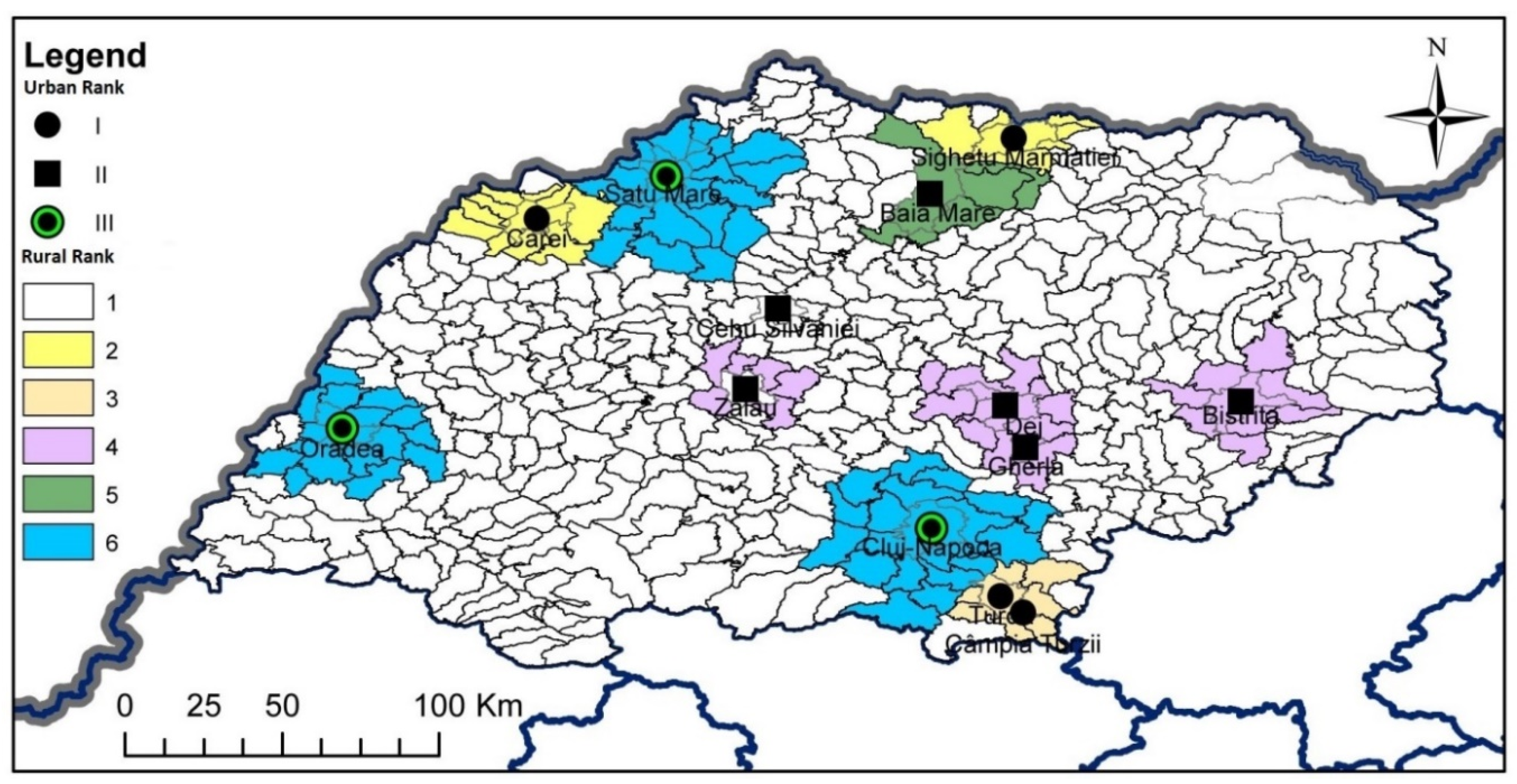
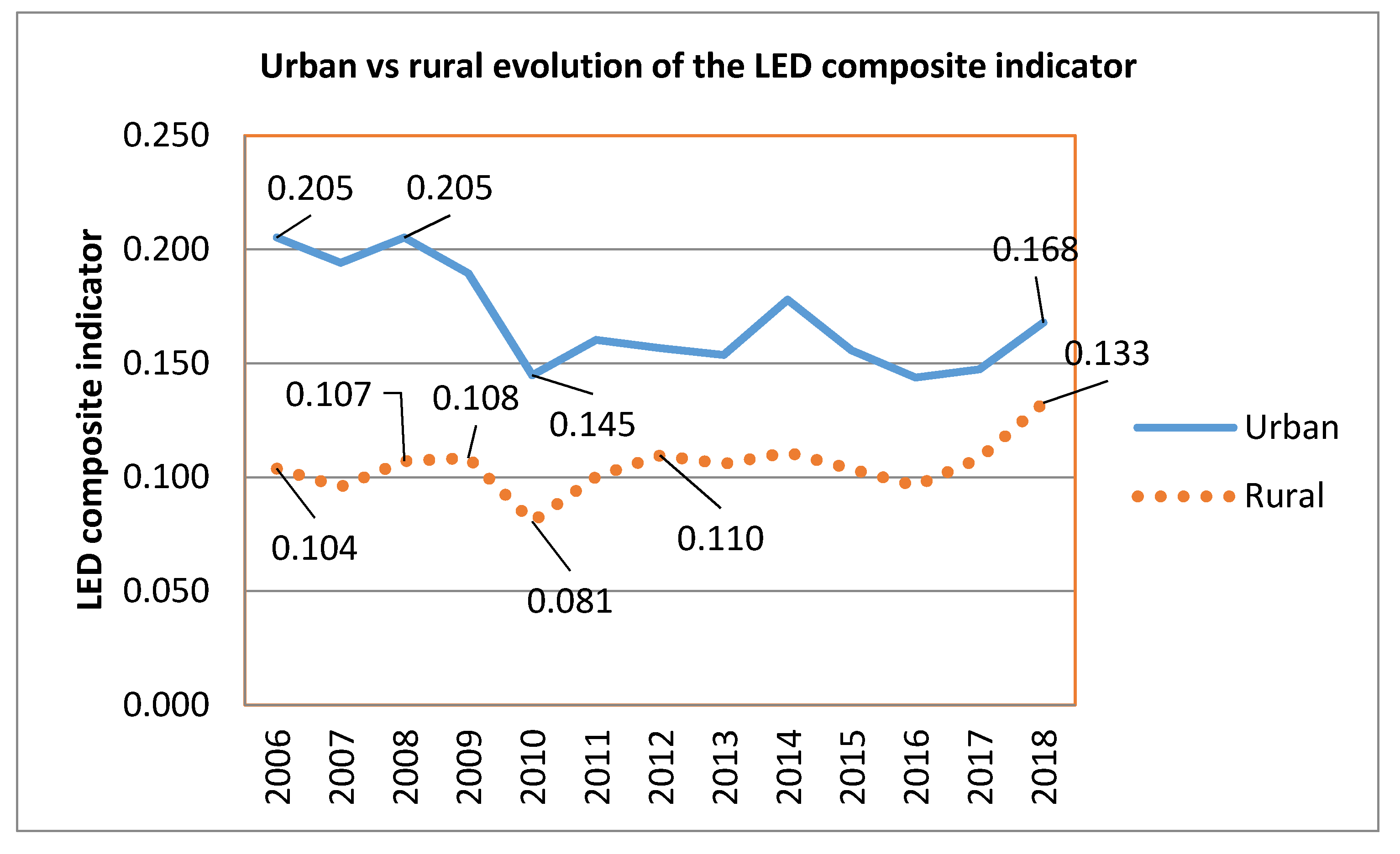
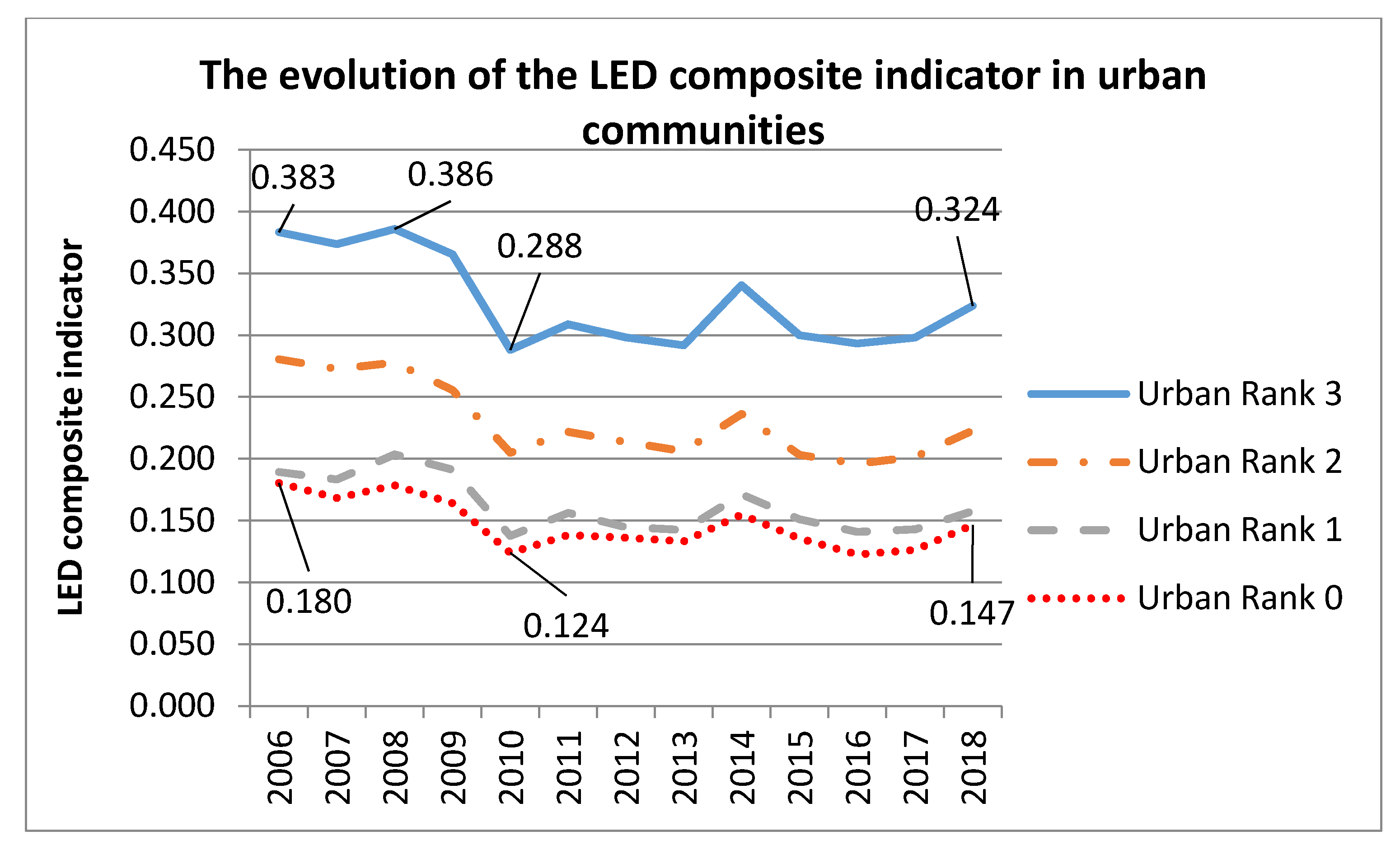
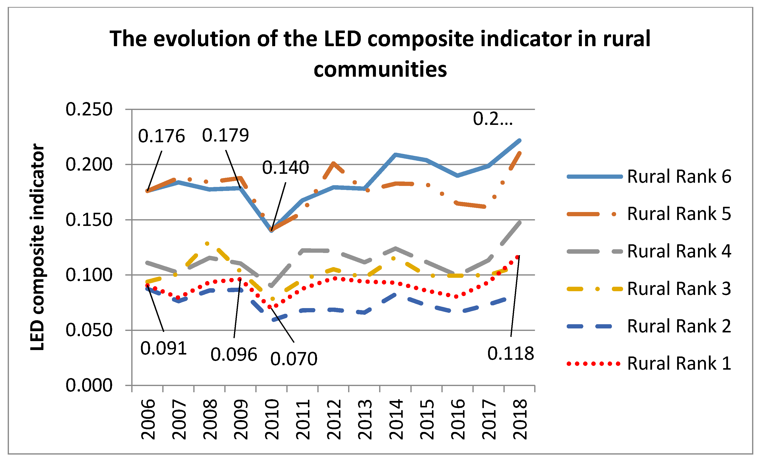
© 2020 by the authors. Licensee MDPI, Basel, Switzerland. This article is an open access article distributed under the terms and conditions of the Creative Commons Attribution (CC BY) license (http://creativecommons.org/licenses/by/4.0/).