Minimizing Shadow Area in Mountain Roads for Improving the Sustainability of Infrastructures

Abstract

The lack of sunlight on mountain roads in the wintertime leads to an increase in accidents. In this paper, a methodology is presented for the use of sunny and shady areas to be included as a parameter in road design. The inclusion of this parameter allows for the design of an iterative method for the projected infrastructures. The parameterization of the road layout facilitates the possibility of applying an iterative process of modifying the geometric elements that constitute it, examining different layout alternatives until a layout is achieved in which the surface area in the shady area is minimized, increasing the road safety and minimizing environmental impact. The methodology has been defined, generating and analyzing the results of the solar lighting study using a file in IFC format capable of integrating with the rest of the design elements (platform, signaling, structures, etc.) and thus obtaining a BIM format which allows the model to be viewed in three dimensions and moves towards 4D and 5D. The model used for the study was a high mountain road located in the province of Teruel (Spain). It is a road section characterized by successive curves in which several traffic accidents have occurred due to running off the road, partly because of the presence of ice on the platform.

1. Introduction

The mountain roads in the coldest months of the year (between November and April) withstand short periods of insolation each day. Cold temperatures with raining and snowing periods make them dangerous, with significantly increasing accident rates [1,2,3,4,5,6,7,8,9]. On very icy roads, crashes occur 16 times more often and average speeds are 17% lower than non-icy roads [10].

All this makes it necessary to establish during this winter period an operation for maintaining the roads in the best possible conditions of comfort and safety for the users and their environment. This operation is called the Winter Roads Campaign [1,10,11,12], and its tasks are aimed at avoiding the formation of ice sheets on the road and minimizing traffic disturbances as a result of snowfall, removing snow as soon as possible and avoiding blocking vehicles on the roads. These actions can be classified as preventive (avoiding ice formation) or palliative (after snowfall).

Among the substances used for ice prevention and removal, sodium chloride (NaCl) and calcium chloride (CaCl₂) are the most commonly used, and the criteria for using one or the other is determined by the minimum temperature. Sodium chloride is used at temperatures as low as −5 °C and calcium chloride is used when temperatures are even lower [13,14,15].

Although we report the benefit of the use of these products, they also have important drawbacks. Their use leads to serious damage to plants and trees up to a distance of 200 m from the treated roads [16,17,18,19,20,21,22].

In addition, when the ice is formed, machines are sometimes needed for its removal, causing a serious deterioration in the asphalt pavement.

Pavement maintenance costs were studied in the European Union in the 2000–2010 period. There was observed an economic cost of EUR 245 million per year [18]. In France, in a harsh winter (1962–1963), the maintenance and rehabilitation costs amounted to EUR 800 million [19]. Generally, it can be estimated that the cost of repairing damages caused by snow and ice is around 30% of the total maintenance cost [8]. In addition to the economic cost, the deterioration in turn leads to a decrease in road safety since the grip conditions of the car wheels (for example) are reduced. Given the problems posed using flux materials or mechanical techniques from environmental, safety, and economic perspectives, it is necessary to minimize their use. Among the most important measures, good road design stands out. Avoiding the appearance of shady areas is the most effective; by using solar energy strategically, these adverse effects decrease.

For these reasons, the geometric design of the road layout is a crucial factor, as is the study of the areas of sun and shade. There are several references for the geometric design of roads and their integration into the environment [12,23,24,25,26], but none of them have included the influence of the shadows appearing because of mountain slopes near roads. In this paper we will demonstrate the effect of design on road maintenance and safety improvement.

The development of BIM (Building Information Modeling) for the architecture, engineering, and construction industry (AEC) has facilitated accurate construction modeling, transforming 2D plans into 3D models, significantly impacting the building design lifecycle, increasing construction quality, and improving collaboration between different engineering disciplines [27]. It is necessary to incorporate the results obtained from the shadow analysis into this methodology. Insight into the results is obtained, allowing an in-depth design process in which the optimal result is manifested in the final product. In this case (and in most cases), a correct design of the linear work, paying special attention to the slope design, is the most effective prevention tool.

In the AEC industry, the development of computational design has allowed the introduction of structural elements in the modeling of linear works, including culverts, walls, bridges, tunnels, etc. [28].

2. Objectives

The purpose of this research is to define a methodology for the use of solar lighting in the design process of new roads. This methodology, applied from the design process, gives a completely new possibility for the analysis and prevention of icing points, increasing the sustainability of new infrastructures and reducing traffic accidents. The results obtained corresponding to the unlit (shaded) areas are exported to BIM format, capable of being integrated as one more element of information to the model. In this way, it is possible to increase or enrich BIM models in such a way that the choice of an optimal solution can be made. The increase in the sustainability of the infrastructure is directly related to:

−

Avoiding the discharge of anti-ice salts that cause the salinization of soils (and loss of ecosystems) as well as the contamination of groundwater.

−

Avoiding the wear of the pavement and therefore the need to repair it. Therefore, the use of bituminous material is reduced throughout the useful life of the road.

3. Methods and Material Studied

The calculation of shadows on the earth’s surface or the infrastructures projected on it can be performed in two different ways depending on whether we assume the focus (sun) as its own or improper point. If the exact position of the sun is considered (150 million kilometers away from the earth’s surface), it will give rise to a cylindrical projection, since despite being a conical projection, being so far away it approaches a cylindrical projection. If we carry out a simplification and assume the position of the sun at a distance of 10–100 km, the calculation of the surplus is approached according to a conical projection.

Reviewing the state of the art of the different software currently available, we can see a predominance of those that use the cylindrical projection; for example, AutoCAD, QGIS, ArcGIS, SAGA, GRASS [29,30,31], compared to the simplified conic. Among the latter, a software program widely used in the design of linear works stands out, such as Istram [32], which allows other calculation possibilities such as obtaining visual basins where the observer is located at a specific point; for example, a watchtower against fire.

In this research, the second method was chosen since it is specific software [32] for the design of linear works (SDOL) that allows parameterization and the creation of BIM models.

However, regardless of the projection method used, in the process of obtaining the sunny areas, it is necessary to carry out some common intermediate steps, which are described below.

3.1. Determination of the Solar Position

In both cases of cylindrical and conical projection, it is necessary to know the position of the sun. From the direction of the cylindrical projection is the radius vector Sol-study point (for example, the center of gravity of the area to be studied) and in the conical projection is the focus itself.

To determine the position of the sun, we have to obtain the azimuth angle ($\alpha )$ and the solar height angle (e).

• Solar height angle (e) is the angle between the line that joins the center of the sun with the observation point and the horizontal surface. Due to rotational and translational movements the earth makes, solar height angle varies throughout the days of the year and the hour of the day.
• Azimuth angle (α) is the angle between the horizontal projection of the line that joins the sun’s center with the local meridian.

For obtaining the azimuth and solar height, we employ the following data and equations [1,2,3,4]:

• Geographical coordinates, expressed in latitude and longitude: (φ, λ).
• Observation date (month, day), which allows the calculation of the declination δ. For calculating the declination parameter, commonly employed is the equation:

  $$\delta =23.45*sin\lceil 360*\left(\frac{284+n}{365}\right)\rceil$$

  (1)
  n = number of the day in a complete year [1 to 365].
• Observation time (H) is the horary angle, which is obtained for each hour knowing that at 12:00 p.m. the value is 0° and the sun moves 15° by the hour.

From the previous data, the azimuth angle α and the angle that determines the height above the horizon are obtained.

$$senϵ=sen\phi sen\delta +\cos \phi \cos \delta \cos H$$

(2)

$$sen\alpha =\frac{senH\cos \delta }{\cos e}$$

(3)

The transformation of the previous spherical coordinates (α, ϵ) to Cartesian is:

$$\overrightarrow{A}\left(t\right)\left(\begin{array}{c}{X}_S\\ Y_S\\ Z_S\end{array}\right)\left(t\right)=d\left(\begin{array}{c}\cos {ϵ}_S\left(t\right) \cos {\alpha }_S\left(t\right)\\ \cos {ϵ}_S\left(t\right)sen{\alpha }_S\left(t\right)\\ sen{ϵ}_S\left(t\right)\end{array}\right)$$

(4)

In summary, three key steps are necessary: (a) Determination of the earth point by geographical coordinates. (b) With (a) and the day of the year and the declination, the spherical celestial coordinates are obtained. (c) Spherical coordinates are transformed to Cartesian coordinates to be able to work on a projection.

By means of the previous equations, the position of the sun is defined, in such a way that in the case of the cylindrical projection, the radius is determined by the values (α, ϵ). However, if the problem with the conical projection is to be addressed, the earth–sun distance, d, is necessary. If we use the real value of the distance (149.6 million km), the current software programs present instabilities because of the difference in coordinates between the study point, which, in the case of a UTM-ETRS89 reference system, are 6 or 7 whole digits and three decimals, compared to 12 whole digits that represent the solar position. It is for this reason that the aim is to reduce the sun–earth distance, d.

However, the reduction of this distance d has consequences regarding the error made between the real shadow (cylindrical or conical with a distance of 146 million kilometers) and the simplified one as a consequence of this reduction.

To do this, an iterative process is proposed in which d varies between 10,000 and 100,000 m, such that the error made is less than an acceptable value. In the case of shadows affecting a road, 0.50 m can be assumed, considering the ditch plus the shoulder is more than one meter long, and so even considering the error, the shadow will never reach the rails of the road.

Defining the focus in coordinates similar to those of the reference system (ETRS89), we proceed to the calculation of shadows. For this, a beam of planes containing the Z axis is determined, separated by a certain angle determined by the precision of the results obtained, and by the distance between the area of interest and the position of the light focus (sun).

3.2. Shadow Calculation Algorithm

The calculation scheme differs considerably depending on whether one projection or another is used. In this investigation, the calculation procedure corresponding to the conical projection is developed.

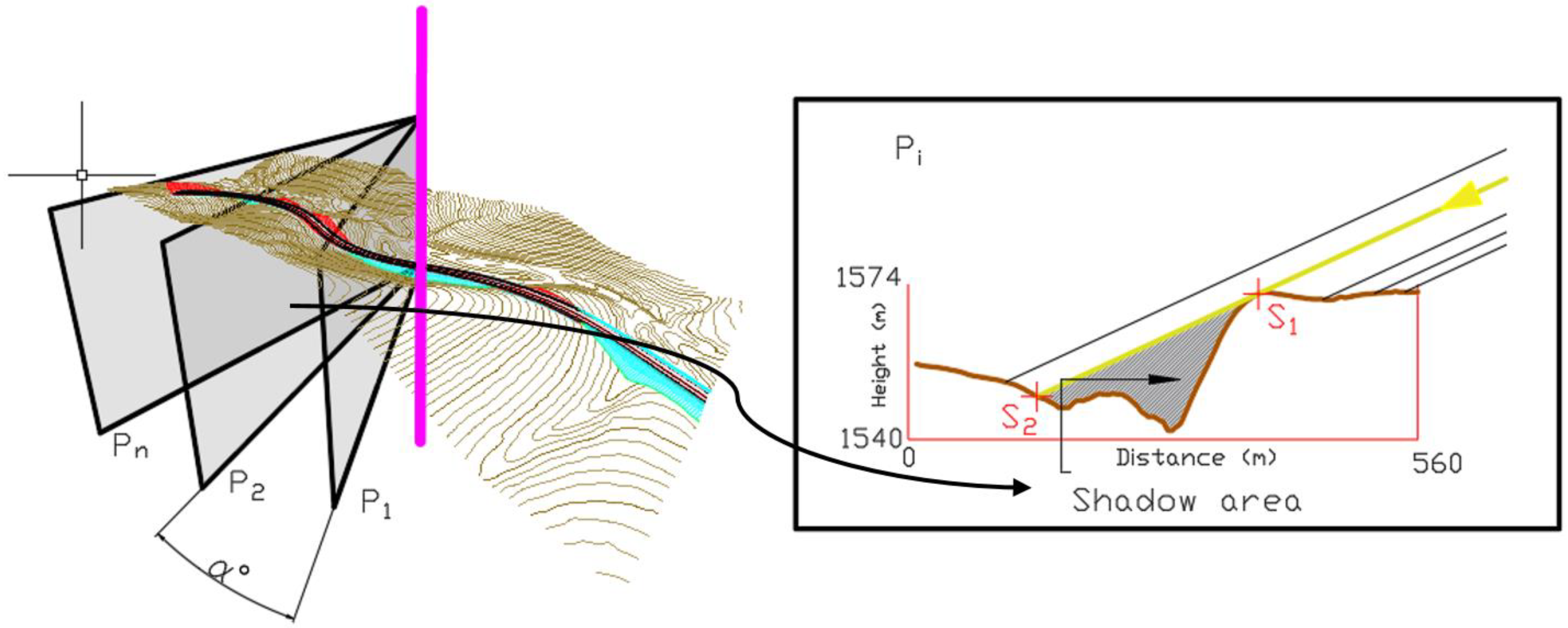
Once the position of the sun has been defined assuming a distance d, a plane beam is generated, whose common axis is the vertical straight line that contains the sun. This plane beam has an angular separation p, depending on the precision you want to obtain, as shown in Figure 1. From each of the sections obtained, P_i, you obtain a profile and a beam of lines whose origin is in focus. The shadow zone is determined by the lower part of the ray, which is tangential to the topographic surface, as shown in Figure 1. The contact point S₁ and the intersection with the terrain S₂ form part of the limit of the shadow zone. The set of points obtained from the n planes constitute the geometric place of the contour of the shaded area, as shown in Figure 2.

3.3. Parameterization of the Linear Work

The design of a linear work is carried out in three clearly differentiated phases. The first of these consists of the geometric fit of the floor plan: a succession of straight alignments and circular curves in the transition of which spirals are used, and curves characterized by a linear transition of the curvature [21]. The second phase fits the elevation layout through the succession of straight alignments linked with parabolic agreement curves (Equation (5)). Finally, in a third phase, the cross section of the road is parameterized. In summary, it can be said by means of the first two phases that a 3D traverse is obtained which satisfies geometric constraints, and in a third phase, a complex extrusion of the cross section (which is the same actual road) is materialized, which must be adapted to the topographic surface.

$$y=\frac{x^2}{2K_v}$$

(5)

The design of a linear work is an iterative process in which both the plan, elevation, and cross section are modified until a definitive layout is achieved. All this highlights the importance of the parameterization of the linear work to reduce the calculation time in the iterative process described.

Thus, it is necessary to use software that encompasses both linear work design and shadow calculation lines. Otherwise, the iterative process is considerably complicated since it involves the migration of files between both software programs. Therefore, the use of computer programs addresses the design of linear works and the study of shadows is recommended.

Once the design has been carried out, the linear work model is converted, together with the linear cartography, into a TIN (irregular network of triangles) or MDT model in which both models are perfectly integrated, as shown in Figure 3.

3.4. Export to BIM Format

Following the steps indicated in the previous sections, a set of 3D polygons are obtained corresponding to the areas where the shading conditions exist. The dimensions of this traverse are those of the land surface or the infrastructure being analyzed. To transform the 3D polyline into a surface, simply delimit the TIN that has already been generated previously; specifically, the limit is defined by the traverse. In this way, a set of surfaces is obtained that obey the shaded areas.

Next, the shaded enclosures with the TIN structure are converted into a BIM object so it can be interchangeable with the different actors that make up the construction process. There are several computer applications capable of transforming the triangulated surface into a 3D object: Istram, AutoCAD Civil 3D, etc.

Under the universal approach to collaborative design, implementation and operation of infrastructures based on workflows and open standards (open BIM), it is required for all users to export the models in the same exchange language under open standards. It is for all the above that different standards have been developed, of which in civil engineering we can highlight: IFC [33,34], OGC LandInfra (InfraGML), LandXML [35]. This research uses the IFC (Industry Foundation Classes) format, a common standard for data exchange in the construction industry that allows information to be shared regardless of the software application being used.

4. Case Study: Area Description

The stretch of road in which the methodology set out in the previous point was applied belongs to the autonomous road network of the Government of Aragon (Spain). Specifically, it is the A-226 road and the section in question is located between kilometer points (PK) 22–23, with a length of 1234.9 m, between the towns of Corbalán and Cedrillas (Figure 4).

The A-226 road (Teruel-Calanda) crosses mostly mountain areas, characterized by a winding path that crosses four mountain passes, including the Port of Cabigordo (1600 m). The towns it passes through are: Corbalán, Cedrillas, Monteagudo del Castillo, Allepuz, Villarroya de los Pinares, Fortanete, Cantavieja, and Mirambel. From there, the road ends in the Province of Teruel and continues in the Province of Castellón, renamed CV-121. After crossing the town of Olocau del Rey in Castellón, the road crosses the Province of Teruel again and is renamed A-226. In this section, it crosses the towns of Bordón, Castellote, and Mas de las Matas until reaching the town of Calanda where it joins the N-211 road. The main characteristics are indicated in

Table 1. Characteristics of the A-226 road.

A-226 (Teruel-Cantavieja)
No. of lanes	2
Lane width	3 m
Shoulder width	1 m
Maximum slope	7%
Max. superelevation	8%
Minimum radius	250 m
Parabolic curve	Concave: 3000
	Convex 2300
Allowed speed	90 km/h
Recommended speed	50 km/h
Pavement	Hot bituminous mixture

.

The section to be analyzed presents a very characteristic problem of mountain roads with high elevations—the lack of insolation—a problem that is further exacerbated by the adverse weather conditions to which it is subjected (snow and ice).

In Figure 5 it can be seen that the curve located at PK 22 + 600 is preceded by a straight line of approximately 500 m, which causes the maximum speed a vehicle with average performance can reach to be approximately 140 km/h. However, this speed is higher than the allowed (90 km/h) and recommended (50 km/h). In Figure 6, the speed diagram is shown in both.

In view of Figure 5 and Figure 6, it is observed in the increasing sense of the PKs (GOING) that it is necessary to reduce the speed (braking) at the entrance of the first curve, which causes a risk situation as a consequence of the permanence of ice or snow due to the insolation of the section in question. However, in the decreasing sense of the PKs (TURN), speed reduction is carried out at the midpoint of the straight.

Figure 7 shows the evolution of the shadow zone throughout the day corresponding to the winter solstice, 21 December. From this figure, the following conclusions can be drawn:

Until approximately 9:00 a.m., practically the entire route is in shadow.

Starting at 9:00 a.m., the first midpoint of the straight line is sunny, so the problem seen in the TURN direction is solved.

Until 11:00 h, the road remains in the shadow area near the curve where speed reduction is necessary, which suggests the presence of ice until approximately 12:00 h (

Table 2. Shaded surface of the road section between PK 21+600 and 22+800.

Hour	Winter Solstice (21 December)		Spring Equinox (21 March)		Autumn Equinox (21 September)
	Shaded Surface (m2)	% of Total (9600 m2)	Shaded Surface (m2)	% of Total (9600 m2)	Shaded Surface (m2)	% of Total (9600 m2)
8:00	9600	100%	9600	100%	9639	100%
9:00	9600	100%	3152	33%	9639	100%
10:00	4455	47%	992	10%	2673	28%
11:00	2097	22%	388	4%	99	1%
12:00	1305	14%	40	0%	0	0%
13:00	711	7%	0	0%	0	0%
14:00	720	7%	0	0%	0	0%
15:00	927	10%	0	0%	0	0%
16:00	2295	24%	0	0%	0	0%
17:00	9600	100%	684	7%	0	0%
18:00	9600	100%	1700	18%	81	1%
19:00	9600	100%	9368	98%	2169	23%
20:00	9600	100%	9600	100%	9600	100%

).

In conclusion, it can be affirmed that the curve located in the PK represents a problem from the point of view of road safety and justifies the modification of the route to avoid this problem.

5. Results and Analyses

In this section, the results of the proposed methodology are shown. Considering the need to decrease the number of hours in which the current road layout is in shadow, a new layout is designed to increase solar lighting, preferably from the first hour of the day—dawn. This fact is an important factor as seen in the proposed methodology; it reduces the accident rate, as well as the winter viability maintenance costs.

Following the steps outlined in the innovation development section, to modify the current path and make the part of the path that is currently shaded transform to become sunny, there are two alternatives or a combination of them, which are: displacement in horizontal elevation of the elevation of the current layout, as shown in Figure 8.

In this case, both displacements are chosen. On the one hand, the route moves slightly to the west and at the same time the route level rises. This step involves carrying out a series of iterations in which the plan layout and elevation are involved, as well as the modification of the geometric parameters of the cross section.

Regarding the definition of the cross section, it is worth highlighting the geology of the section analyzed, characterized by the presence of rock. This fact leads to the initial design of slopes with 1H:3V, according to the typology of the terrain—hard rock. Figure 8a shows that despite locating the road in a sunny place, the road’s slope creates a shadow in the roadway. That is why the slope has to be modified to avoid the shadows.

Because of the latter, this slope must be modified (reducing the slope) until the shadow area is reduced so that both the road and the shoulder itself remain in a sunny area. This is achieved for a 4H:1V cut slope. In Figure 9, with this new proposal for a cutting slope, the entire roadway is sunny.

In Figure 10, the cross section of the two hypotheses raised is shown. As can be seen, the difference between both sections is the right cut slope. Hypothesis 1 presents a more vertical slope, typical of rocky terrain. For Hypothesis 2, the cut slope is greater for increasing the solar ray incidence, and therefore avoids the cut slope inducing shadows on the road.

The presence of combined sun/shade situations on the road is a fact that worsens driving and therefore increases the risk of accidents more than a fully shaded situation due to the traction differential that occurs. This detail must be considered regarding the degree of precision for the results obtained. Errors, or rather a level of resolution of the model greater than 1 m, can give the result that, although a priori they are correct, once the road is built can pose a problem that is difficult and expensive to solve.

Figure 11 shows in more detail the effect of the shadow caused by a cut slope 1H:3V for all cuttings.

As already indicated, this entails modifying the cuttings to a 4H:1V criterion. In Figure 12, it can be seen that the shadow is out of the road at all times.

To end this section, the result of the BIM model is shown (Figure 13 and Figure 14) in which, in addition to the new projected layout, the shadow representation is attached. To do this, the linear work model with all its elements plus the shadow corresponding to a specific hour have been federated.

Finally, the cost of the different alternatives has been evaluated. For this, the excavation and bank measurements of both hypotheses were obtained.

Table 3. Economical study of each alternative explained.

Hypothesis	Volume New Road (m3)		Cost (EUR)		Total (EUR)
	Cut	Fill	Cut (8.5 EUR/m3)	Fill (2.1 EUR/m3)
H1 (0.3I–0.3D)	41,119.6	42,185.9	349,516.6	88,590.39	438,106.99
H2 (0.3I–4.0D)	49,486.4	42,185.9	420,634.4	88,590.39	509,224.79

shows a summary of the volumes, to which a price is applied, and the total cost obtained. As it can be seen, Hypothesis 2 is more expensive than Hypothesis 1 by EUR 71,117.80.

6. Discussion and Conclusions

The methodology presented in this work allows an approach for the calculation of shadows on the ground surface and the projected linear work for any time and day of the year. The use of such information over the design of the road should be used to reduce adverse effects that shady areas have on the infrastructure.

Further, this methodology allows the alternatives to be economically valued to generally analyze the economic costs of each of the alternatives. In this case, it is observed that Hypothesis 1 has a higher cost than Hypothesis 2, but in contrast, presents an increase of 6 h with total sunny incidence of the platform. This increase of sunny influence reduces the preventive actions to do on the road (decrease in anti-icing salts), as well as a decrease in the damage of the road (and therefore a decrease in repair actions).

The methodology proposed has been developed using a single software program, which uses the information of the linear work design, shadow calculation, and BIM model. This allows the possibility of comparing different alternatives, as well as the improvement of them by an iterative design process.

The use of a BIM format as an output of the analysis of shadows supposes a realistic representation of the designed infrastructure and allows an enrichment of the BIM model by itself.

In this work, a methodology was provided that allows for the improvement of the design of a road through a shadow analysis. The results obtained show how its application can bring benefits in terms of safety, the environment, and the management of preventive maintenance of the roads. Using the exposed methodology, we can significantly reduce the formation of ice, avoiding subsequent chemical and mechanical treatments. In this way, we generate economic savings, savings in environmental damage, and a reduction in accident rates on the roads.

In this work, a novel methodology has been provided for road design, integrated into software. This represents an advance in the techniques and processes of geometric design of linear trajectories. Furthermore, this methodology could be exported to numerous fields of civil works, improving the consistency of each project. It is essential to have tools that allow the maximum number of parameters to be analyzed from the design phase, and in this case, shadows are a fundamental element in the design of efficient and safe line layouts.