Estimation of Daily Water Table Level with Bimonthly Measurements in Restored Ombrotrophic Peatland
Abstract
1. Introduction
2. An Overview of Daily Water Table Depth Estimation Methods
2.1. Estimation Methods
2.2. General Lineal Model (GLM)
2.3. k-Nearest Neighbours (KNN)
2.4. Support Vector Machines (SVM)
2.5. Decision-Tree-Based Models: Regression Tree (TREE) and Random Forest (RF)
2.6. Adaptive Boosting (ADABOOST)
2.7. Closing Considerations About Data-Driven Methods
3. Time Series Decomposition (TSD) Method: The New Proposed Method
4. Materials and Methods
4.1. Requirements for Testing Methods
4.2. Study Area
4.3. Water Table Depth Monitoring
4.4. Bimonthly Measurements
4.5. Estimation Methods Implementation, Calibration and Validation
4.6. Data Analysis and Method Performance
4.7. Impact on a Practical Application: Sum of Daily Deficit of Water Table Depth
5. Results
5.1. Water Table Observations Statistics
5.2. Methods Performance
5.3. Impact on the Computed Daily Indicator
5.4. Selection of the Reference Well
- A reference well within the basin: One well was randomly selected per basin as the reference well and, the water table depths for the remaining five wells in the basin were re-estimated. This was done for every basin;
- A reference well within another basin: The same reference wells of the previous case were chosen, but in this case, the estimation of the daily water table depths is made over the wells of all basins. The procedure is repeated for each reference well and is identified as a run in Table 7.
5.5. Measurement Frequency
6. Discussion
6.1. TSD Method Performance Explanation
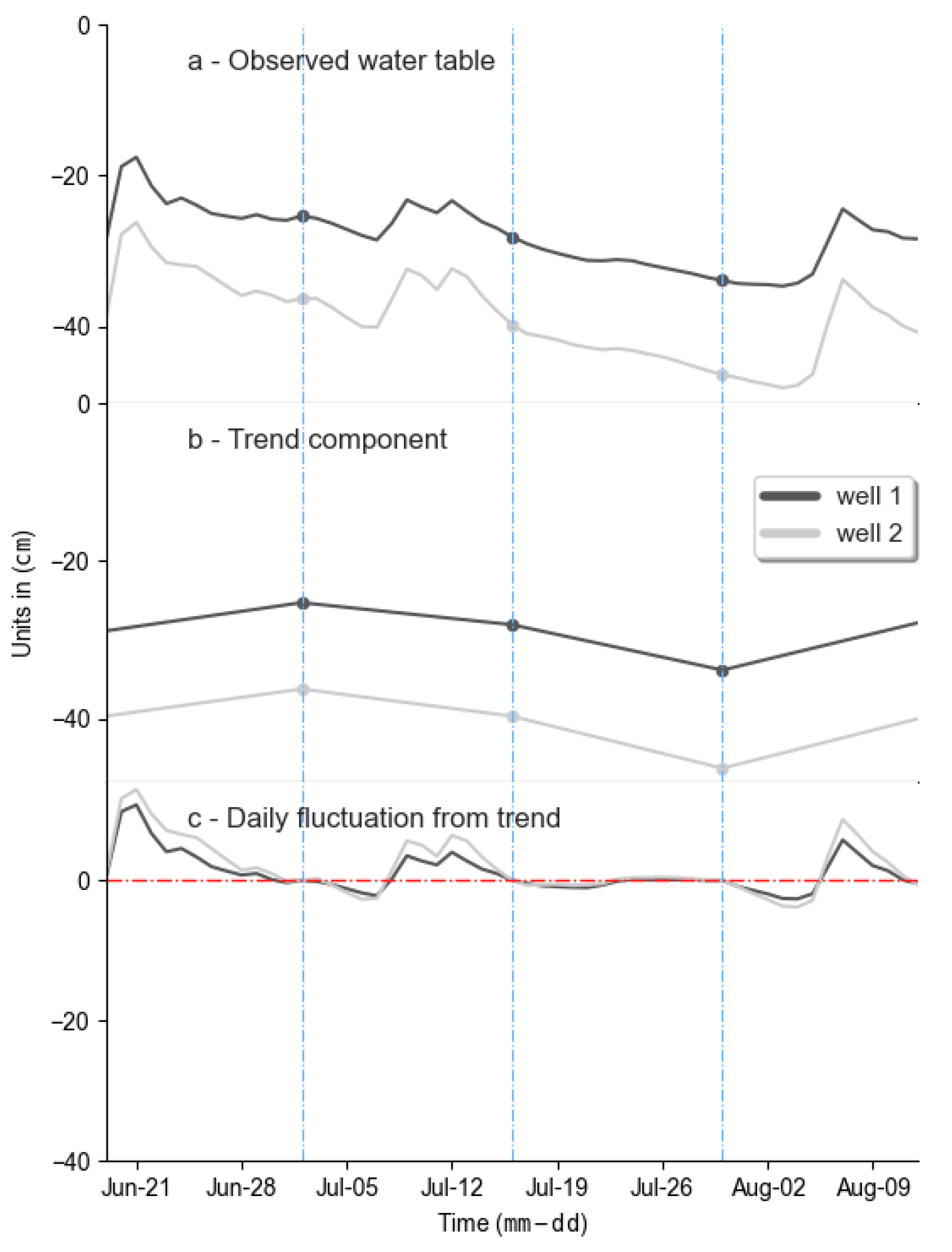
- First, TSD uses an appropriate methodological principle. It estimates the daily water table depth as the result of a local component and a regional component, which is observed in real data (Figure 1). This type of method considers regional sensitivity [80] and uses a physical concept, which is advisable [61]. Moreover, the TSD method keeps the known data (bimonthly observations) for the estimated well. The other methods generate new data, even for the observed data, which is contra-intuitive;
- Second, this method considers the time series properties, which the other methods do not consider. Time series data show auto-correlation from day-to-day data which the TSD method captures by the trend component. The other methods consider daily data as independent. Furthermore, the TSD method also captures the local impact of daily phenomena (precipitation, irrigation) through the daily fluctuation from the trend of the reference well without any additional step. Therefore, the estimated water table hydrograph is more realistic than those obtained by the remaining methods (Figure 5).
6.2. Estimation Performance by the Range of Water Table Depth Variation
6.3. Estimation of Daily Indicator
6.4. Choice of the Reference Well
7. Conclusions
Author Contributions
Funding
Institutional Review Board Statement
Informed Consent Statement
Data Availability Statement
Acknowledgments
Conflicts of Interest
Appendix A


References
- Rydin, H.; Jeglum, J. The Biology of Peatlands, 2nd ed.; Oxford University Press: Oxford, UK, 2013. [Google Scholar]
- Campbell, D.R.; Rochefort, L. La végétation: Gradients. In Écologie des tourbières du Québec-Labrador; Payette, S., Rochefort, L., Eds.; Presses de l’Université Laval: Québec, QC, Canada, 2001; pp. 129–140. [Google Scholar]
- Andersen, R.; Grasset, L.; Thormann, M.N.; Rochefort, L.; Francez, A.-J. Changes in microbial community structure and function following Sphagnum peatland restoration. Soil Biol. Biochem. 2009, 42, 291–301. [Google Scholar] [CrossRef]
- Wilson, D.; Blain, D.; Couwenberg, J.; Evans, C.D.; Murdiyarso, D.; Page, S.E.; Renou-Wilson, F.; Rieley, J.O.; Sirin, A.; Strack, M.; et al. Greenhouse gas emission factors associated with rewetting of organic soils. Mires Peat 2016, 17, 4. [Google Scholar] [CrossRef]
- Taylor, N.; Price, J.; Strack, M. Hydrological controls on productivity of regenerating Sphagnum in a cutover peatland. Ecohydrology 2016, 9, 1017–1027. [Google Scholar] [CrossRef]
- McCarter, C.P.R.; Price, J.S. The hydrology of the Bois-des-Bel bog peatland restoration: 10 years post-restoration. Ecol. Eng. 2013, 55, 73–81. [Google Scholar] [CrossRef]
- Ju, W.; Chen, J.M.; Black, T.A.; Barr, A.G.; McCaughey, H.; Roulet, N.T. Hydrological effects on carbon cycles of Canada’s forests and wetlands. Tellus Ser. B Chem. Phys. Meteorol. 2006, 58, 16–30. [Google Scholar] [CrossRef]
- Van Seters, T.E.; Price, J.S. The impact of peat harvesting nad natural regeneration on the water balance of an abandoned cutover bog, Quebec. Hydrol. Process. 2001, 15, 233–248. [Google Scholar] [CrossRef]
- Holden, J. Peatland Hydrology and Carbon Release: Why Small-Scale Process Matters. Philos. Trans. R. Soc. A-Math. Phys. Eng. Sci. 2005, 363, 2891–2913. [Google Scholar] [CrossRef]
- Brown, C.M.; Strack, M.; Price, J.S. The effects of water management on the CO2 uptake of Sphagnum moss in a reclaimed peatland. Mires Peat 2017, 20, 1–15. [Google Scholar] [CrossRef]
- Graf, M.D.; Bérubé, V.; Rochefort, L. Restoration of peatlands after peat extraction: Impacts, restoration goals, and techniques. In Restoration and Reclamation of Boreal Ecosystems; Vitt, D.H., Bhatti, J.S., Eds.; Cambridge University Press: Cambridge, UK, 2012; pp. 259–280. [Google Scholar] [CrossRef]
- Landry, J.; Rochefort, L. The Drainage of Peatlands: Impacts and Rewetting Techniques. Available online: http://www.gret-perg.ulaval.ca/uploads/tx_centrerecherche/Drainage_guide_Web_03.pdf (accessed on 13 June 2020).
- LaRose, S.; Price, J.; Rochefort, L. Rewetting of a cutover peatland: Hydrologic assessment. Wetlands 1997, 17, 416–423. [Google Scholar] [CrossRef]
- Price, J.S.; Heathwaite, A.L.; Baird, A. Hydrological processes in abandoned and restored peatlands. Wetl. Ecol. Manag. 2003, 11, 65–83. [Google Scholar] [CrossRef]
- Price, J.S. Hydrology and microclimate of a partly restored cutover bog, Quebec. Hydrol. Process. 1996, 10, 1263–1272. [Google Scholar] [CrossRef]
- Breeuwer, A.; Robroek, B.J.M.; Limpens, J.; Heijmans, M.M.P.D.; Schouten, G.C.; Berendse, F. Decreased summer water table depth affects peatland vegetation. Basic Appl. Ecol. 2009, 10, 330–339. [Google Scholar] [CrossRef]
- González, E.; Rochefort, L. Drivers of success in 53 cutover bogs restored by a moss layer transfer technique. Ecol. Eng. 2014, 68, 279–290. [Google Scholar] [CrossRef]
- Siegel, D.I.; Glaser, P. The hydrology of Peatlands. In Boreal Peatland Ecosystems; Wieder, R.K., Vitt, D.H., Eds.; Springer: Berlin/Heidelberg, Germany, 2006; pp. 289–311. [Google Scholar]
- Paradis, É.; Rochefort, L.; Langlois, M. The lagg ecotone: An integrative part of bog ecosystems in North America. Plant Ecol. 2015, 216, 999–1018. [Google Scholar] [CrossRef]
- Pellerin, S.; Lagneau, L.A.; Lavoie, M.; Larocque, M. Environmental factors explaining the vegetation patterns in a temperate peatland. C. R. Biol. 2009, 332, 720–731. [Google Scholar] [CrossRef]
- Jutras, S.; Plamondon, A.P.; Hökkä, H.; Bégin, J. Water table changes following precommercial thinning on post-harvest drained wetlands. For. Ecol. Manag. 2006, 235, 252–259. [Google Scholar] [CrossRef]
- Jutras, S.; Hökkä, H.; Bégin, J.; Plamondon, A.P. Beneficial influence of plant neighbours on tree growth in drained forested peatlands: A case study. Can. J. For. Res. 2006, 36, 2341–2350. [Google Scholar] [CrossRef]
- Price, J.S. L’hydrologie. In Écologie des tourbières du Québec-Labrador; Payette, S., Rochefort, L., Eds.; Presses de l’Université Laval: Québec, QC, Canada, 2001; pp. 141–158. [Google Scholar]
- Ireland, A.W.; Booth, R.K. Upland deforestation triggered an ecosystem state-shift in a kettle peatland. J. Ecol. 2012, 100, 586–596. [Google Scholar] [CrossRef]
- Pinceloup, N.; Poulin, M.; Brice, M.-H.; Pellerin, S. Vegetation changes in temperate ombrotrophic peatlands over a 35 year period. PLoS ONE 2020, 15, e0229146. [Google Scholar] [CrossRef]
- Holden, J.; Wallage, Z.E.; Lane, S.N.; Mcdonald, A.T. Water table dynamics in undisturbed, drained and restored blanket peat. J. Hydrol. 2011, 402, 103–114. [Google Scholar] [CrossRef]
- Haapalehto, T.; Kotiaho, J.S.; Matilainen, R.; Tahvanainen, T. The effects of long-term drainage and subsequent restoration on water table level and pore water chemistry in boreal peatlands. J. Hydrol. 2014, 519, 1492–1505. [Google Scholar] [CrossRef]
- Mioduszewski, W.; Kowalewski, Z.; Wierzba, M. Impact of peat excavation on water condition in the adjacent raised bog. J. Water Land Dev. 2013, 18, 49–57. [Google Scholar] [CrossRef]
- Waddington, J.M.; Strack, M.; Greenwood, M.J. Toward restoring the net carbon sink function of degraded peatlands: Short-term response in CO2 exchange to ecosystem-scale restoration. J. Geophys. Res. 2010, 115, 1–13. [Google Scholar] [CrossRef]
- Holden, J.; Chapman, P.J.; Labadz, J.C. Artificial drainage of peatlands: Hydrological and hydrochemical process and wetland restoration. Prog. Phys. Geogr. Earth Environ. 2004, 28, 95–123. [Google Scholar] [CrossRef]
- Taylor, N.; Price, J. Soil water dynamics and hydrophysical properties of regenerating Sphagnum layers in a cutover peatland. Hydrol. Process. 2015, 29, 3878–3892. [Google Scholar] [CrossRef]
- Price, J.S.; Whitehead, G.S. Developing hydrologic thresholds for sphagnum recolonization on an abandoned cutover bog. Wetlands 2001, 21, 32–40. [Google Scholar] [CrossRef]
- Guêné-Nanchen, M.; Pouliot, R.; Hugron, S.; Rochefort, L. Effect of repeated mowing to reduce graminoid plant cover on the moss carpet at a sphagnum farm in North America. Mires Peat 2017, 20. [Google Scholar] [CrossRef]
- Holden, J.; Swindles, G.; Raby, C.; Blundell, A. How well do testate amoebae transfer functions relate to high-resolution water-table records? In Proceedings of the EGU Geophysical Research Abstracts, Vienna, Austria, 27 April–2 May 2014; Volume 16, pp. 2014–2487. [Google Scholar]
- Parry, L.E.; Holden, J.; Chapman, P.J. Restoration of blanket peatlands. J. Environ. Manag. 2013, 133, 193–205. [Google Scholar] [CrossRef]
- Shaffer, P.W.; Cole, C.A.; Kentula, M.E.; Brooks, R.P. Effects of measurement frequency on water-level summary statistics. Wetlands 2000, 20, 148–161. [Google Scholar] [CrossRef]
- BWSR Minnesota Board of Water & Soil Resources Hydrologic Monitoring of Wetlands MN Board of Water & Soil Resources Supplemental Guidance. Available online: Ttps://bwsr.state.mn.us/sites/default/files/2018-12/WETLANDS_delin_Hydrologic_Monitoring_of_Wetlands_Guidance_BWSR.pdf (accessed on 4 August 2020).
- Pouliot, R.; Hugron, S.; Rochefort, L. Sphagnum farming: A long-term study on producing peat moss biomass sustainably. Ecol. Eng. 2014, 74, 135–147. [Google Scholar] [CrossRef]
- Hawes, M. The Hydrology of Passive and Active Restoration in Abandoned Vacuum Extracted Peatlands, Southeast Manitoba. Ph.D. Thesis, Brandon University, Brandon, MB, Canada, 2018. [Google Scholar]
- Dimitrov, D.D.; Grant, R.F.; Lafleur, P.M.; Humphreys, E.R. Modeling the Subsurface Hydrology of Mer Bleue Bog. Soil Sci. Soc. Am. J. 2010, 74, 680–694. [Google Scholar] [CrossRef]
- St-Hilaire, F.; Wu, J.; Roulet, N.T.; Frolking, S.; Lafleur, P.M.; Humphreys, E.R.; Arora, V. McGill wetland model: Evaluation of a peatland carbon simulator developed for global assessments. Biogeosciences 2010, 7, 3517–3530. [Google Scholar] [CrossRef]
- Frolking, S.; Roulet, N.T.; Moore, T.R.; Lafleur, P.M.; Bubier, J.L.; Crill, P.M. Modeling seasonal to annual carbon balance of Mer Bleue Bog, Ontario, Canada. Global Biogeochem. Cycles 2002, 16, 1030. [Google Scholar] [CrossRef]
- Daliakopoulos, I.N.; Coulibaly, P.; Tsanis, I.K. Groundwater level forecasting using artificial neural networks. J. Hydrol. 2005, 309, 229–240. [Google Scholar] [CrossRef]
- Coppola, E.; Poulton, M.; Charles, E.; Dustman, J.; Szidarovszky, F. Application of artificial neural networks to complex groundwater management problems. Nat. Resour. Res. 2003, 12, 303–320. [Google Scholar] [CrossRef]
- Taormina, R.; Chau, K.-W.; Sethi, R. Artificial neural network simulation of hourly groundwater levels in a coastal aquifer system of the Venice lagoon. Eng. Appl. Artif. Intell. 2012, 25, 1670–1676. [Google Scholar] [CrossRef]
- Mohanty, S.; Jha, M.K.; Kumar, A.; Sudheer, K.P. Artificial neural network modeling for groundwater level forecasting in a river island of eastern India. Water Resour. Manag. 2010, 24, 1845–1865. [Google Scholar] [CrossRef]
- Coulibaly, P.; Anctil, F.; Aravena, R.; Bobée, B. Artificial neural network modeling of water table depth fluctuations. Water Resour. Res. 2001, 37, 885–896. [Google Scholar] [CrossRef]
- Nayak, P.C.; Satyaji Rao, Y.R.; Sudheer, K.P. Groundwater level forecasting in a shallow aquifer using artificial neural network approach. Water Resour. Manag. 2006, 20, 77–90. [Google Scholar] [CrossRef]
- Freedman, D.A. Chapter 2. Regression Line. In Statistical Models: Theory and Practice; Freedman, D.A., Ed.; Cambridge University Press: Berkeley, CA, USA, 2009; pp. 18–28. [Google Scholar]
- Lu, W.X.; Zhao, Y.; Chu, H.B.; Yang, L.L. The analysis of groundwater levels influenced by dual factors in western Jilin Province by using time series analysis method. Appl. Water Sci. 2014, 4, 251–260. [Google Scholar] [CrossRef]
- Choubin, B.; Malekian, A. Combined gamma and M-test-based ANN and ARIMA models for groundwater fluctuation forecasting in semiarid regions. Environ. Earth Sci. 2017, 76, 1–10. [Google Scholar] [CrossRef]
- Wang, W. Stochasticity, Nonlinearity and Forecasting of Streamflow Processes; IOS Press: Amsterdam, The Netherlands, 2006. [Google Scholar]
- Cover, T.M.; Hart, P.E. Nearest Neighbor Pattern Classification. IEEE Trans. Inf. Theory 1967, 13, 21–27. [Google Scholar] [CrossRef]
- Lall, U.; Sharma, A. A Nearest Neighbor Bootstrap For Resampling Hydrologic Time Series. Water Resour. Res. 1996, 32, 679–693. [Google Scholar] [CrossRef]
- Raschka, S.; Vahid, M. Python Machine Learning. Machine Learning Deep Learning with Python, Scikit-Learn, and TensorFlow, 2nd ed.; Packt Publishing Ltd.: Brimingham, UK, 2017. [Google Scholar]
- Modaresi, F.; Araghinejad, S. A comparative assessment of support vector machines, probabilistic neural networks, and K-nearest neighbor algorithms for water quality classification. Water Resour. Manag. 2014, 28, 4095–4111. [Google Scholar] [CrossRef]
- Sakizadeh, M.; Mirzaei, R. A comparative study of performance of K-nearest neighbors and support vector machines for classification of groundwater. J. Min. Environ. 2016, 7, 149–164. [Google Scholar] [CrossRef]
- Vapnik, V.N.; Chervonenkis, A.Y. ОБ ОДНОМ КЛАССЕ АЛГОРИТМОВ ОБУЧЕНИЯ РАСПОЗНАВАНИЮ ОБРАЗОВ (A Class of Algorithms of Learning). Available online: http://www.mathnet.ru/php/archive.phtml?wshow=paper&jrnid=at&paperid=11678&option_lang=rus (accessed on 16 June 2020).
- Cortes, C.; Vapnik, V. Support-Vector Networks. Mach. Learn. 1995, 20, 273–297. [Google Scholar] [CrossRef]
- Witten, I.H.; Frank, E. Data Mining: Practical Machine Learning Tools and Techniques, 2nd ed.; Diane, C., Ed.; Morgan Kaufmann Publishers: Burlington, MA, USA, 2005. [Google Scholar] [CrossRef][Green Version]
- Zhao, T.; Zhu, Y.; Ye, M.; Mao, W.; Zhang, X.; Yang, J.; Wu, J. Machine-Learning Methods for Water Table Depth Prediction in Seasonal Freezing-Thawing Areas. Groundwater 2020, 58, 419–431. [Google Scholar] [CrossRef] [PubMed]
- Rahman, A.T.M.S.; Hosono, T.; Quilty, J.M.; Das, J.; Basak, A. Multiscale groundwater level forecasting: Coupling new machine learning approaches with wavelet transforms. Adv. Water Resour. 2020, 141, 103595. [Google Scholar] [CrossRef]
- Breiman, L.; Friedman, J.H.; Olshen, R.A.; Stone, C.J. Classification and Regression Trees; CRC Press: Belmont, CA, USA, 1984; ISBN 9781351460491. [Google Scholar] [CrossRef]
- Quinlan, J.R. Induction of decision trees. Mach. Learn. 1986, 1, 81–106. [Google Scholar] [CrossRef]
- Rokach, L.; Maimon, O. Data Mining with Decision Trees, 2nd ed.; World Scientific Publishing Co. Pte. Ltd.: Singapore, 2015. [Google Scholar]
- Rodriguez-Galiano, V.; Mendes, M.P.; Garcia-Soldado, M.J.; Chica-Olmo, M.; Ribeiro, L. Predictive modeling of groundwater nitrate pollution using Random Forest and multisource variables related to intrinsic and specific vulnerability: A case study in an agricultural setting (Southern Spain). Sci. Total Environ. 2014, 476–477, 189–206. [Google Scholar] [CrossRef]
- Ho, T.K. Random decision forests. In ICDAR ’95, Proceedings of the Third International Conference on Document Analysis and Recognition, Montreal, QC, Canada, 14–15 August 1995; IEEE Computer Society: Washington, DC, USA, 1995; Volume 1, pp. 278–282. [Google Scholar] [CrossRef]
- Biau, G.; Scornet, E. A random forest guided tour. Test 2016, 25, 197–227. [Google Scholar] [CrossRef]
- Tyralis, H.; Papacharalampous, G. Variable Selection in Time Series Forecasting Using Random Forests. Algorithms 2017, 10, 114. [Google Scholar] [CrossRef]
- Amaranto, A.; Munoz-Arriola, F.; Corzo, G.; Solomatine, D.P.; Meyer, G. Semi-seasonal groundwater forecast using multiple data-driven models in an irrigated cropland. J. Hydroinform. 2018, 20, 1227–1246. [Google Scholar] [CrossRef]
- Koch, J.; Berger, H.; Henriksen, H.J.; Sonnenborg, T.O. Modelling of the shallow water table at high spatial resolution using random forests. Hydrol. Earth Syst. Sci. 2019, 23, 4603–4619. [Google Scholar] [CrossRef]
- Brédy, J.; Gallichand, J.; Celicourt, P.; Gumiere, S.J. Water table depth forecasting in cranberry fields using two decision-tree-modeling approaches. Agric. Water Manag. 2020, 233, 106090. [Google Scholar] [CrossRef]
- Schapire, R.E. The Strength of Weak Learnability. Mach. Learn. 1990, 5, 197–227. [Google Scholar] [CrossRef]
- Freund, Y.; Schapire, R.E. Experiments with a new boosting algorithm. In Machine Learning, Proceedings of the Thurteenth International Conference, Bari, Italy, 3–6 July 1996; Morgan Kaufmann: Burlington, MA, USA, 1996; pp. 149–156. [Google Scholar]
- Kégl, B. The return of AdaBoost.MH: Multi-class Hamming trees. In Proceedings of the International Conference on Learning Representations, Banff, AB, Canada, 14–16 April 2014. [Google Scholar]
- Xiao, T.; Zhu, J.; Liu, T. Bagging and Boosting statistical machine translation systems. Artif. Intell. 2013, 195, 496–527. [Google Scholar] [CrossRef]
- Albon, C. Adaboost Classifier. Available online: https://chrisalbon.com/machine_learning/trees_and_forests/adaboost_classifier/ (accessed on 17 June 2020).
- Zanotti, C.; Rotiroti, M.; Sterlacchini, S.; Cappellini, G.; Fumagalli, L.; Stefania, G.A.; Nannucci, M.S.; Leoni, B.; Bonomi, T. Choosing between linear and nonlinear models and avoiding overfitting for short and long term groundwater level forecasting in a linear system. J. Hydrol. 2019, 578, 124015. [Google Scholar] [CrossRef]
- Amaranto, A.; Pianosi, F.; Solomatine, D.; Corzo, G.; Muñoz-Arriola, F. Sensitivity analysis of data-driven groundwater forecasts to hydroclimatic controls in irrigated croplands. J. Hydrol. 2020, 587, 124957. [Google Scholar] [CrossRef]
- Corzo, G.; Solomatine, D. Baseflow separation techniques for modular artificial neural network modelling in flow forecasting. Hydrol. Sci. J. 2007, 52, 491–507. [Google Scholar] [CrossRef]
- Hyndman, R.J.; Athanasopoulos, G. Forecasting: Principles and Practice, 2nd ed.; OTexts: Melbourne, Australia, 2018; Available online: https://otexts.com/fpp2/ (accessed on 21 June 2020).
- Ginzburg, I.F. Discrete and continuous description of physical phenomena. J. Phys. Conf. Ser. 2017, 873, 012046. [Google Scholar] [CrossRef]
- Rochefort, L.; Quinty, F.; Campeau, S.; Johnson, K.; Malterer, T. North American approach to the restoration of wetlands. Wetl. Ecol. Manag. 2003, 11, 3–20. [Google Scholar] [CrossRef]
- Van Rossum, G.; Drake, F.L. Python 3 Reference Manual; CreateSpace: Scotts Valley, CA, USA, 2009; ISBN 10.5555/1593511. [Google Scholar]
- Oliphant, T.E. Guide to NumPy; Massachusetts Institute of Technology: Cambridge, MA, USA, 2006. [Google Scholar]
- McKinney, W. Data structures for statistical computing in Python. In Proceedings of the 9th Python in Science Conference (SciPy 2010), Austin, TX, USA, 28 June–3 July 2010; van der Walt, S., Millman, J., Eds.; pp. 56–61. [Google Scholar] [CrossRef]
- Seabold, S.; Perktold, J. Statsmodels: Econometric and statistical modeling with Python. In Proceedings of the 9th Python in Science Conference, Austin, TX, USA, 28 June–3 July 2010; pp. 92–96. [Google Scholar] [CrossRef]
- Pedregosa, F.; Varoquaux, G.; Gramfort, A.; Michel, V.; Thirion, B.; Grisel, O.; Blondel, M.; Prettenhofer, P.; Weiss, R.; Dubourg, V.; et al. Scikit-learn: Machine learning in Python. J. Mach. Learn. Res. 2011, 12, 2825–2830. [Google Scholar]
- Virtanen, P.; Gommers, R.; Oliphant, T.E.; Haberland, M.; Reddy, T.; Cournapeau, D.; Burovski, E.; Peterson, P.; Weckesser, W.; Bright, J.; et al. SciPy 1.0: Fundamental algorithms for scientific computing in Python. Nat. Methods 2020, 17, 261–272. [Google Scholar] [CrossRef]
- Lagacé, R. Chapitre 12. Calcul de l’erreur. Available online: http://www.grr.ulaval.ca/gaa_7003/index.html (accessed on 20 June 2020).


| Basin ID | Chanel Configuration | Target Water Table Depth (cm) |
|---|---|---|
| PC-NI | Peripheral, non-irrigated | None |
| CC-20 | Central | 20 |
| CC-10 | Central | 10 |
| PC-20 | Peripheral | 20 |
| PC-10 | Peripheral | 10 |
| Method | Hyperparameters of the Method | Estimated Parameters for Regression | k |
|---|---|---|---|
| TSD | No training | 0 | 0 |
| GLM | No special consideration | 2 | a1, b1 |
| SVM | degree of the polynomial function = 1 linear kernel gamma coefficient automatic | 2 | w2, b2 |
| RF | random state equals zero n_estimators = 2 max depth of the tree = 2 | 2 | f1, e |
| KNN | n_neighbours = 1 weights based in distance | 2 | f1, e |
| ADABOOST | random state equals zero n_estimators = 1 | 2 | f1, e |
| TREE | split criteria set by default random state equals zero max depth = 2 min_samples_leaf = 0.3 | 2 | f1, e |
| Basin ID | N Obs | N Wells | Mean 1 | SD | Min | Max 2 |
|---|---|---|---|---|---|---|
| 2016 | ||||||
| PC-NI | 151 | 6 | 25.33 d | 11.06 | 54.25 | 0.1 |
| CC-20 | 151 | 6 | 21.14 c | 7.6 | 40.05 | −0.6 |
| CC-10 | 151 | 6 | 12.52 b | 6.94 | 34.3 | −1.85 |
| PC-20 | 151 | 6 | 24.44 d | 8.66 | 44.55 | 2.25 |
| PC-10 | 151 | 6 | 9.34 a | 4.75 | 25.3 | −3.5 |
| 2017 | ||||||
| PC-NI | 151 | 6 | 26.9 d | 12.48 | 51.6 | −1.4 |
| CC-20 | 151 | 6 | 21.39 c | 7.45 | 44.4 | −0.45 |
| CC-10 | 151 | 6 | 11.73 b | 6.27 | 35.4 | −0.5 |
| PC-20 | 151 | 6 | 24.99 d | 8.24 | 43.05 | −1.4 |
| PC-10 | 151 | 6 | 5.43 a | 3.3 | 21.25 | −1.4 |
| Performance Criteria | Methods | ||||||
|---|---|---|---|---|---|---|---|
| TSD | GLM | SVM | RF | KNN | ADABOOST | TREE | |
| R2 | 0.95 | 0.92 | 0.91 | 0.88 | 0.88 | 0.86 | 0.82 |
| RMSE (cm) | 2.48 | 3.10 | 3.24 | 3.84 | 3.87 | 4.19 | 4.68 |
| NS | 0.95 | 0.92 | 0.91 | 0.88 | 0.87 | 0.85 | 0.82 |
| AIC | 7628 | 10,241 | 10,659 | 12,202 | 12,257 | 12,983 | 13,989 |
| Basin ID | 2016 | 2017 |
|---|---|---|
| PC-NI | 1729 b (1299–2158) | 1991 b (1552–2430) |
| CC-20 | 1065 ab (803–1326) | 1107 ab (644–1573) |
| CC-10 | 261 a (0–531) | 216 a (0–467) |
| PC-20 | 1495 b (1008–1983) | 1582 b (1142–2021) |
| PC-10 | 23 a (0–51) | 1 a (0–3) |
| Performance Criteria | Methods | ||||||
|---|---|---|---|---|---|---|---|
| TSD | GLM | SVM | RF | KNN | ADABOOST | TREE | |
| R2 | 0.98 | 0.95 | 0.94 | 0.95 | 0.96 | 0.89 | 0.95 |
| RMSE (cm·days) | 131 | 200 | 215 | 198 | 182 | 377 | 201 |
| NS | 0.98 | 0.95 | 0.94 | 0.95 | 0.96 | 0.87 | 0.95 |
| Basin ID | Nearest Well | Within the Basin | In Another Basin | ||||
|---|---|---|---|---|---|---|---|
| Run 1 | Run 2 | Run 3 | Run 4 | Run 5 | |||
| PC-NI 1 | CC-20 1 | CC-10 1 | PC-20 1 | PC-10 1 | |||
| PC-NI | 3.38 | 3.29 | - | 3.89 | 3.41 | 2.99 | 3.47 |
| CC-20 | 2.71 | 3.97 | 3.76 | - | 2.68 | 2.92 | 2.94 |
| CC-10 | 1.78 | 2.29 | 4.47 | 4.50 | - | 3.26 | 1.83 |
| PC-20 | 2.85 | 2.36 | 3.34 | 3.40 | 3.01 | - | 2.98 |
| PC-10 | 1.10 | 0.97 | 4.52 | 4.45 | 2.52 | 3.21 | - |
| Aggregated | 2.48 | 2.77 | 3.45 | ||||
| Measurement Frequency | Performance Criteria | ||
|---|---|---|---|
| R2 | RMSE (cm) | NS | |
| Weekly | 0.96 | 2.08 | 0.96 |
| Bimonthly | 0.95 | 2.48 | 0.95 |
| Monthly | 0.94 | 2.80 | 0.93 |
Publisher’s Note: MDPI stays neutral with regard to jurisdictional claims in published maps and institutional affiliations. |
© 2021 by the authors. Licensee MDPI, Basel, Switzerland. This article is an open access article distributed under the terms and conditions of the Creative Commons Attribution (CC BY) license (https://creativecommons.org/licenses/by/4.0/).
Share and Cite
Gutierrez Pacheco, S.; Lagacé, R.; Hugron, S.; Godbout, S.; Rochefort, L. Estimation of Daily Water Table Level with Bimonthly Measurements in Restored Ombrotrophic Peatland. Sustainability 2021, 13, 5474. https://doi.org/10.3390/su13105474
Gutierrez Pacheco S, Lagacé R, Hugron S, Godbout S, Rochefort L. Estimation of Daily Water Table Level with Bimonthly Measurements in Restored Ombrotrophic Peatland. Sustainability. 2021; 13(10):5474. https://doi.org/10.3390/su13105474
Chicago/Turabian StyleGutierrez Pacheco, Sebastian, Robert Lagacé, Sandrine Hugron, Stéphane Godbout, and Line Rochefort. 2021. "Estimation of Daily Water Table Level with Bimonthly Measurements in Restored Ombrotrophic Peatland" Sustainability 13, no. 10: 5474. https://doi.org/10.3390/su13105474
APA StyleGutierrez Pacheco, S., Lagacé, R., Hugron, S., Godbout, S., & Rochefort, L. (2021). Estimation of Daily Water Table Level with Bimonthly Measurements in Restored Ombrotrophic Peatland. Sustainability, 13(10), 5474. https://doi.org/10.3390/su13105474


