SMAP Soil Moisture Product Assessment over Wales, U.K., Using Observations from the WSMN Ground Monitoring Network

Abstract

Soil moisture (SM) is the primary variable regulating the soil temperature (ST) differences between daytime and night-time, providing protection to crop rooting systems against sharp and sudden changes. It also has a number of practical applications in a range of disciplines. This study presents an approach to incorporating the effect of ST for the accurate estimation of SM using Earth Observation (EO) data from NASA’s SMAP sensor, one of the most sophisticated satellites currently in orbit. Linear regression analysis was carried out between the SMAP-retrieved SM and ground-measured SM. Subsequently, SMAP-derived ST was incorporated with SMAP-derived SM in multiple regression analysis to improve the SM retrieval accuracy. The ability of the proposed method to estimate SM under different seasonal conditions for the year 2016 was evaluated using ground observations from the Wales Soil Moisture Network (WSMN), located in Wales, United Kingdom, as a reference. Results showed reduced retrieval accuracy of SM between the SMAP and ground measurements. The R² between the SMAP SM and ground-observed data from WSMN was found to be 0.247, 0.183, and 0.490 for annual, growing and non-growing seasons, respectively. The values of RMSE between SMAP SM and WSMN observed SM are reported as 0.080 m³m⁻³, 0.078 m³m⁻³ and 0.010 m³m⁻³, with almost zero bias values for annual, growing and non-growing seasons, respectively. Implementation of the proposed scheme resulted in a noticeable improvement in SSM prediction in both R² (0.558, 0.440 and 0.613) and RMSE (0.045 m³m⁻³, 0.041 m³m⁻³ and 0.007 m³m⁻³), with almost zero bias values for annual, growing and non-growing seasons, respectively. The proposed algorithm retrieval accuracy was closely matched with the SMAP target accuracy 0.04 m³m⁻³. In overall, use of the new methodology was found to help reducing the SM difference between SMAP and ground-measured SM, using only satellite data. This can provide important assistance in improving cases where the SMAP product can be used in practical and research applications.

1. Introduction

Soil moisture, particularly surface soil moisture (SSM), is a very important environmental parameter playing a key role in a number of physical processes in the Earth system, including water and carbon cycles, affecting the climate directly or indirectly [1]. It has long been recognized as a key state variable of the global energy and water cycle due to its control on exchanges of energy and matter and physical processes; in particular, the partitioning of available energy at the Earth’s surface into latent (LE) and sensible (H) heat exchange [2,3]. In addition, it can inform sustainable water resource management, the study of ecosystems and ecological processes [4,5], plant water requirements, and plant growth and productivity [6,7,8]. SSM is an important parameter in various studies, such as disaster events (drought, flood), along with agricultural productivity, water resource management, and the development of a circulation climate model at the global and regional scale. It also supports decision-making policies at the national level [9,10]. Information on SSM is essential for crop yielding and plays a vital role in food security at the global level [11,12]. The largest freshwater consumption is applied globally in the irrigation of crops [13]. About 80% of freshwater is used in irrigation by developing countries [14]. The demand for water for irrigation is increasing due to global climate change, with greater variation in annual precipitation volumes [15,16]. Accurate information about surface soil moisture is very useful for developing a sustainable agricultural irrigation system.

Despite its high importance, the large spatial and temporal heterogeneity of SSM makes it a difficult parameter to measure on a routine basis over large areas [5,17]. There are several methods available for the measurement of soil moisture using ground instrumentation, such as probes or gravimetric measurements. A comprehensive overview of the conventional methods can be found in [18]. However, point-based measurement of soil moisture may not be very useful for large scale applications because the distribution of soil moisture is highly variable, both spatially and temporally [19]. This is mainly due to the constraint of the effort and cost of setting up suitable ground networks at the required spatial and temporal scales to provide the information needed for research and operational purposes [20]. Earth Observation (EO) provides the best alternative to ground observations in deriving SSM over large regions and different geographical scales [21,22]. A recent overview of the relevant operational products available can be found in [23].

However, estimation of soil moisture by EO sensors has always been a challenge due to the presence of vegetation cover, surface roughness, variation in surface temperature and evapotranspiration. In this aspect, many studies stated that the fusion of microwave (MW) and optical remote sensing techniques may be useful for accurate estimation of the soil moisture of natural ground surfaces. In recent years, there have been several satellites available in orbit, providing data suitable for the development of global soil moisture products. These include Soil Moisture Active Passive (SMAP), Soil Moisture and Ocean Salinity (SMOS), Japan Aerospace Exploration Agency (JAXA), Advanced Microwave Scanning Radiometer, European Space Agency (ESA), Climate Change Initiative (CCI), L3 soil moisture product, and Fengyun-3B (FY3B) L2 soil moisture product [24,25,26,27]. The use of those operational products requires an extensive evaluation of their accuracy in different ecosystems, environmental conditions, and climatic zones. To this end, the presence and maintenance of operational ground monitoring networks is very important [28,29].

Evaluating the accuracy of SSM by operational products has been the focus of many studies by researchers worldwide [5,30,31]. In most of these studies, ground measurements from validated observational networks have been used as reference data against which satellite-derived SSM predictions were compared. For example, Srivastava et al. [9] investigated the SMOS satellite-derived soil moisture at a catchment scale for hydrological applications. Srivastava et al. [32] have presented the performance of the global Weather Research and Forecasting (WRF) model and the European Centre for Medium-Range Weather Forecasts (ECMWF)in relation to Noah Land surface model data for hydrological applications. They evaluated the efficiency of WRF-simulated SM for the estimation of soil moisture deficit (SMD) and compared it with SMOS downscaled and non-downscaled soil moisture. Some studies also attempted to improve rainfall runoff models by assimilating soil moisture data into hydrological or meteorological models to test their reliability at different scales and over different regions [33]. Similarly, Riechle and Koster [34] showed that surface soil moisture from the Microwave Radiometer can improve the output of NASA Catchment land surface model. Srivastava et al. [35] provided a detailed evaluation of land surface models and satellite soil moisture from Soil Moisture and Ocean Salinity (SMOS) through data fusion for improved predictions of catchment-based soil moisture deficit (SMD). Similarly, another study by Srivastava et al. [36] showed the performance of several machine learning algorithms for the prediction of catchment SMD using SMOS and land surface temperature derived from the Moderate Resolution Imaging Spectroradiometer (MODIS) with improved performance for SMD estimation during validation.

Petropoulos et al. [30] evaluated the SMOS soil moisture product accuracy using in situ soil moisture observed by the REMEDHUS International Soil Moisture Network (ISMN) at different influencing parameters, including seasonality and radio frequency. The highest accuracy of SMOS soil moisture was achieved in the autumn season followed by summer, winter, and spring seasons, and reduced the radio frequency interference (RFI) effect by filtering out the high RFI fraction. Petropoulos et al. [31] assessed the accuracy of the SMOS global operational product of soil moisture for different seasons and land cover patterns. Validation was performed with the in situ observations taken by the CarboEurope ground observational network. They also evaluated the land cover, seasonality, and RFI effect on SMOS product.

The National Aeronautics and Space Administration (NASA) launched the Soil Moisture Active Passive (SMAP) satellite on 31 January 2015. SMAP consists of L-band active (radar) and passive (radiometer) microwave instruments [34]. It provides the daily global SSM with a depth of 0–5 cm at 10 km and 40 km spatial resolution. Colliander et al. [37] selected the core 34 validation sites for the SMAP SSM product validation. Authors have reported an RMSE between observed SM and SMAP radiometer-based SM, observed SM and radar-based SM, and observed SM and combined radar–radiometer SM of 0.04 m³m⁻³, 0.06 m³m⁻³, 0.04 m³m⁻³, respectively. Chan et al. [38] enhanced the spatial resolution of SMAP passive SM product from 36km to 9km by the Backus–Gilbert optimal interpolation technique using antenna temperature (Ta) data in original SMAP Level 1B Brightness Temperature. The enhanced brightness temperature was used as a baseline for the SM retrieval algorithm. The enhanced SM was compared with in situ data for different seasons and biomes. RMSE, correlation coefficient and bias were found to be 0.040 m³m⁻³, 0.80 and −0.015 m³m⁻³ between developed enhanced SM (with 9 km grid) and soil moisture product (with 36 km grid). However, to the best of our knowledge, there are very few studies concerned so far with the evaluation of this product in an oceanic climatic zone and also outside of United States-based validation sites. This is despite the availability of suitable validated observations from global ground observational networks. A particularly useful area to perform such investigation is Wales, in the United Kingdom, because it would help understand how useful EO-based SSM products would be for a wide range of purposes, such as livestock protection, yield prediction, flood forecasting and human health. One such network providing validated observations suitable is the automated Wales Soil Moisture Network (WSMN) [28].

In purview of the above, the present study objectives are to: (1) evaluate the SM and surface temperature (ST) data using in situ measurements from WSMN and SMAP satellite data; (2) assess the effect of seasonality of SM and ST using SMAP satellite data for annual, growing and non-growing seasons; and (3) develop a model to retrieve SM using SMAP data based on multiple regression analysis, and evaluate SM prediction accuracy by this model at the WSMN.

2. Materials and Methods

2.1. Study Area and InSitu Datasets

WSMN is an in situ data network located in west Wales, U.K., covering a wide area with latitude 51.03611° to 53.65022° N and longitude −5.64258° to −1.90814° W. Wales is a mountainous country situated on the western side of central southern Great Britain. Different weather conditions are present in Wales, U.K., throughout the year, such as clouds, winters, and warm summers. The average annual temperaturesare10 °C and15 °C in winter and summer, respectively. The region on which WSMN is installed has a wide range of rock types and a variation in climate [39].

WSMN was established between 2009 and 2013 with 9 different stations near the area of Aberystwyth in Wales. WSMN currently consists of 9 stations spread across 5 sites (Figure 1) situated in the wider area of the region. A detailed description of the site characteristics composing the ground monitoring network can be found in [28]. Briefly, Sites 1 and 2 are agricultural grassland sites near to the Gogerddan campus of Aberystwyth University. Sites 3 and 4 are of bioenergy crops at the northern outskirts of Aberystwyth. Site 5 is situated under grassland of Miscanthus plots. Site 6 is situated under the willow at the eastern edge of Aberystwyth, near Llanbadarn campus of Aberystwyth. Sites 7, 8 and 9 are situated at grassland on the Pwllpeiran Research Farm, near to the Devil’s Bridges. Time domain reflectometry (TDR) has been used for the measurement of soil moisture. TDR is installed horizontally at 5–10 cm depth in the soil surface [28]. In particular, soil moisture sensor depths are 5 cm, 5 cm, 5 cm, 5 cm, 10 cm, 10 cm, 10 cm, 10 cm, and 5 cm for site 1, site 2, site 3, site 4, site 5, site 6, site 7, site 8 and site 9, respectively. A detailed description of test sites is provided in

Table 1. The detailed description of the main characteristics of the WSMN sites.

Site No.	Location/Coordinates	Established Year and Operation Duration	Site Description	Sensor Characteristics	Variables Measured
1	Comins-Coch Lat: 52.43233° N Lon: −4.02084° W	July 2013 to present	Land cover: Agriculture/Grasslands Elevation: 30 m	Sensor position: Horizontal Sensor depth: 5 cm	Soil moisture, soil temperature, vegetation water content, electrical conductivity and temperature
2	Comins-Coch Lat: 52.43244° N Lon: −4.02167° W	July 2013 to present	Agriculture/Grasslands Elevation: 28 m	Sensor position: Horizontal Sensor depth: 5 cm	Soil moisture, soil temperature, vegetation water content, electrical conductivity and temperature
3	Penglais Lat: 52.42243° N Lon: −4.06834° W	2012 to present	Land cover: Ryegrass Pastureland transitions to Miscanthus × Giganteus Bioenergy Crop Elevation: 114 m	Sensor position: Horizontal Sensor depth: 5 cm	Soil moisture, soil temperature, vegetation water content, electrical conductivity, temperature, wind speed, rainfall and relative humidity
4	Penglais Lat: 52.42146° N Lon: −4.07056° W	May 2013 to present	Land cover: Ryegrass Pastureland transitions to Miscanthus Bioenergy Crop Elevation: 110 m	Sensor position: Horizontal Sensor depth: 5 cm	Soil moisture, soil temperature, vegetation water content, electrical conductivity, temperature, wind speed, rainfall and relative humidity
5	Cae-Canol Lat: 52.41389° N Lon: −4.04278° W	2009 to present	Land cover: 16 individual plots each of willow and Miscanthus and grass rows Elevation: 128 m	Sensor position: Horizontal Sensor depth: 10 cm	Soil moisture, soil temperature, vegetation water content, electrical conductivity, and temperature
6	Cae-Canol Lat: 52.4138° N Lon: −4.04278° W	2009 to present	Land cover: 16 individual plots each of willow and Miscanthus and grass rows Elevation: 128 m	Sensor position: Horizontal Sensor depth: 10 cm	Soil moisture, soil temperature, vegetation water content, electrical conductivity, and temperature
7	Pwllpeiran Lat: 52.3653° N Lon: −3.83167° W	June 2014 to present	Land cover: Semi-Improved U4 Grassland Elevation: 375 m	Sensor position: Horizontal Sensor depth: 10 cm	Soil moisture, soil temperature, vegetation water content, electrical conductivity, temperature, wind speed, rainfall and relative humidity
8	Pwllpeiran Lat: 52.38695° N Lon: 3.75195° W	June 2014 to present	Land cover: Peatland Elevation: 500 m	Sensor position: Horizontal Sensor depth: 10 cm	Soil moisture, soil temperature, vegetation water content, electrical conductivity, temperature, wind speed, rainfall and relative humidity
9	Pwllpeiran Lat: 52.35321° N Lon: 3.80306° W	2016 to present	Land cover: Semi-Improved grassland Elevation: 260 m	Sensor position: Horizontal Sensor depth: 5 cm	Soil moisture, soil temperature, vegetation water content, electrical conductivity, temperature, wind speed, rainfall and relative humidity

.

In this study, the in situ SM and ST data were obtained by taking the averages from Comins-Coch WSMN site 1 and 2 over agriculture/grasslands land cover for the year 2016. The whole dataset was obtained from International Soil Moisture (ISMN), a global data sharing and distribution platform. The collected data were separated into the growing and non-growing seasons. The growing season starts from March to November in the United Kingdom. The non-growing season was taken as from December to February. The average yearly temperature of the non-growing season was less than 6 °C.

2.2. Satellite Datasets

SMAP provides measurements of brightness temperature at spatial resolution (~36 km) scales with a temporal resolution of 3days global coverage. The SMAP satellite is equipped with passive (radiometer) microwave instruments with the L-band (1.41 GHz). The radiometric-based algorithms provide the estimation of near-surface soil moisture (0–5 cm depth) data products. The thermodynamic temperature at the uppermost layer of the Earth’s surface is called land surface temperature (LST). It is commonly measured by the thermal radiance obtained from thermal infrared sensors over clear sky conditions [40]. The SMAP passive soil moisture product(L2_SM_P) [41,42,43] was used for extracting the temporal data of soil moisture and surface temperature for the year 2016 for WSMN soil moisture sites in the Wales, U.K. Surface temperature information was imputed to SMAP from the GMAO GEOS-5 model for the SMAP passive soil moisture algorithm. The SMAP SM and ST datasets have been downloaded from NASA Earth science data (https://earthdata.nasa.gov/) from January to December months for the year 2018. Furthermore, the 8-day composite MODIS global evapotranspiration (ET) product (MOD16A2) [44,45] with a spatial resolution of 1 km was also used in the present study to understand the changes in ET with the surface soil moisture and temperature. The aggregation process was applied to convert the ET spatial resolution of 1 km to 36 km within the SMAP pixel size. The cubic spline interpolation technique was applied to improve the temporal resolution (8 day to daily) of ET. The 16-day composite Global MODIS Aqua Vegetation Indices product (MYD13A1) was used for the extracting of normalized difference vegetation index (NDVI) data with a spatial resolution of 500 m. The ET and NDVI datasets have been downloaded from January to December months for the year 2018 (https://lpdaacsvc.cr.usgs.gov/appeears/). The mean aggregation process was applied to convert the NDVI spatial resolution 500 m to 36 km within the SMAP pixel size. The cubic spline interpolation technique was applied to improve the temporal resolution (16 days to daily) of NDVI. The Google Earth engine tool was used to extract the daily GPM rainfall data (NASA/GPM_L3/IMERG_V06). The processing of in situ and satellite datasets has been processed in open access Python libraries (pandas, numpy, matplotlib, rasterio, gdal, sklearn, and scipy) in Jupyter notebook.

2.3. Statistical Analysis

In this study, the SMAP SM and ST data were compared with the WSMN in situ data using a series of appropriate statistical metrics summarized in

Table 2. Statistical measures used to assess the agreement between the predicted estimates and the in situ observations. Subscripts i = 1. N denotes the individual observations, P denotes the predicted values, and O denotes the “observed” values. The horizontal bar denotes the mean value.

Name	Description	Mathematical Definition
Bias/MBE	Bias (accuracy) or mean average error	$bias=MBE=\frac{1}{N}{\displaystyle \sum _{i=1}^N(P_i-O_i)}$
Scatter/MSD	Scatter (precision) or mean standard deviation	$scatter=\frac{1}{(N-1)}{\displaystyle \sum _{i=1}^N{(P_i-O_i-\overline{(P_i-O_i)})}^2}$
RMSE	Root-mean-square error	$RMSE=\sqrt{bia{s}^2+scatte{r}^2}$
R2	Coefficient of determination	$R^2={(\frac{E\left[\left({\theta }_{sat}-E\left[{\theta }_{sat}\right]\right)\left({\theta }_{in-situ}-E\left[{\theta }_{in-situ}\right]\right)\right]}{{\sigma }_{sat}{\sigma }_{in-situ}})}^2$

. The coefficient of determination (R²) is the proportion of the variance in the dependent variable that is predictable from the independent variable, and it varies between 0 and 1. A higher value is an indicator of a good prediction. The bias measures the average tendency of the estimated values to be larger or smaller than their observed values. The optimum value of bias is 0.0 and the smaller value of bias indicates accurate model prediction [46]. Root-mean-square error (RMSE) is another statistical parameter frequently used to measure the differences between estimated values by a model or an estimator and the observed values [47]. The scatter or mean standard deviation shows the bias free error between observed and retrieved variables. The lower values of scatter depict good retrieval values. These specific statistical metrics were selected to be used in our study because they have also been used in many other similar studies [2,5,8,10,29,30,31].

2.4. Multiple Regression Analysis

Multiple regression analysis is a statistical procedure to establish the relationship between several independent variables and one dependent variable. The goal of multiple regression analysis is to model a dependent variable as a function of several independent variables. The independent variables may be continuous or categorical [48,49]. The estimates generated through multiple regression analysis are called coefficients. Multiple regression analysis requires at least two or more independent variables [50].

In multiple regression analysis, the relative weight age of each independent variable on the dependent variable is computed by the computation of variance in the dependent variable with respect to the variation in each of the independent variables. Mathematically, the multiple regression equation can be explained as in Equation (1),

$$Y=b_1{X}_1+b_2{X}_2+\dots \dots +b_n{X}_n+c$$

(1)

where $b_i(i=1,2,\dots ,n)$ are the regression coefficients. The values of regression coefficients show the relative importance for the changes in the dependent variable due to the changes in each independent variable with the relationship. The term c represents the y-intercept [51].

In the present study, WSMN in situ soil moisture was considered as the dependent variable, and SMAP SM and ST were considered as the independent variables for the multiple regression analysis to establish the relationship between in situ SM and satellite SM and ST for accurate retrieval.

3. Results

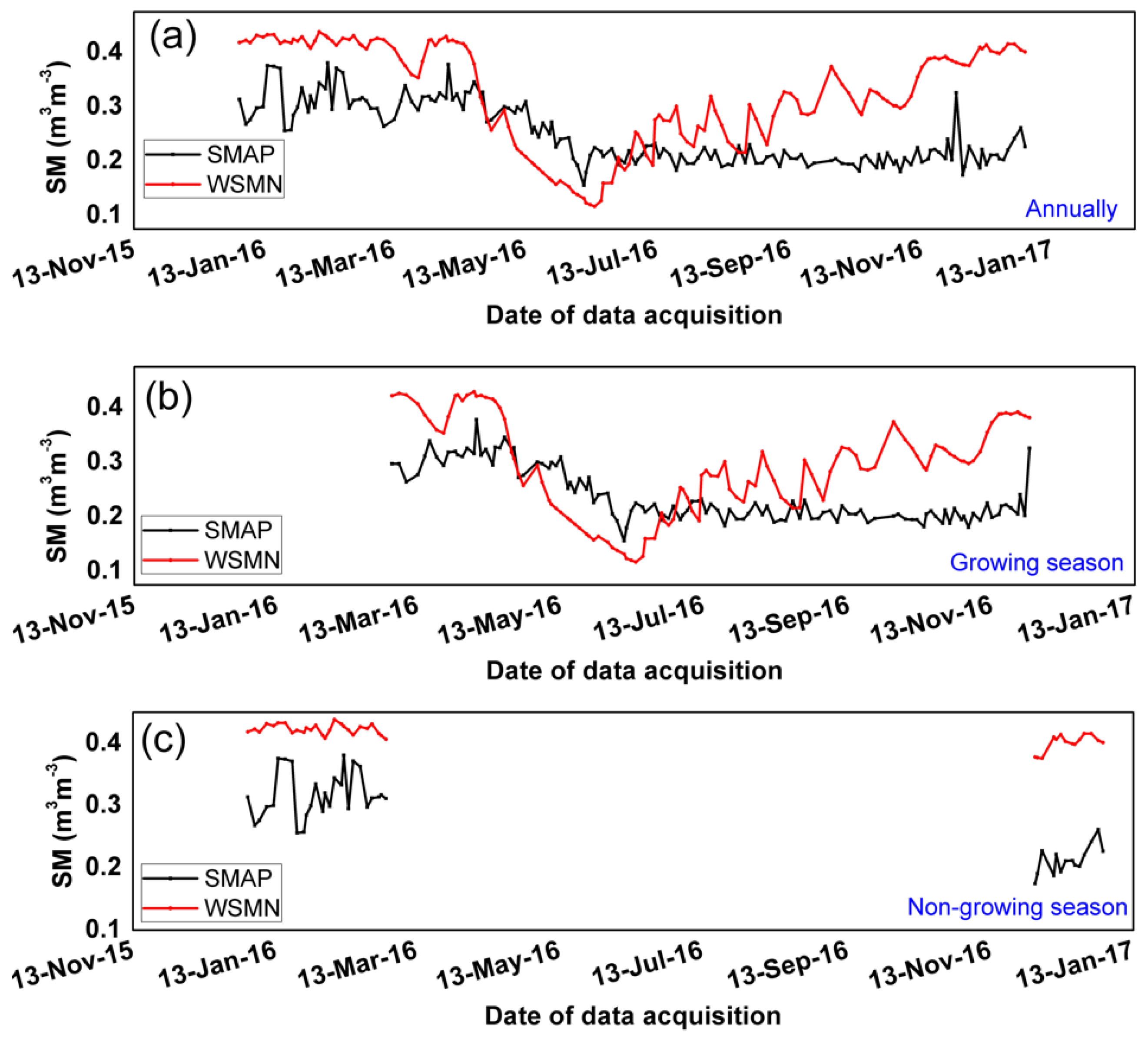
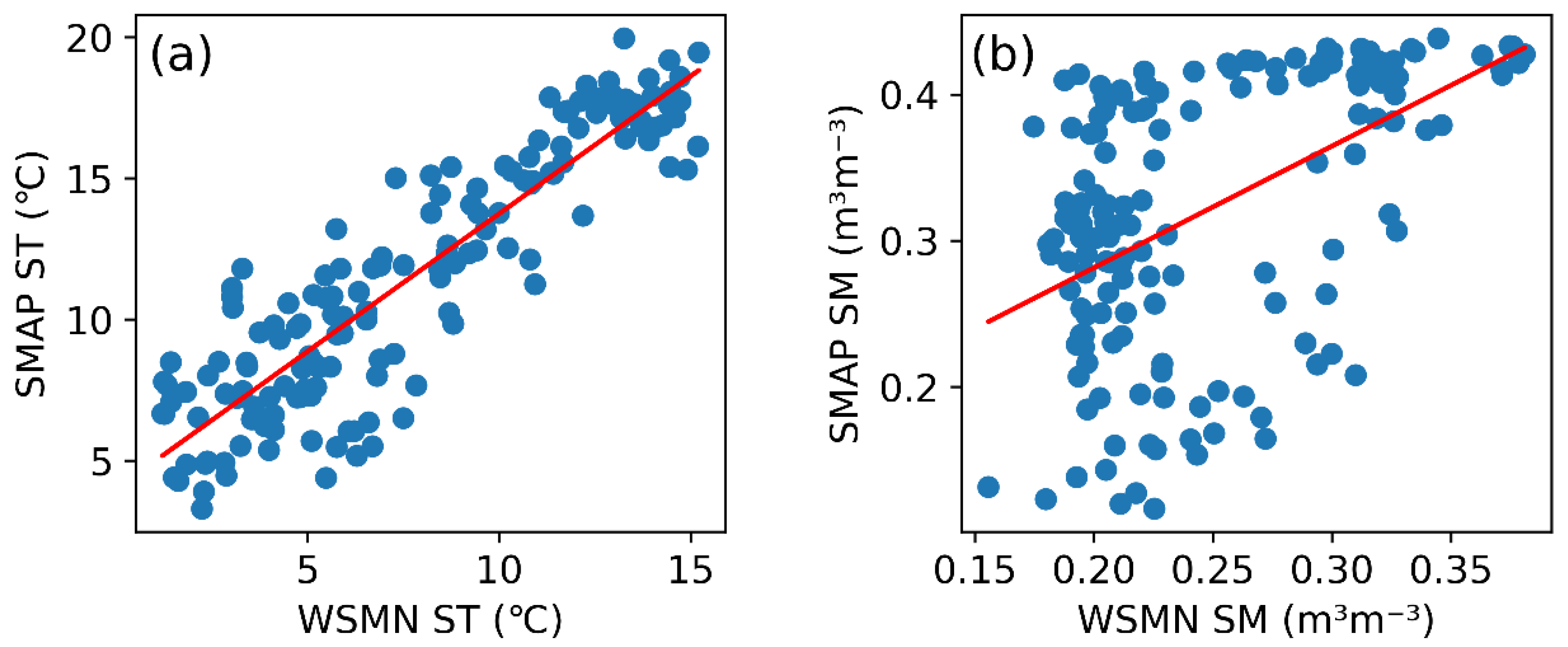
3.1. Seasonal Assessment

Figure 2a–c shows the temporal variation of the SMAP-derived SM and WSMN SM for annual, growing and non-growing seasons, respectively. A relatively poor correlation is reported between SMAP SM and WSMN SM during both annual and growing seasons with respect to non-growing seasons because the retrieval of SM was affected due to vegetation cover. Figure 3a–c shows the temporal variation of the SMAP ST and WSMN ST for annual, growing and non-growing season, respectively. Regarding the ST comparisons, SMAP and WSMN follow approximately the same pattern as each other for both the growing and non-growing seasons (Figure 3a–c). Figure 4a shows the temporal variation of SMAP SM, ST and MODIS observed ET and MODIS NDVI throughout the year 2016. Figure 4b shows the temporal variation of WSMN SM, ST and MODIS observed ET and MODIS NDVI throughout the year 2016. On the basis of Figure 4a,b, it is observed that the temporal variation of ET directly and accurately follows the temporal variation of SMAP ST and WSMN ST. The temporal variation of ET roughly inversely follows the temporal variation of SMAP SM and WSMN SM. The ET rate is more dependent on the ST than SM. The rate of change in ET follows the rate of change of ST. The SM is directly connected with the process of ET, which can be potentially evaporated from the ground surface; thus, it is clearly stated that when ET increases, SM decreases. The NDVI is a good indicator for vegetation growth. The higher value of ET is observed during the growing season because evaporation is the process of transferring water stored in the surface of canopies, stems, branches, and soil surface to the atmosphere. The soil surface loses water with the highest ΕΤ rate. The results reported herein indicate that SM, ET, and ST are correlated with each other, and variability in these parameters is due to the cumulative effect of various factors such as wind speed, humidity, precipitation, water table, drainage pattern, etc.

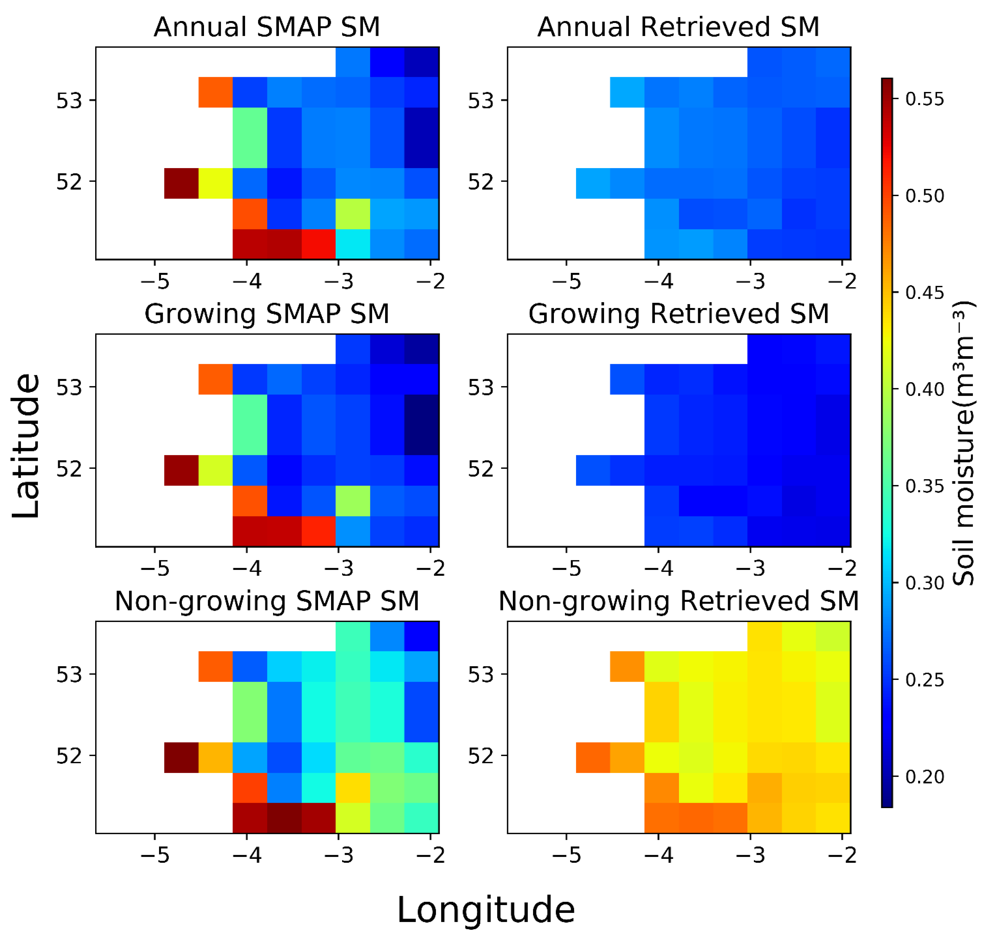
3.2. Performance Assessment of Datasets and Algorithm Development for Annual, Growing and Non-Growing Seasons

A linear regression analysis was carried out between the SMAP (SM, ST) and WSMN (SM, ST) data for annual, growing and non-growing seasons using Equation (2).

Table 3. Values of performance indices and coefficients of linear and multiple regression analysis for Equations (2) and (3).

Season	Linear Regression Analysis for SMAP (ST) and WSMN (ST) Data (Equation (2))
	R2	RMSE	Bias	Scatter/MSD	Coeff(A)	Intercept (B)		Figure No.
Annual	0.807	4.286 °C	3.803 °C	1.975 °C	0.9736	4.0092		5 (a)
Growing	0.831	4.634 °C	4.347 °C	1.604 °C	0.8546	5.6713		6 (a)
Non-growing	0.084	3.108 °C	2.278 °C	2.114 °C	0.2063	5.4880		7 (a)
Linear regression analysis for SMAP (SM) and WSMN (SM) data (Equation (2))
Annual	0.247	0.109 m3m−3	0.073 m3m−3	0.081 m3m−3	0.8321	0.1149		5 (b)
Growing	0.183	0.094 m3m−3	0.051 m3m−3	0.079 m3m−3	0.7503	0.1109		6 (b)
Non-growing	0.490	0.142 m3m−3	0.133 m3m−3	0.049 m3m−3	0.1729	0.3663		7 (b)
Multiple regression analysis for the estimation of SM (Equation (3))
Annual	R2	RMSE	Bias	Scatter/MSD	Coeff(C)	Coeff(D)	Intercept (E)	Figure No.
	0.558	0.045 m3m−3	2.135 × 10−17 m3m−3	0.045 m3m−3	0.1229	−0.0156	0.4138	8(a)
Growing	0.440	0.042 m3m−3	−3.789 × 10−17 m3m−3	0.042 m3m−3	0.1048	−0.0139	0.3915	8(b)
Non-growing	0.613	0.007 m3m−3	−5.686 × 10−17 m3m−3	0.007 m3m−3	0.2133	0.0027	0.3436	8(c)

shows the value of linear regression coefficients and performance indices (reported in Table 2) between the SMAP (SM or ST) and WSMN (SM or ST) data for annual, growing and non-growing seasons. Figure 5a,b shows the scatter plots between WSMN ST and SMAP ST and WSMN SM and SMAP SM for the annual datasets, respectively. Figure 6a,b shows the scatterplots between WSMN ST and SMAP ST and WSMN SM and SMAP SM for the growing season datasets, respectively. Figure 7a,b depicts the scatterplots between WSMN ST and SMAP ST and WSMN SM and SMAP SM for the non-growing season datasets, respectively. The values of coefficient of determination (R²) between SMAP SM and WSMN SM were found to be0.247, 0.183, and 0.490 for annual, growing and non-growing seasons, respectively. However, the values of scatter between SMAP SM and WSMN SM were found to be 0.081 m³m⁻³, 0.079 m³m⁻³ and 0.049 m³m⁻³, with 0.073 m³m⁻³, 0.051 m³m⁻³ and 0.133 m³m⁻³ bias values for annual, growing and non-growing seasons, respectively. The values of coefficient of determination (R²) between SMAP ST and WSMN ST were found to be 0.807, 0.831, and 0.084 for annual, growing and non-growing seasons, respectively. However, the values of scatter between SMAP ST and WSMN ST were found to be 1.975 °C, 1.604 °C, and 2.114 °C, with 3.803 °C, 4.347 °C, and 2.278 °C bias values for annual, growing, and non-growing seasons, respectively. A poor correlation was found between the WSMN- and SMAP-derived SM for annual, growing and non-growing seasons. However, a higher value of R² was found between the SMAP SM and WSMN SM for the non-growing season than the growing season because the vegetation cover hampered the soil moisture retrieval accuracy. Additionally, a poor correlation was found between WSMN and SMAP ST during the non-growing season, which exists during the winter season in Wales, U.K. The winter season months (December to February) are the coldest months of the year. During this period, small snowfall events occurred in the morning. The differences SMAP ST and WSMN ST existed due to the error sources available at various modeling and measurement levels. The average of skin soil temperature and 0–10 cm layer of soil temperature was considered for the computation of SMAP soil temperature from the GEOS-5 data at their native 0.25° × 0.3125° grids. These SMAP soil temperature values closely represent the temperature in the 0–5 cm layer of soil [52]. The two-dimensional bilinear interpolation technique was applied to compute surface temperature in the required grids of 36km. The four error sources (in situ sensor error, upscaling error, depth correction error and model error) are available in the SMAP soil temperature during the assessing of in situ soil temperature data. The error in the in situ sensor may be due to calibration error, uncertainty in the depth of measurement, or sensor disturbance. The upscaling error includes the assumption taken as the point measurement and can be used to represent an average over a larger pixel area. Depth correction error exists due to the extrapolation technique used to compute the soil temperature values at various vertical depths using measured or modeled soil temperature values. Finally, all these error sources are responsible for the model error, which was quantified with the in situ measurements.

$$WSMN(‘ST’or‘SM’)=A*SMAP(‘ST’or‘SM’)+B$$

(2)

The SMAP ST was incorporated into the multiple regression analysis with the SMAP SM to improve the accuracy for the retrieval of SM in Wales, U.K. Separate algorithms were developed for the assessment of SMAP satellite data for the retrieval of WSMN SM for the annual, growing and non-growing seasons. The soil moisture retrieval model using SMAP data is given by Equation (3).

$$WSM{N}_{SM}=C*SMA{P}_{SM}+D*SMA{P}_{ST}+E$$

(3)

Table 2 shows the values of multiple regression coefficients and performance indices. Figure 8a–c shows the scatter plot between model-retrieved SM and WSMN-observed SM for annual, growing and non-growing season, respectively. The soil moisture retrieval accuracy increased after incorporating the SMAP ST into Equation (2). Statistical analysis was carried out between the WSMN-observed SM and Equation (2)-retrieved SM to validate the performance of the adopted approach. The values of R² between WSMN SM and retrieved SM (by Equation (3)) are reported as 0.558, 0.440 and 0.613 for annual, growing and non-growing season, respectively. However, the values of RMSE between WSMN SM and retrieved SM were found to be 0.045 m³m⁻³, 0.041 m³m⁻³ and 0.007 m³m⁻³, with almost zero bias values for annual, growing and non-growing season, respectively. A noticeable improvement in the agreement between the retrieved SM and WSMN SM is reported. Notably, higher R² values and the lower RMSE were found for the non-growing season than the growing season. The latter indicates that the non-growing season data are more highly correlated with the in situ datasets than the growing season. The vegetation cover in the growing season reduced the retrieval accuracy of SM more for the growing season than the non-growing season.

4. Discussion

A time-series approach was adopted over the locations for validating the existing SMAP SM and ST product with the in situ measured WSMN SM and ST on a daily basis due to the ground-measured SM data having adequate length. This procedure provides the matching between SMAP SM and ST values and in situ WSMN SM and ST measurements with sparse network for a particular day, with the assumption that those locations are geophysical similar in characteristics over the footprint of the sensors. The coarse resolution (36 km) of SMAP SM and ST values may be validated using the point-based WSMN SM and ST measurements for homogeneous and naturally rainfed sites. The requirement of water is fulfilled by only natural rainfall over all the WSMN sites. Figure 4 shows regular rainfall events by the GPM daily rainfall data throughout the year 2016.

In this study, an approach was presented that enabled incorporating the effect of ST for the accurate estimation of SM using NASA’s SMAP EO data. A linear regression analysis was carried out between the SMAP-retrieved SM and ground-measured SM. SMAP-derived ST was incorporated with the SMAP-derived SM in the multiple regression analysis to improve the SM retrieval accuracy. The proposed method’s ability to estimate SM under different seasonal conditions was evaluated for the year 2016 at the WSMN validated ground observational network located in Wales, United Kingdom.

Figure 9 shows the spatial SMAP SM and retrieved SM maps over the study area using average SM values for annual, growing and non-growing seasons. Higher spatial variation of SM was found for the non-growing season than growing season because high rainfall events occur during January and February. A single-channel radiative transfer algorithm was used for the retrieval of SMAP soil moisture using the radiometric brightness temperature. The accurate values of various auxiliary or input datasets required for the accurate retrieval of soil moisture. The SMAP soil moisture showed the wet conditions due to discrepancies in the auxiliary datasets over the study area (Wales, U.K.). In the present study, the SMAP soil moisture and SMAP soil temperature were combined with each other and the linear multiple regression equation to obtain the actual values of soil moisture. The coefficients C (0.1229, 0.1048, and 0.2133) and D (−0.0156, −0.0139 and 0.0027) were found for the multiple regression analysis during annual, growing and non-growing datasets. The coefficients C and D are associated with the SMAP soil moisture and SMAP soil temperature in the multiple regression equation, respectively. The negative values of coefficient D are responsible for the decrease in retrieved soil moisture compared to the SMAP soil moisture for the annual and growing datasets. The positive value of coefficient D is responsible for increasing the value of retrieved soil moisture compared to the SMAP soil moisture for the non-growing datasets. Colliander et al. [37] worked on validating SMAP surface soil moisture products using 34 core sites, which provided in situ soil moisture measurements. Eighteen of these sites were used as primary validation sites, and the rest were used as secondary information. They reached the conclusion that the correspondence between SMAP products and in situ measurements is better when the weighted average of all stations within one pixel is used. Furthermore, they also discovered that when they tested the most representative station, the results were close to those obtained with the average. Finally, they concluded that soil moisture values over a range of conditions, such as seasonal variations and differences in drying and wetting patterns, are better approached by average-based soil moisture. Seasonality was also considered as an important factor by [53], when SMAP product validation is concerned. On the other hand, wetting and drying variations, as well as the overall soil moisture, are better reflected by the most representative station of the field network. Similar conclusions were reached earlier by [54]. This could be a valid justification for the differences presented in this study between the observed correlation of SMAP products and in situ measurements mainly in growing and non-growing seasons, and suggests the need for further trials in the future, based on the conclusions by [37], therefore improving even more upon the proposed model of this study.

Another factor that must be taken under consideration in the attempt to justify the differences in correlation between SMAP SM products and in situ measurements and the necessity of this study’s proposed model is the specific environment and climate of each test site. As presented by [55], SMAP and SMOS SM products, compared with in situ measurements, presented a high level of similarity in semiarid regions in northeast Brazil, but in other environments, e.g., rainy and forested (such as Amazonia and Atlantic forests), these are dissimilar. They also emphasized that sites with sand surfaces presented similar SM estimations, while in areas of tropical forest, SMAP and SMOS products showed important limitations, thus leading to the conclusion that these products are sensitive to surface soil moisture, but adequately assess the soil water balance dynamic in semiarid areas. Therefore, the fact that the chosen test site of this study in Wales, U.K., was not semiarid and varied in land use/cover (grassland, crops, etc.) and soil type could offer one more explanation about the correlation differences between SMAP products and field values of SM. Wu et al. [56] also reached a similar conclusion about the importance of the background environment in their attempt to validate SMAP products with sparse networks in China. Briefly, they found that the best performance of SMAP products was over open shrubland, and the worst was over broad leaf forest land cover types. This supports the application of the proposed model in the attempt to overcome the base environment–climate obstacles. In their recent study, [57] tested SMAP products in India, in an area of extreme seasonal variability fluctuating from very wet to dry soil mainly for the paddy regions, with field measurements. They found that SMAP products worked well during the non-growing season but underperformed in the paddy growing season. Moreover, they argued that the vegetation water content climatology and low clay fraction did not match the real values in the baseline algorithm of SMAP, leading them to the conclusion that it might be the main reason for errors and biases in the SMAP SM products. Along with their proposals on ways to improve the retrieval algorithm, they emphasized the need for further testing of SMAP products in other parts of the world with different soil backgrounds. The present research meets this suggestion, by testing SMAP products in Wales, U.K., and highlights a way to calibrate SMAP products and overcoming possible internal algorithmic issues by introducing a regression model. Finally, it must be stated that the work of [57] once more proves the deviations between field data and SMAP products in growing and non-growing seasons, as this research work did too.

Overall, to understand and analyze the existence of differentiations between SMAP products and field measurements, several factors must be taken under consideration. Deviations such as those found in this research between WSMN SM and SMAP SM or convergences such as WSMN ST and SMAP ST are highly connected to the background regime of the study area, its unique characteristics, and, from another view, how well the retrieval algorithms of the satellite products fit the needs and requirements of the area under study. Many efforts have been made to research the aforementioned factors and validate SMAP and other SM satellite products in various test sites around the world; most of them reached similar conclusions [27,38,43,58,59,60]. Thus, land use/cover, soil type and texture, climate (rainfall, temperature, wind, etc.), and wetting and drying conditions are amongst the primary factors influencing the validity and adaptation of SMAP products in a specific test site. The seasonal deviations found in this research were attempted to be minimized by proposing a regression model that tries to adjust field values to the SMAP-derived data, overcoming the unique influence of each of the previously mentioned factors to the highest level possible. Therefore, a well-adjusted model is produced that can be used to derive adequately improved values from SMAP products for areas with similar characteristics such as the one studied here. In order to further improve and expand the proposed regression algorithm, more validation sites are needed, ideally with different background characteristics.

Overall, the potential of having appropriate, validated, and optimized EO data, such as SMAP, for the accurate retrieval of SM, is of high importance when sustainability goals are addressed. Environmental, ecosystem, agriculture, resources, food security, etc., and sustainable management, planning and decision-making [2,4,5,6,7,8,9,11,12] are actions highly supported by EO data, and in this case, by SMAP data, where soil moisture is implicated.

5. Conclusions

In this study, the SMAP-derived SM and ST predictions were compared with collocated ground observations from the WSMN ground monitoring network operating in mid-Wales, U.K., for one year of observations (2016). As part of this investigation, the seasonality effects on the annual, growing and non-growing seasons were assessed. Next, a method for retrieving SM from the SMAP satellite based on multiple regression analysis was developed, the accuracy of which was assessed using reference data from the WSMN.

The temporal variation of the ST from SMAP followed that of WSMN for both growing and non-growing seasons. A random temporal variation was observed between the SMAP-derived SM and WSMN SM for the growing season. Similarly, a random temporal variation was observed between the SMAP surface temperature and the ground-measured ST from WSMN for the non-growing season. The temporal variation of the ET followed the variation of the SMAP ST and WSMN ST. The temporal variation of the ET roughly followed the inverse variation of the SMAP SM and WSMN SM. A lack of good correlation was reported between the SMAP surface temperature and WSMN ST for the non-growing season, whereas a low correlation was found between the SMAP SM and WSMN SM for growing and non-growing seasons. The SMAP-derived ST was incorporated with the SMAP-derived SM in the multiple regression analysis to improve the SM retrieval accuracy. A noticeable improvement was reported in the retrieval of SM using SMAP data for annual, growing and non-growing seasons.

The present study provides a contemporary and easy-to-adopt approach for obtaining satisfactorily accurate soil moisture using only satellite data, thus reducing the burden of expensive field experiments and time for the development of in situ soil moisture networks. However, further work is required in performing the same approach in a range of other ecosystems and environments, which will allow us to draw more definite conclusions on the method capabilities and potential added value. Furthermore, the use of machine learning techniques (neural networks, support vector machines, etc.), along with a dynamic and constantly updated database of ground measurements in various testing sites (with different background characteristics) around the world, could be investigated to continually optimize and upgrade the proposed regression model. This will be the subject of future work.

References

1. Carlson, T.N.; Petropoulos, G.P. A new method for estimating of evapotranspiration and surface soil moisture from optical and thermal infrared measurements: The simplified triangle. Int. J. Remote Sens. 2019, 40, 7716–7729. [Google Scholar] [CrossRef]
2. Deng, K.A.K.; Lamine, S.; Pavlides, A.; Petropoulos, G.P.; Bao, Y.; Srivastava, P.K.; Guan, Y. Large scale operational soil moisture mapping from passive MW radiometry: SMOS product evaluation in Europe & USA. Int. J. Appl. Earth Obs. Geoinf. 2019, 80, 206–217. [Google Scholar] [CrossRef]
3. Bao, Y.; Lin, L.; Wu, S.; Deng, K.A.K.; Petropoulos, G.P. Surface soil moisture retrievals over partially vegetated areas from the synergy of Sentinel-1 and Landsat 8 data using a modified water-cloud model. Int. J. Appl. Earth Obs. Geoinf. 2018, 72, 76–85. [Google Scholar] [CrossRef]
4. Maltese, A.; Capodici, F.; Ciraolo, G.; La Loggia, G. Soil Water Content Assessment: Critical Issues Concerning the Operational Application of the Triangle Method. Sensors 2015, 15, 6699–6718. [Google Scholar] [CrossRef] [PubMed]
5. Piles, M.; Petropoulos, G.P.; Sánchez, N.; González-Zamora, Á.; Ireland, G. Towards improved spatio-temporal resolution soil moisture retrievals from the synergy of SMOS and MSG SEVIRI spaceborne observations. Remote Sens. Environ. 2016, 180, 403–417. [Google Scholar] [CrossRef] [Green Version]
6. Shi, Q.; Liang, S. Surface-sensible and latent heat fluxes over the Tibetan Plateau from ground measurements, reanalysis, and satellite data. Atmos. Chem. Phys. Discuss. 2014, 14, 5659–5677. [Google Scholar] [CrossRef] [Green Version]
7. Cammalleri, C.; Ciraolo, G.; La Loggia, G.; Maltese, A. Daily evapotranspiration assessment by means of residual surface energy balance modeling: A critical analysis under a wide range of water availability. J. Hydrol. 2012, 452–453, 119–129. [Google Scholar] [CrossRef]
8. Fuzzo, D.F.S.; Carlson, T.N.; Kourgialas, N.N.; Petropoulos, G.P. Coupling remote sensing with a water balance model for soybean yield predictions over large areas. Earth Sci. Inform. 2019, 13, 345–359. [Google Scholar] [CrossRef]
9. Srivastava, P.K.; Han, D.; Ramirez, M.A.R.; Islam, T. Appraisal of SMOS soil moisture at a catchment scale in a temperate maritime climate. J. Hydrol. 2013, 498, 292–304. [Google Scholar] [CrossRef]
10. Deng, K.A.K.; Lamine, S.; Pavlides, A.; Petropoulos, G.P.; Srivastava, P.K.; Bao, Y.; Hristopulos, D.; Anagnostopoulos, V. Operational Soil Moisture from ASCAT in Support of Water Resources Management. Remote Sens. 2019, 11, 579. [Google Scholar] [CrossRef] [Green Version]
11. Gupta, D.K.; Prasad, R.; Kumar, P.; Vishwakarma, A.K. Soil moisture retrieval using ground based bistatic scatterometer data at X-band. Adv. Space Res. 2017, 59, 996–1007. [Google Scholar] [CrossRef]
12. Stolzy, L.H.; Jury, W.A. Soil Physics. In Handbook of Soils and Climate in Agriculture; Apple Academic Press: Williston, VT, USA, 2018; pp. 131–158. [Google Scholar]
13. Knox, J.; Kay, M.; Weatherhead, E.K. Water regulation, crop production, and agricultural water management—Understanding farmer perspectives on irrigation efficiency. Agric. Water Manag. 2012, 108, 3–8. [Google Scholar] [CrossRef]
14. Hedley, C.; Knox, J.; Raine, S.; Smith, R. Water: Advanced Irrigation Technologies. In Encyclopedia of Agriculture and Food Systems, 2nd ed.; Elsevier: San Diego, CA, USA, 2014; pp. 378–406. ISBN 978-0-444-52512-3. Available online: https://eprints.usq.edu.au/26733/ (accessed on 11 April 2021).
15. Döll, P. Impact of Climate Change and Variability on Irrigation Requirements: A Global Perspective. Clim. Chang. 2002, 54, 269–293. [Google Scholar] [CrossRef]
16. Adeyemi, O.; Grove, I.; Peets, S.; Norton, T. Advanced Monitoring and Management Systems for Improving Sustainability in Precision Irrigation. Sustainability 2017, 9, 353. [Google Scholar] [CrossRef] [Green Version]
17. North, M.; Petropoulos, G.; Ireland, G.; McCalmont, J. Appraising the capability of a land biosphere model as a tool in modelling land surface interactions: Results from its validation at selected European ecosystems. Earth Syst. Dyn. Discuss. 2015, 6, 217–265. [Google Scholar]
18. Dobriyal, P.; Qureshi, A.; Badola, R.; Hussain, S.A. A review of the methods available for estimating soil moisture and its implications for water resource management. J. Hydrol. 2012, 458–459, 110–117. [Google Scholar] [CrossRef]
19. Gupta, D.K.; Kumar, P.; Mishra, V.N.; Prasad, R. Soil Moisture estimation by ANN using Bistatic Scatterometer data. ISPRS Ann. Photogramm. Remote Sens. Spat. Inf. Sci. 2014, 2, 97–100. [Google Scholar] [CrossRef] [Green Version]
20. Seneviratne, S.I.; Corti, T.; Davin, E.L.; Hirschi, M.; Jaeger, E.B.; Lehner, I.; Orlowsky, B.; Teuling, A.J. Investigating soil moisture–climate interactions in a changing climate: A review. Earth Sci. Rev. 2010, 99, 125–161. [Google Scholar] [CrossRef]
21. Petropoulos, G.P.; Ireland, G.; Barrett, B. Surface soil moisture retrievals from remote sensing: Current status, products & future trends. Phys. Chem. Earth. 2015, 83–84, 36–56. [Google Scholar] [CrossRef]
22. Petropoulos, G.P.; Srivastava, P.K.; Ferentinos, K.P.; Hristopoulos, D. Evaluating the capabilities of optical/TIR imaging sensing systems for quantifying soil water content. Geocarto Int. 2018, 35, 494–511. [Google Scholar] [CrossRef]
23. Petropoulos, G.P.; Srivastava, P.K.; Piles, M.; Pearson, S. Earth Observation-Based Operational Estimation of Soil Moisture and Evapotranspiration for Agricultural Crops in Support of Sustainable Water Management. Sustainability 2018, 10, 181. [Google Scholar] [CrossRef] [Green Version]
24. Jackson, T.J. Soil moisture algorithm validation using data from the Advanced Microwave Scanning Radiometer (AMSR-E) in Mongolia. ARS USDA Submiss. 2004, 30, 23. [Google Scholar]
25. Das, N.N.; Entekhabi, D.; Njoku, E.G. An Algorithm for Merging SMAP Radiometer and Radar Data for High-Resolution Soil-Moisture Retrieval. IEEE Trans. Geosci. Remote Sens. 2011, 49, 1504–1512. [Google Scholar] [CrossRef]
26. Jackson, T.J.; Cosh, M.H.; Bindlish, R.; Starks, P.J.; Bosch, D.D.; Seyfried, M.; Goodrich, D.C.; Moran, M.S.; Du, J. Validation of Advanced Microwave Scanning Radiometer Soil Moisture Products. IEEE Trans. Geosci. Remote Sens. 2010, 48, 4256–4272. [Google Scholar] [CrossRef]
27. Cui, C.; Xu, J.; Zeng, J.; Chen, K.-S.; Bai, X.; Lu, H.; Chen, Q.; Zhao, T. Soil Moisture Mapping from Satellites: An Intercomparison of SMAP, SMOS, FY3B, AMSR2, and ESA CCI over Two Dense Network Regions at Different Spatial Scales. Remote Sens. 2018, 10, 33. [Google Scholar] [CrossRef] [Green Version]
28. Petropoulos, G.P.; McCalmont, J.P. An Operational In Situ Soil Moisture & Soil Temperature Monitoring Network for West Wales, UK: The WSMN Network. Sensors 2017, 17, 1481. [Google Scholar] [CrossRef] [Green Version]
29. Srivastava, P.K.; Pandey, P.C.; Petropoulos, G.P.; Kourgialas, N.N.; Pandey, V.; Singh, U. GIS and Remote Sensing Aided Information for Soil Moisture Estimation: A Comparative Study of Interpolation Techniques. Resources 2019, 8, 70. [Google Scholar] [CrossRef] [Green Version]
30. Petropoulos, G.P.; Ireland, G.; Srivastava, P.K.; Ioannou-Katidis, P. An appraisal of the accuracy of operational soil moisture estimates from SMOS MIRAS using validated in situ observations acquired in a Mediterranean environment. Int. J. Remote Sens. 2014, 35, 5239–5250. [Google Scholar] [CrossRef]
31. Petropoulos, G.P.; Ireland, G.; Srivastava, P.K. Evaluation of the Soil Moisture Operational Estimates from SMOS in Europe: Results Over Diverse Ecosystems. IEEE Sens. J. 2015, 15, 5243–5251. [Google Scholar] [CrossRef]
32. Srivastava, P.K.; Han, D.; Rico-Ramirez, M.A.; O’Neill, P.; Islam, T.; Gupta, M.; Dai, Q. Performance evaluation of WRF-Noah Land surface model estimated soil moisture for hydrological application: Synergistic evaluation using SMOS retrieved soil moisture. J. Hydrol. 2015, 529, 200–212. [Google Scholar] [CrossRef]
33. Brocca, L.; Melone, F.; Moramarco, T.; Wagner, W.; Naeimi, V.; Bartalis, Z.; Hasenauer, S. Improving runoff prediction through the assimilation of the ASCAT soil moisture product. Hydrol. Earth Syst. Sci. 2010, 14, 1881–1893. [Google Scholar] [CrossRef] [Green Version]
34. Reichle, R.H.; Koster, R.D. Global assimilation of satellite surface soil moisture retrievals into the NASA Catchment land surface model. Geophys. Res. Lett. 2005, 32, 2. [Google Scholar] [CrossRef]
35. Srivastava, P.K.; Han, D.; Rico-Ramirez, M.A.; Al-Shrafany, D.; Islam, T. Data Fusion Techniques for Improving Soil Moisture Deficit Using SMOS Satellite and WRF-NOAH Land Surface Model. Water Resour. Manag. 2013, 27, 5069–5087. [Google Scholar] [CrossRef]
36. Srivastava, P.K.; Han, D.; Ramirez, M.R.; Islam, T. Machine Learning Techniques for Downscaling SMOS Satellite Soil Moisture Using MODIS Land Surface Temperature for Hydrological Application. Water Resour. Manag. 2013, 27, 3127–3144. [Google Scholar] [CrossRef]
37. Colliander, A.; Jackson, T.J.; Bindlish, R.; Chan, S.; Das, N.; Kim, S.B.; Cosh, M.H.; Dunbar, R.S.; Dang, L.; Pashaian, L.; et al. Validation of SMAP surface soil moisture products with core validation sites. Remote Sens. Environ. 2017, 191, 215–231. [Google Scholar] [CrossRef]
38. Chan, S.; Bindlish, R.; O’Neill, P.; Jackson, T.; Njoku, E.; Dunbar, S.; Chaubell, J.; Piepmeier, J.; Yueh, S.; Entekhabi, D.; et al. Development and assessment of the SMAP enhanced passive soil moisture product. Remote Sens. Environ. 2018, 204, 931–941. [Google Scholar] [CrossRef] [Green Version]
39. Hallett, S.H.; Caird, S.P. Soil-Net: Development and impact of innovative, open, online soil science educational resources. Soil Sci. 2017, 182, 188–201. [Google Scholar] [CrossRef]
40. Holmes, T.R.H.; De Jeu, R.A.M.; Owe, M.; Dolman, A.J. Land surface temperature from Ka band (37 GHz) passive microwave observations. J. Geophys. Res. Space Phys. 2009, 114, 4. [Google Scholar] [CrossRef] [Green Version]
41. Pan, M.; Cai, X.; Chaney, N.W.; Entekhabi, D.; Wood, E.F. An initial assessment of SMAP soil moisture retrievals using high-resolution model simulations and in situ observations. Geophys. Res. Lett. 2016, 43, 9662–9668. [Google Scholar] [CrossRef] [Green Version]
42. Zhang, L.; He, C.; Zhang, M. Multi-Scale Evaluation of the SMAP Product Using Sparse In-Situ Network over a High Mountainous Watershed, Northwest China. Remote Sens. 2017, 9, 1111. [Google Scholar] [CrossRef] [Green Version]
43. Li, C.; Lu, H.; Yang, K.; Han, M.; Wright, J.S.; Chen, Y.; Yu, L.; Xu, S.; Huang, X.; Gong, W. The Evaluation of SMAP Enhanced Soil Moisture Products Using High-Resolution Model Simulations and In-Situ Observations on the Tibetan Plateau. Remote Sens. 2018, 10, 535. [Google Scholar] [CrossRef] [Green Version]
44. Mu, Q.; Heinsch, F.A.; Zhao, M.; Running, S.W. Development of a global evapotranspiration algorithm based on MODIS and global meteorology data. Remote Sens. Environ. 2007, 111, 519–536. [Google Scholar] [CrossRef]
45. Mu, Q.; Zhao, M.; Running, S.W. Improvements to a MODIS global terrestrial evapotranspiration algorithm. Remote Sens. Environ. 2011, 115, 1781–1800. [Google Scholar] [CrossRef]
46. Moriasi, D.N.; Arnold, J.G.; Van Liew, M.W.; Bingner, R.L.; Harmel, R.D.; Veith, T.L. Model Evaluation Guidelines for Systematic Quantification of Accuracy in Watershed Simulations. Trans. ASABE 2007, 50, 885–900. [Google Scholar] [CrossRef]
47. Barnston, A.G. Correspondence among the Correlation, RMSE, and Heidke Forecast Verification Measures; Refinement of the Heidke Score. Weather Forecast. 1992, 7, 699–709. [Google Scholar] [CrossRef] [Green Version]
48. Afifi, A.A.; Kotlerman, J.B.; Ettner, S.L.; Cowan, M. Methods for Improving Regression Analysis for Skewed Continuous or Counted Responses. Annu. Rev. Public Health 2007, 28, 95–111. [Google Scholar] [CrossRef] [Green Version]
49. Aguinis, H. Regression Analysis for Categorical Moderators; Guilford Press: New York, NY, USA, 2004. [Google Scholar]
50. Achen, C. Interpreting and Using Regression; SAGE: New York, NY, USA, 1982; Volume 29. [Google Scholar] [CrossRef]
51. Allison, P.D. Multiple Regression: A Primer; Pine Forge Press: Thousand Oaks, CA, USA, 1999. [Google Scholar]
52. Holmes, T.R.H.; Jackson, T.J.; Reichle, R.H.; Basara, J.B. An assessment of surface soil temperature products from numerical weather prediction models using ground-based measurements. Water Resour. Res. 2012, 48, 2. [Google Scholar] [CrossRef]
53. Walker, V.A.; Hornbuckle, B.K.; Cosh, M.H.; Prueger, J.H. Seasonal Evaluation of SMAP Soil Moisture in the U.S. Corn Belt. Remote Sens. 2019, 11, 2488. [Google Scholar] [CrossRef] [Green Version]
54. Chan, S.K.; Bindlish, R.; O’Neill, P.E.; Njoku, E.; Jackson, T.; Colliander, A.; Chen, F.; Burgin, M.; Dunbar, S.; Piepmeier, J.; et al. Assessment of the SMAP Passive Soil Moisture Product. IEEE Trans. Geosci. Remote Sens. 2016, 54, 4994–5007. [Google Scholar] [CrossRef]
55. Paredes, F.B.H. An Intercomparison of Soil Moisture Derived from SMAP and SMOS over Eight Sites in the Northeast Brazil. In Proceedings of the 4th Satellite Soil Moisture Validation and Application Workshop, Vienna, Austria, 18–20 September 2017; Available online: https://smw.geo.tuwien.ac.at/fileadmin/editors/SMworkshop/presentations/Day2/SessionPosters/11_Paredes.pdf (accessed on 11 April 2021).
56. Wu, X.; Wu, Z.; He, H.; Zhou, J.; Dorigo, W. Triple collocation-based validation of SMAP soil moisture product with sparse networks in China. Geophys. Res. Abstr. 2019, 21, 1. [Google Scholar]
57. Singh, G.; Das, N.N.; Panda, R.K.; Colliander, A.; Jackson, T.J.; Mohanty, B.P.; Entekhabi, D.; Yueh, S.H. Validation of SMAP Soil Moisture Products Using Ground-Based Observations for the Paddy Dominated Tropical Region of India. IEEE Trans. Geosci. Remote Sens. 2019, 57, 8479–8491. [Google Scholar] [CrossRef]
58. El Hajj, M.; Baghdadi, N.; Zribi, M.; Rodríguez-Fernández, N.; Wigneron, J.P.; Al-Yaari, A.; Al Bitar, A.; Albergel, C.; Calvet, J.-C. Evaluation of SMOS, SMAP, ASCAT and Sentinel-1 Soil Moisture Products at Sites in Southwestern France. Remote Sens. 2018, 10, 569. [Google Scholar] [CrossRef] [Green Version]
59. Liu, J.; Chai, L.; Lu, Z.; Liu, S.; Qu, Y.; Geng, D.; Song, Y.; Guan, Y.; Guo, Z.; Wang, J.; et al. Evaluation of SMAP, SMOS-IC, FY3B, JAXA, and LPRM Soil Moisture Products over the Qinghai-Tibet Plateau and Its Surrounding Areas. Remote Sens. 2019, 11, 792. [Google Scholar] [CrossRef] [Green Version]
60. Portal, G.; Jagdhuber, T.; Vall-Llossera, M.; Camps, A.; Pablos, M.; Entekhabi, D.; Piles, M. Assessment of Multi-Scale SMOS and SMAP Soil Moisture Products across the Iberian Peninsula. Remote Sens. 2020, 12, 570. [Google Scholar] [CrossRef] [Green Version]
Figure 1. (a) Overview of the locations on which the WSMN experimental sites are installed to acquire SM, ST and ancillary data. Examples of images of the sites from: (b) Penglais, (c) Pwllpeiran, (d) Cae-Canol, and (e) Comins-Coch. Figure is adopted from [28].
Sustainability 13 06019 g001
Figure 2. Temporal variation of SMAP and WMSN soil moisture. (a) Annual temporal variation of SM. (b) Temporal variation of SM during the growing season. (c) Temporal variation of SM during the non-growing season.
Sustainability 13 06019 g002
Figure 3. Temporal variation of SMAP and WMSN soil temperature. (a) Annual temporal variation of soil temperature. (b) Temporal variation of soil temperature during the growing season. (c) Temporal variation of soil temperature during the non-growing season.
Sustainability 13 06019 g003
Figure 4. The temporal variation soil moisture, soil temperature, MODIS evapotranspiration, and MODIS NDVI: (a) for SMAP; (b) for WSMN.
Sustainability 13 06019 g004
Figure 5. Scatter plots between (a) WSMN ST and SMAP ST, and (b) WSMN SM and SMAP SM for annual datasets.
Sustainability 13 06019 g005
Figure 6. Scatter plots between (a) WSMN ST and SMAP ST, and (b) WSMN SM and SMAP SM for growing season datasets.
Sustainability 13 06019 g006
Figure 7. Scatter plots between (a) WSMN ST and SMAP ST, and (b) WSMN SM and SMAP SM for non-growing season datasets.
Sustainability 13 06019 g007
Figure 8. Scatter plots between retrieved soil moisture using the SMAP datasets (SM and ST) and observed WSMN SM data for (a) annual, (b) growing season, and (c) non-growing season.
Sustainability 13 06019 g008
Figure 9. Spatial soil moisture maps for the SMAP SM and retrieved SM using average SM values for annual, growing and non-growing seasons.
Sustainability 13 06019 g009