
An Improved Residential Electricity Load Forecasting Using a Machine-Learning-Based Feature Selection Approach and a Proposed Integration Strategy

 , ,
, ,  and
and
Abstract
:1. Introduction
- The first concern of existing models is that the feature selection approach is not employed for analysis as shown in Table 1. Furthermore, the mentioned methods have the problems of high computational time, complex data, repeated data, and issues with extracting relevant data from a huge quantity of data. In our proposed model (BGA-PCA), historical data of four seasons based on different inputs for 10 houses were exploited, whereas the duplicated, irrelevant, and unimportant data were removed without affecting the information. This contribution reduces the computational time and makes it less complex as compared to the other existing models that do not employ the feature selection approach.
- The second concern is that the different models existing in the literature have their drawbacks under diverse conditions as demonstrated in Table 1. Our proposed integration strategy aims to improve the success rate by using a combined strategy of time series autoregression, the ANFIS model, and the BGA-PCA model in a single collaborative method. In our model, the final decision is not made by considering all algorithms in an autonomous way; only the best model is considered, based on the historical data for MAPE calculation of each season.
- Data of 10 houses from PRECON have considered where the LF has optimized by reducing the MAPE.
- Time series and autoregression algorithms have been developed to fetch the data set and to set the objective function, while proposed equations set the base for further validation, which is verified by improved results.
- Feedforward ANFIS based on the ML approach is proposed which is better as compared to the previous one.
- BGA-PCA approach for attaining the best feature selection is evaluated for further improvement.
- MAPE calculations for the integration strategy are formulated for individual building and obtained remarkable improvement.
- Our results validate the proposed model by providing 17% in the overall system improvement compared to past work. Moreover, the most optimized value of MAPE is obtained for the four seasons.
2. Related Work

| Work | Key Contribution | AI Approach | FS | Limitations |
|---|---|---|---|---|
| [27] | Load Forecasting | Fuzzy logic and ANNs | NO |
|
| [28] | Peak LF | Adaptive backpropagation learning-based ANN | NO |
|
| [30] | Load Forecasting | Fuzzy logic and ANNs | NO |
|
| [31] | Genetic Algorithm based daily LF | NFN | NO |
|
| [32] | Short time LF one for weekdays and weekend | ANNs | NO |
|
| [33] | Time-series models for policy development of hourly loads | ANN | NO |
|
| [35] | Regression and classification problem analysis for LF | SVM | NO |
|
| [37] | Daily LF of the month | EU-NITE network | NO |
|
| [38] | LF of Wind Power | MLNN | NO |
|
| [39] | Price Forecast by GRU | RNN | NO |
|
| [40] | STLF | SVM | NO |
|
| [41] | Load and Price Forecast | NO | Yes |
|
| [42] | Hourly LF | ANFIS | Yes |
|
| [43] | Hotel room LF | SVM | Yes |
|
| [44] | Industrial LF | Radius Basis Function Neural Network | Yes |
|
| [45] | Survey on an integrated strategy to LF | ANFIS | Yes |
|
| Proposed Work | Residential Electricity LF with a novel Proposed Integration Strategy | ANFIS | Novel BGA-PCA |
|
3. Proposed Framework
3.1. Time Series and Autoregression Method
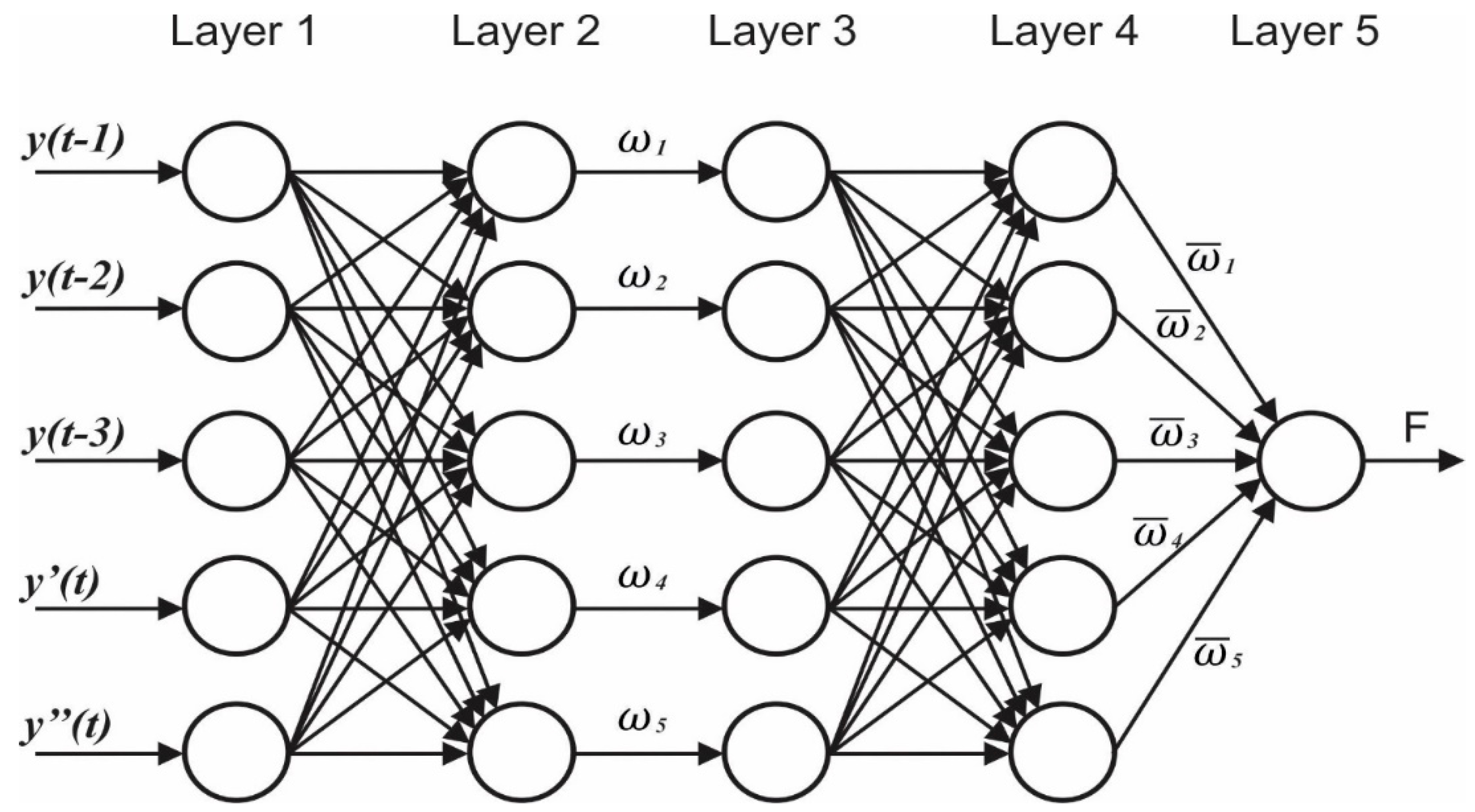
3.2. Machine Learning Approach of Proposed Feedforward ANFIS
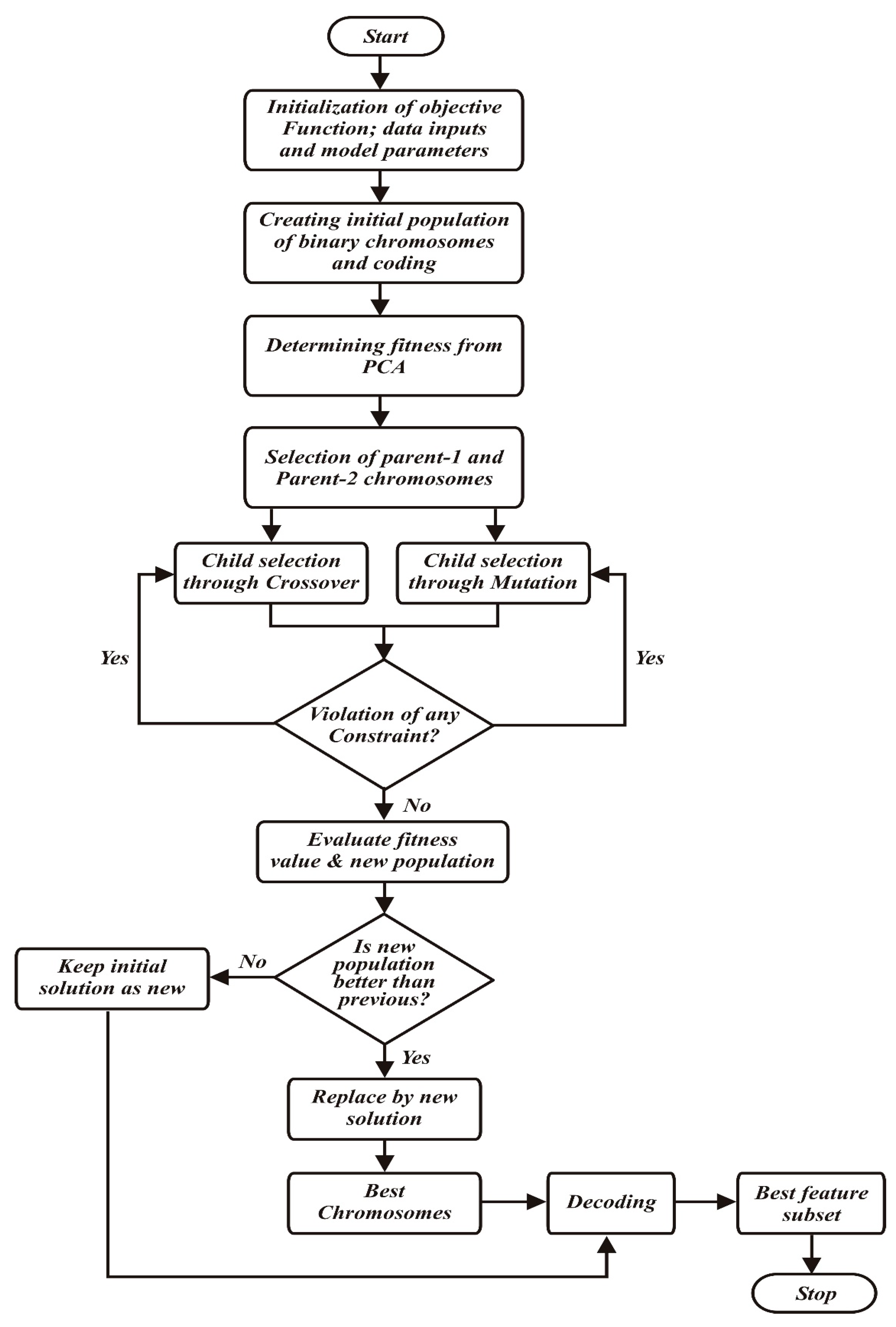
3.3. BGA-PCA for Feature Selection
3.3.1. Initialization of Data Inputs and Model Paraments
3.3.2. Initial Population
3.3.3. Determining Fitness from PCA
3.3.4. Selection or Reproduction
3.3.5. Convergence Condition and Final Feature Subset
- When a maximum number of iterations is reached;
- If fitness values are not better than the previous.
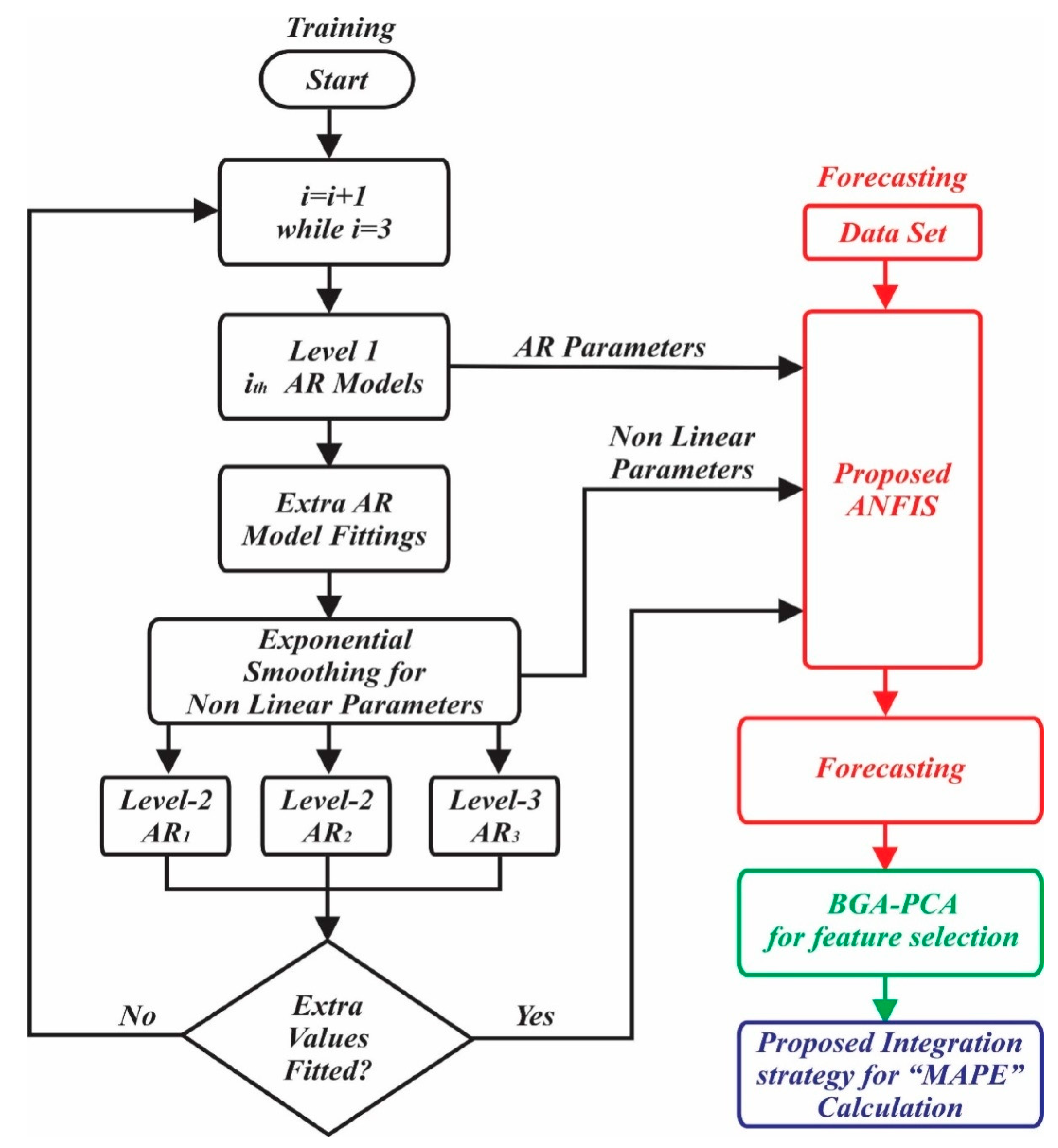
3.4. Proposed Integration Strategy
4. Model Evaluation
5. Results and Discussion
6. Conclusions and Future Studies
Author Contributions
Funding
Institutional Review Board Statement
Informed Consent Statement
Data Availability Statement
Conflicts of Interest
References
- Gellings, C.W. The perspective of the man who coined the term ‘DSM’. Energy Policy 1996, 24, 285–288. [Google Scholar] [CrossRef]
- Asif, R.M.; Ur Rehman, A.; Ur Rehman, S.; Arshad, J.; Hamid, J.; Tariq Sadiq, M.; Tahir, S. Design and analysis of robust fuzzy logic maximum power point tracking based isolated photovoltaic energy system. Eng. Rep. 2020, 2, e12234. [Google Scholar] [CrossRef]
- Bayindir, R.; Colak, I.; Fulli, G.; Demirtas, K. Smart grid technologies and applications. Renew. Sustain. Energy Rev. 2016, 66, 499–516. [Google Scholar] [CrossRef]
- Malik, F.H.; Lehtonen, M. A review: Agents in smart grids. Electr. Power Syst. Res. 2016, 131, 71–79. [Google Scholar] [CrossRef]
- Siddique, M.A.B.; Khan, M.A.; Asad, A.; Rehman, A.U.; Asif, R.M.; Rehman, S.U. Maximum Power Point Tracking with Modified Incremental Conductance Technique in Grid-Connected PV Array. In Proceedings of the 2020 5th International Conference on Innovative Technologies in Intelligent Systems and Industrial Applications (CITISIA), Sydney, Australia, 25–27 November 2020; pp. 1–6. [Google Scholar]
- Fallah, S.N.; Ganjkhani, M.; Shamshirband, S.; Chau, K. Computational Intelligence on Short-Term Load Forecasting: A Methodological Overview. Energies 2019, 12, 393. [Google Scholar] [CrossRef] [Green Version]
- Wang, F.; Xiang, B.; Li, K.; Ge, X.; Lu, H.; Lai, J.; Dehghanian, P. Smart households’ aggregated capacity forecasting for load aggregators under incentive-based demand response programs. IEEE Trans. Ind. Appl. 2020, 56, 1086–1097. [Google Scholar] [CrossRef]
- Khan, F.; Siddiqui, M.A.B.; Rehman, A.U.; Khan, J.; Asad, M.T.S.A.; Asad, A. IoT Based Power Monitoring System for Smart Grid Applications. In Proceedings of the 2020 International Conference on Engineering and Emerging Technologies (ICEET), Lahore, Pakistan, 22–23 February 2020; pp. 1–5. [Google Scholar]
- Du, P.; Lu, N.; Zhong, H. Demand Response in Smart Grids. In Demand Response in Smart Grids; Chapter 1; Springer: Cham, Switzerland, 2019; Volume 1, p. 66. [Google Scholar] [CrossRef]
- Vahid-Ghavidel, M.; Mahmoudi, N.; Mohammadi-Ivatloo, B. Self-scheduling of demand response aggregators in short-term markets based on information gap decision theory. IEEE Trans. Smart Grid 2019, 10, 2115–2126. [Google Scholar] [CrossRef]
- Dash, P.K.; Liew, A.C.; Rahman, S. Fuzzy neural network and fuzzy expert system for load forecasting. IET Proc. Gener. Transm. Distrib. 1996, 143, 106–114. [Google Scholar] [CrossRef]
- Bak, G.; Bae, Y. Predicting the Amount of Electric Power Transaction Using Deep Learning Methods. Energies 2020, 13, 6649. [Google Scholar] [CrossRef]
- Hamza, A.S.H.; Abdel-Gawad, N.M.; Salama, M.M.; Hegazy, A.; El-Debeiky, S. Electric load forecast for developing countries. In Proceedings of the 11th IEEE Mediterranean Electrotechnical Conference (IEEE Cat. No.02CH37379), Cairo, Egypt, 7–9 May 2002; Volume 1, pp. 429–441. [Google Scholar] [CrossRef]
- Nadeem, A.; Arshad, N. PRECON: Pakistan residential electricity consumption dataset. In e-Energy 2019—10th ACM International Conference on Future Energy Systems; Association for Computing Machinery: New York, NY, USA, 2019. [Google Scholar]
- Widén, J.; Lundh, M.; Vassileva, I.; Dahlquist, E.; Ellegård, K.; Wäckelgård, E. Constructing load profiles for household electricity and hot water from time-use data—Modelling approach and validation. Energy Build. 2009, 41, 753–768. [Google Scholar] [CrossRef]
- Bartels, R.; Fiebig, D.G. Metering and modelling residential enduse electricity load curves. J. Forecast. 1996, 15, 415–426. [Google Scholar] [CrossRef]
- Rehman, A.U.; Naqvi, R.A.; Rehman, A.; Paul, A.; Sadiq, M.T.; Hussain, D. A Trustworthy SIoT Aware Mechanism as an Enabler for Citizen Services in Smart Cities. Electronics 2020, 9, 918. [Google Scholar] [CrossRef]
- Alahmed, A.S.; Almuhaini, M.M. Hybrid top-down and bottom-up approach for investigating residential load compositions and load percentages. arXiv 2020, arXiv:2004.12940. [Google Scholar]
- Narayan, N.; Qin, Z.; Popovic-Gerber, J.; Diehl, J.C.; Bauer, P.; Zeman, M. Stochastic load profile construction for the multi-tier framework for household electricity access using off-grid DC appliances. Energy Effic. 2020, 13, 197–215. [Google Scholar] [CrossRef] [Green Version]
- Proedrou, E. A comprehensive review of residential electricity load profile models. IEEE Access 2021, 9, 12114–12133. [Google Scholar] [CrossRef]
- Masood, B.; Guobing, S.; Naqvi, R.A.; Rasheed, M.B.; Hou, J.; Rehman, A.U. Measurements and channel modeling of low and medium voltage NB-PLC networks for smart metering. IET Gener. Transm. Distrib. 2021, 15, 321–338. [Google Scholar] [CrossRef]
- Hossain, M.S.; Madlool, N.A.; Rahim, N.A.; Selvaraj, J.; Pandey, A.K.; Khan, A.F. Role of smart grid in renewable energy: An overview. Renew. Sustain. Energy Rev. 2016, 60, 1168–1184. [Google Scholar] [CrossRef]
- Grosz, B.J.; Altman, R.; Horvitz, E.; Mackworth, A.; Mitchell, T.; Mulligan, D.; Shoham, Y. Artificial Intelligence and Life in 2030: One Hundred Year Study on Artificial Intelligence; Stanford University: Stanford, CA, USA, 2016. [Google Scholar]
- Bansal, R.C.; Pandey, J.C. Load forecasting using artificial intelligence techniques: A literature survey. Int. J. Comput. Appl. Technol. 2005, 22, 109–119. [Google Scholar] [CrossRef]
- Del Real, A.J.; Dorado, F.; Durán, J. Energy demand forecasting using deep learning: Applications for the French grid. Energies 2020, 13, 2242. [Google Scholar] [CrossRef]
- Masood, B.; Khan, M.A.; Baig, S.; Song, G.; Rehman, A.U.; Rehman, S.U.; Asif, R.M.; Rasheed, M.B. Investigation of Deterministic, Statistical and Parametric NB-PLC Channel Modeling Techniques for Advanced Metering Infrastructure. Energies 2020, 13, 3098. [Google Scholar] [CrossRef]
- Niu, D.; Wang, Y.; Wu, D.D. Power load forecasting using support vector machine and ant colony optimization. Expert Syst. Appl. 2010, 37, 2531–2539. [Google Scholar] [CrossRef]
- Saini, L.M. Peak load forecasting using Bayesian regularization, Resilient and adaptive backpropagation learning based artificial neural networks. Electr. Power Syst. Res. 2008, 78, 1302–1310. [Google Scholar] [CrossRef]
- Yoon, B.; Yoon, C.; Park, Y. On the development and application of a self–organizing feature map–based patent map. R&D Manag. 2002, 32, 291–300. [Google Scholar] [CrossRef]
- Brandstetter, P.; Chlebis, P.; Simonik, P. Active power filter with soft switching. Int. Rev. Electr. Eng. 2010, 5, 2516–2526. [Google Scholar]
- Leung, K.F.; Leung, F.H.F.; Lam, H.K.; Ling, S.H. Application of a modified neural fuzzy network and an improved genetic algorithm to speech recognition. Neural Comput. Appl. 2007, 16, 419–431. [Google Scholar] [CrossRef] [Green Version]
- Moradzadeh, A.; Zakeri, S.; Shoaran, M.; Mohammadi-Ivatloo, B. Short-Term Load Forecasting of Microgrid via Hybrid Support Vector Regression and Long Short-Term Memory Algorithms. Sustainability 2020, 12, 7076. [Google Scholar] [CrossRef]
- Dudek, G. Multilayer perceptron for short-term load forecasting: From global to local approach. Neural Comput. Appl. 2020, 32, 3695–3707. [Google Scholar] [CrossRef] [Green Version]
- Khandelwal, I.; Adhikari, R.; Verma, G. Time series forecasting using hybrid arima and ann models based on DWT Decomposition. Procedia Comput. Sci. 2015, 48, 173–179. [Google Scholar] [CrossRef] [Green Version]
- Liu, J.; Li, C. The Short-Term Power Load Forecasting Based on Sperm Whale Algorithm and Wavelet Least Square Support Vector Machine with DWT-IR for Feature Selection. Sustainability 2017, 9, 1188. [Google Scholar] [CrossRef] [Green Version]
- Siddique, M.A.B.; Asad, A.; Rao, M.; Asif, A.U.R.; Sadiq, M.T.; Ulah, I. Implementation of Incremental Conductance MPPT Algorithm with Integral Regulator by using Boost Converter in Grid Connected PV Array. IETE J. Res. 2021, 67. [Google Scholar] [CrossRef]
- Chang, M.-W.; Chen, B. EUNITE Network Competition: Electricity Load Forecasting; National Taiwan University: Taipei, Taiwan, 2001. [Google Scholar]
- Wang, H.; Li, G.; Wang, G.; Peng, J.; Jiang, H.; Liu, Y. Deep learning based ensemble approach for probabilistic wind power forecasting. Appl. Energy 2017, 188, 56–70. [Google Scholar] [CrossRef]
- Ugurlu, U.; Oksuz, I.; Tas, O. Electricity Price Forecasting Using Recurrent Neural Networks. Energies 2018, 11, 1255. [Google Scholar] [CrossRef] [Green Version]
- Zhang, X.; Wang, J.; Zhang, K. Short-term electric load forecasting based on singular spectrum analysis and support vector machine optimized by Cuckoo search algorithm. Electr. Power Syst. Res. 2017, 146, 270–285. [Google Scholar] [CrossRef]
- Abedinia, O.; Amjady, N.; Zareipour, H. A New Feature Selection Technique for Load and Price Forecast of Electrical Power Systems. IEEE Trans. Power Syst. 2017, 32, 62–74. [Google Scholar] [CrossRef]
- Sheikhan, M.; Mohammadi, N. Neural-based electricity load forecasting using hybrid of GA and ACO for feature selection. Neural Comput. Appl. 2012, 21, 1961–1970. [Google Scholar] [CrossRef]
- Urraca, R.; Sanz-Garcia, A.; Fernandez-Ceniceros, J.; Pernia-Espinoza, A.; Martinez-De-Pison, F.J. Improving hotel room demand forecasting with a hybrid GA-SVR methodology based on skewed data transformation, feature selection and parsimony tuning. Log. J. IGPL 2017, 25, 877–889. [Google Scholar] [CrossRef]
- Liu, Y.; Yin, Y.; Gao, J.; Tan, C. Wrapper Feature Selection Optimized SVM Model for Demand Forecasting. In Proceedings of the 2008 The 9th International Conference for Young Computer Scientists, Hunan, China, 18–21 November 2008; pp. 953–958. [Google Scholar]
- Mangai, U.G.; Samanta, S.; Das, S.; Chowdhury, P.R. A Survey of Decision Fusion and Feature Fusion Strategies for Pattern Classification. IETE Tech. Rev. 2010, 27, 293–307. [Google Scholar] [CrossRef]
- Kilimci, Z.H.; Akyuz, A.O.; Uysal, M.; Akyokus, S.; Uysal, M.O.; Atak Bulbul, B.; Ekmis, M.A. An Improved Demand Forecasting Model Using Deep Learning Approach and Proposed Decision Integration Strategy for Supply Chain. Complexity 2019, 2019, 9067367. [Google Scholar] [CrossRef] [Green Version]
- Nguyen, G.; Dlugolinsky, S.; Bobák, M.; Tran, V.; López García, Á.; Heredia, I.; Malík, P.; Hluchý, L. Machine Learning and Deep Learning frameworks and libraries for large-scale data mining: A survey. Artif. Intell. Rev. 2019, 52, 77–124. [Google Scholar] [CrossRef] [Green Version]
- Jadidi, A.; Menezes, R.; De Souza, N.; De Castro Lima, A.C. Short-term electric power demand forecasting using NSGA II-ANFIS Model. Energies 2019, 12, 1891. [Google Scholar] [CrossRef] [Green Version]
- Cai, J.; Luo, J.; Wang, S.; Yang, S. Feature selection in machine learning: A new perspective. Neurocomputing 2018, 300, 70–79. [Google Scholar] [CrossRef]
- Eseye, A.T.; Lehtonen, M. Short-Term Forecasting of Heat Demand of Buildings for Efficient and Optimal Energy Management Based on Integrated Machine Learning Models. IEEE Trans. Ind. Inform. 2020, 16, 7743–7755. [Google Scholar] [CrossRef]
- Hassanat, A.; Almohammadi, K.; Alkafaween, E.; Abunawas, E. Choosing Mutation and Crossover Ratios for Genetic Algorithms—A Review with a New Dynamic Approach. Information 2019, 10, 390. [Google Scholar] [CrossRef] [Green Version]
- Keerthi Vasan, K.; Surendiran, B. Dimensionality reduction using Principal Component Analysis for network intrusion detection. Perspect. Sci. 2016, 8, 510–512. [Google Scholar] [CrossRef] [Green Version]
- Haq, M.R.; Ni, Z. A new hybrid model for short-term electricity load forecasting. IEEE Access 2019, 7, 125413–125423. [Google Scholar] [CrossRef]
- Elahe, M.F.; Jin, M.; Zeng, P. An Adaptive and Parallel Forecasting Strategy for Short-Term Power Load Based on Second Learning of Error Trend. IEEE Access 2020, 8, 201889–201899. [Google Scholar] [CrossRef]


| Symbols | Description |
|---|---|
| Autoregression objective function | |
| Level-11 Autoregression objective function | |
| Previous period load demand | |
| LF demand | |
| Extra autoregression term for a year of 4 season | |
| Feature selection function | |
| Set of premise parameters |
| Models | Formulations | Description of Variable |
|---|---|---|
| Level I Autoregression Model (AR1) | Variation in Weekly load demand: Special holidays or weekend , peak hour, off-peak hour | |
| Level I Autoregression Model (AR2) | AR2 is modeled by adding season autoregression term , where k = 1,…,4. Pakistan has four seasons such as summer, winter, fall, and spring. | |
| Level I Autoregression Model (AR3) | AR3 model has an extra autoregression term for a year and for the seasons of the year , where k = 1,…,4. | |
| Exponential Smoothing Method | This model is used for the purpose where there is no seasonality in the load. Where = smooth constant, = previous period load demand, and = previous period LF demand | |
| Level II Autoregression Model (AR1) | In level-II, the model is applied on the data of the same series in AR1, but the demand values and residential values from customer demand modeled in the Exponential Smoothing Method are added. | |
| Level II Autoregression Model (AR2) | In level-II, the model is applied on the data of the same series in AR2, but the demand values and residential values from customer demand modeled in the Exponential Smoothing Method are added. | |
| Level II Autoregression Model (AR3) | In level-II, the model is applied on the data of the same series in AR3, but the demand values and residential values from customer demand modeled in the Exponential Smoothing Method are added. |
| Sr. No | Model Parameters | Considered Values |
|---|---|---|
| 1. | Population Size | 48 |
| 2. | Selection probability | 1 |
| 3. | Selection Mechanism | Tournament selection |
| 4. | Crossover probability | 0.95 |
| 5. | Mutation Probability | 0.20 |
| 6. | Maximum iteration | 50 |
| 7. | Stopping criteria | 1. When reached max no. of iteration 2. If fitness values are not better than the previous |
| Proposed Algorithm | |
|---|---|
| Step 1: | According to Table 3, adjust the simulation parameters. |
| Step 2: | Compute y(t) and and for different objective functions. |
| Step 3: | Generate random estimation for feedback ANFIS model consists of five stages. |
| Step 4: | Evaluate feature selection with BGA-PCA |
| Step 5: | Compute for the different objective function of |
| Step 6: | Compute for 10 houses |
| Step 7: | Compute |
| Step 8 | Plot of figures for MAPE of four seasons |
| Customer Type. | Without Proposed Integration | With Proposed Integration | With Proposed Integration & BGA-PCA feature selection | With Proposed Integration Improvement Percentage | With Proposed Integration & Machine Learning Improvement Percentage | Over All Improvement Percentage | |||||||||
|---|---|---|---|---|---|---|---|---|---|---|---|---|---|---|---|
| Summer MAPE % | Fall MAPE % | Winter MAPE % | Spring MAPE % | Summer MAPE % | Fall MAPE % | Winter MAPE % | Spring MAPE % | Summer MAPE % | Fall MAPE % | Winter MAPE % | Spring MAPE % | ||||
| House 1 | 2.97 | 3.01 | 3.07 | 2.83 | 2.08 | 2.19 | 2.23 | 2.06 | 1.72 | 1.79 | 1.76 | 1.71 | 39% | 23% | 16% |
| House 2 | 2.88 | 3.02 | 3.06 | 2.67 | 2.10 | 2.19 | 2.20 | 2.02 | 1.69 | 1.67 | 1.84 | 1.67 | 37% | 24% | 13% |
| House 3 | 2.87 | 2.98 | 3.08 | 2.84 | 2.16 | 2.17 | 2.29 | 2.02 | 1.82 | 1.75 | 1.81 | 1.71 | 36% | 22% | 14% |
| House 4 | 2.84 | 2.94 | 3.09 | 2.89 | 2.10 | 2.19 | 2.18 | 2.08 | 1.73 | 1.80 | 1.84 | 1.69 | 38% | 21% | 16% |
| House 5 | 2.91 | 2.96 | 3.09 | 3.01 | 2.20 | 2.14 | 2.16 | 2.07 | 1.72 | 1.72 | 1.77 | 1.75 | 40% | 23% | 17% |
| House 6 | 2.81 | 2.94 | 2.99 | 2.98 | 2.19 | 2.11 | 2.16 | 2.02 | 1.81 | 1.78 | 1.81 | 1.64 | 38% | 20% | 18% |
| House 7 | 2.88 | 3.08 | 2.98 | 2.94 | 2.06 | 2.13 | 2.17 | 2.06 | 1.66 | 1.77 | 1.82 | 1.60 | 41% | 23% | 18% |
| House 8 | 2.9 | 3.04 | 2.97 | 2.85 | 2.01 | 2.12 | 2.15 | 2.06 | 1.67 | 1.85 | 1.76 | 1.65 | 41% | 20% | 21% |
| House 9 | 2.94 | 3.06 | 3.06 | 2.84 | 2.10 | 2.16 | 2.11 | 2.07 | 1.60 | 1.76 | 1.79 | 1.69 | 41% | 23% | 18% |
| House 10 | 2.95 | 2.99 | 3.08 | 2.83 | 2.04 | 2.14 | 2.30 | 2.04 | 1.60 | 1.83 | 1.82 | 1.61 | 39% | 24% | 15% |
| Average | 2.90 | 3.00 | 3.05 | 2.87 | 2.10 | 2.15 | 2.20 | 2.05 | 1.70 | 1.77 | 1.80 | 1.67 | 39% | 22% | 17% |
| Results [53] Novel Hybrid STLF Model Five Regions in Australia | Results [54] Second Learning of Error Trend Model on Different Regions | Results (Proposed Model) 10 Residential Buildings | |||
|---|---|---|---|---|---|
| Season | Min MAPE % | Season | Min MAPE % | Season | Min MAPE % |
| Summer (July–Sep) | 1.68 | Summer | 1.84 | Summer (July–August) | 1.70 |
| Fall (Oct–Dec) | 2.71 | Fall | 1.87 | Fall (Oct–Nov) | 1.77 |
| Winter (Jan–Mar) | 2.28 | Winter | 1.66 | Winter (Jan–Feb) | 1.80 |
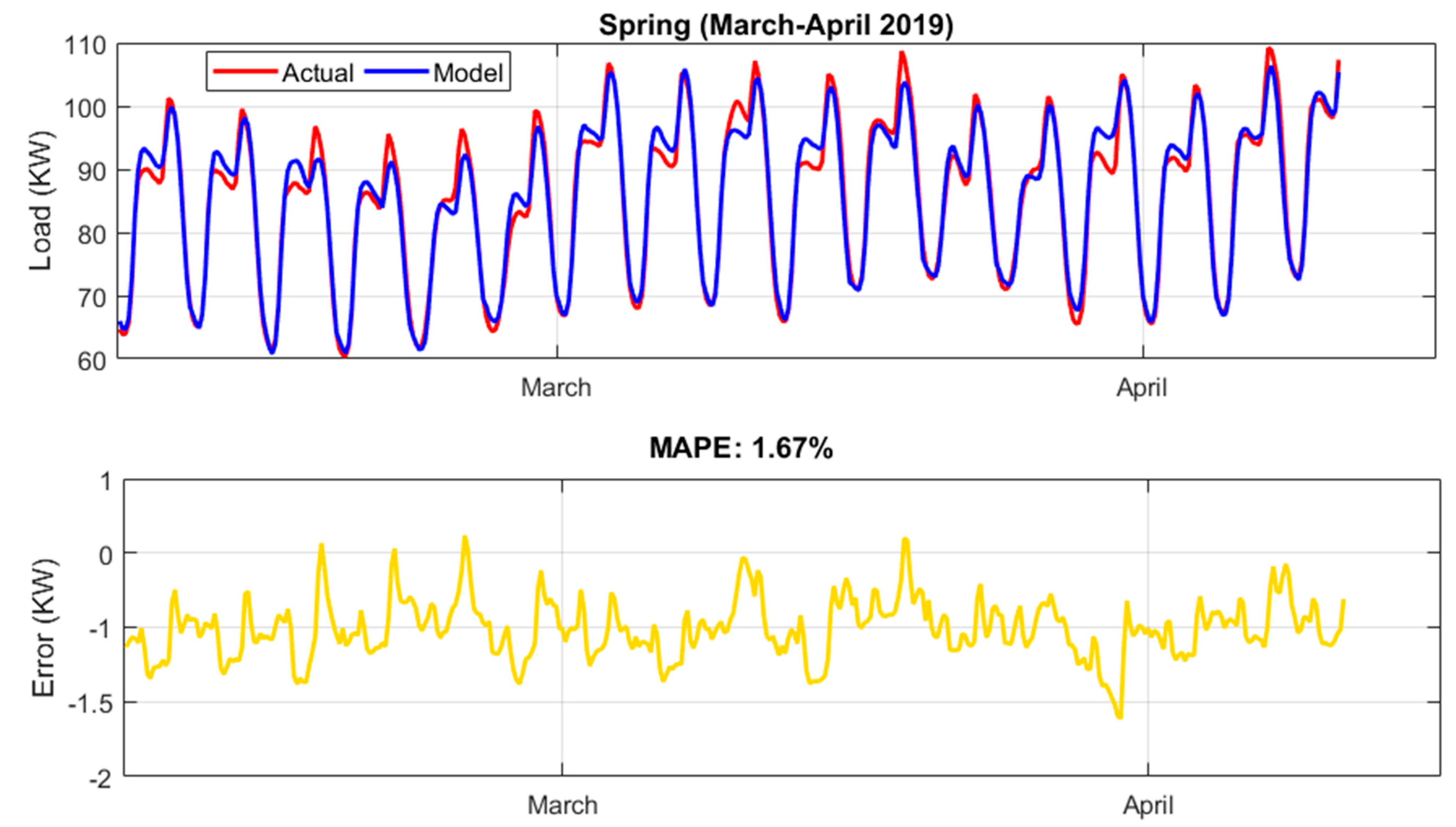
| Spring (April–June) | 2.29 | Spring | 1.80 | Spring | 1.67 |
Publisher’s Note: MDPI stays neutral with regard to jurisdictional claims in published maps and institutional affiliations. |
© 2021 by the authors. Licensee MDPI, Basel, Switzerland. This article is an open access article distributed under the terms and conditions of the Creative Commons Attribution (CC BY) license (https://creativecommons.org/licenses/by/4.0/).
Share and Cite
Yousaf, A.; Asif, R.M.; Shakir, M.; Rehman, A.U.; S. Adrees, M. An Improved Residential Electricity Load Forecasting Using a Machine-Learning-Based Feature Selection Approach and a Proposed Integration Strategy. Sustainability 2021, 13, 6199. https://doi.org/10.3390/su13116199
Yousaf A, Asif RM, Shakir M, Rehman AU, S. Adrees M. An Improved Residential Electricity Load Forecasting Using a Machine-Learning-Based Feature Selection Approach and a Proposed Integration Strategy. Sustainability. 2021; 13(11):6199. https://doi.org/10.3390/su13116199
Chicago/Turabian StyleYousaf, Adnan, Rao Muhammad Asif, Mustafa Shakir, Ateeq Ur Rehman, and Mohmmed S. Adrees. 2021. "An Improved Residential Electricity Load Forecasting Using a Machine-Learning-Based Feature Selection Approach and a Proposed Integration Strategy" Sustainability 13, no. 11: 6199. https://doi.org/10.3390/su13116199