Abstract
Commutation failure at the inverter side of an MIDC (multi-infeed HVDC) is usually caused by AC system faults. Suppose the converter bus voltage cannot recover to the normal operation level in time: in that case, the commutation failure will then develop into more severe subsequent commutation failures or even DC blocking, which will severely threaten the security and stability of the system. Dynamic reactive power compensation equipment (DRPCE) can offer voltage support during accident recovery, stabilize voltage fluctuation and inhibit any subsequent commutation failure risk. This paper proposes the optimal DRPCE configuration scheme for maximizing both inhibitory effect and economic performance. The simulation results on MATLAB-BPA prove the scheme’s correctness and rationality, which can effectively inhibit the risk of subsequent commutation failure and obtain economic benefits.
1. Introduction
1.1. Background and Motivation
In recent years, HVDC technology has played an increasingly significant role in long-distance transmission projects in China [1]. However, the thyristor converter valves used in the HVDC converter station have no self-closing ability. AC system faults lead to the sudden drop of converter bus voltage, which can easily lead to commutation failure [2]. If the converter bus voltage fails to recover to the normal level, it may develop into subsequent commutation failures in an MIDC, resulting in system derating operation or even DC blocking [3]. Especially in an MIDC system, DC-infeed points are relatively close. As a result, converter stations have a very close electrical connection with each other. The fluctuation of electric quantities of a single line can easily affect other lines and cause a regional cascading failure. Therefore, it is necessary to take corresponding measures to inhibit the risk of an MIDC commutation failure. Installing DRPCE to support the AC bus voltage has been proved to be useful [4]. How to choose a reasonable configuration scheme, then, seems to be of prominent practical and applicable significance.
1.2. Reference Survey
At present, there are several ways to inhibit subsequent commutation failure: converter topology transformation, DC system control and reactive power compensation at the grid side. Among these, the method of converter topology transformation can fundamentally solve the problem of commutation failure. VSC-HVDC transmission technology adopts fully-controlled IGBTs, which have a self-closing ability. Consequently, the occurrence of commutation failure can be completely avoided [5]. However, considering the high construction cost, the limitation of transmission capacity and voltage level, VSC-HVDC will not be able to replace the existing LCC-HVDC transmission mode for a long time [6]. At present, DC system controls, such as constant turn-off angle control [7], low voltage current limiting control [8] and other methods, are commonly used to inhibit subsequent commutation failure. However, at the same time as the DC system control method improves the converting margin of the inverters, it inevitably increases reactive power loss, which is not conducive to the recovery of system failures.
DRPCE can quickly react to emit a large amount of reactive power within a short time after the first commutation failure occurs, provide effective voltage support for the commutation bus, suppress voltage fluctuations and inhibit the development of subsequent DC commutation failure. However, current studies on the configuration method of DRPCE are not comprehensive. The results focus mainly on qualitative research, such as the effectiveness of inhibition and installation location selection. Few studies have been done on the further optimization of the DRPCE configuration, such as type and capacity. In [9], the compensation performance of SVC and a synchronous condenser has been compared. The results show that the synchronous condenser performs better than SVC in most situations. Likewise, [10] verifies the effectiveness of installing STATCOMs to inhibit commutation failure and considers the location effect, while [11] uses SVC to improve the fault recovery performance of HVDC systems, testing the effectiveness of inhibiting DC blocks. Finally, [12] proposes a method to select the weak areas for DRPCE installation, but its consideration of subsequent commutation failure is insufficient.
1.3. Proposed Method and Contribution of This Paper
Based on the above research, this paper proposes an optimal configuration scheme for DRPCE to inhibit the risk of subsequent commutation failure in MIDC. The optimal configuration model is established, considering installation location, type and capacity. The improved PSO (Particle Swarm Optimization) algorithm and AHP-TOPSIS (Analytic Hierarchy Process-Technique for Order Preference by Similarity to an Ideal Solution) evaluation method are used to solve the model and select the optimal result from the candidate ones. The proposed dynamic reactive power compensation scheme is then tested for practicality and effectiveness against subsequent commutation failure inhabitation using the example of MIDC in the East China Power Grid.
This paper is organized as follows: In Section 2, the mechanism of commutation failure is detailed and analyzed, and the process of development from the first commutation failure to subsequent commutation failures is further introduced. Section 3 explains the mechanism of DRPCE for inhibiting subsequent commutation failures and proposes an index to evaluate the inhibitory effect. Then the optimal configuration steps are shown in Section 4. The configuration model of dynamic reactive power compensation is considered from the aspects of installation location, type and capacity, respectively. Section 5 provides an optimal configuration model with the solving algorithm as well as the specific process. Correctness and practicability are then tested and verified in Section 6. Finally, Section 7 draws conclusions.
2. Mechanism Analysis of MIDC Subsequent Commutation Failure
2.1. Mechanism of Commutation Failure
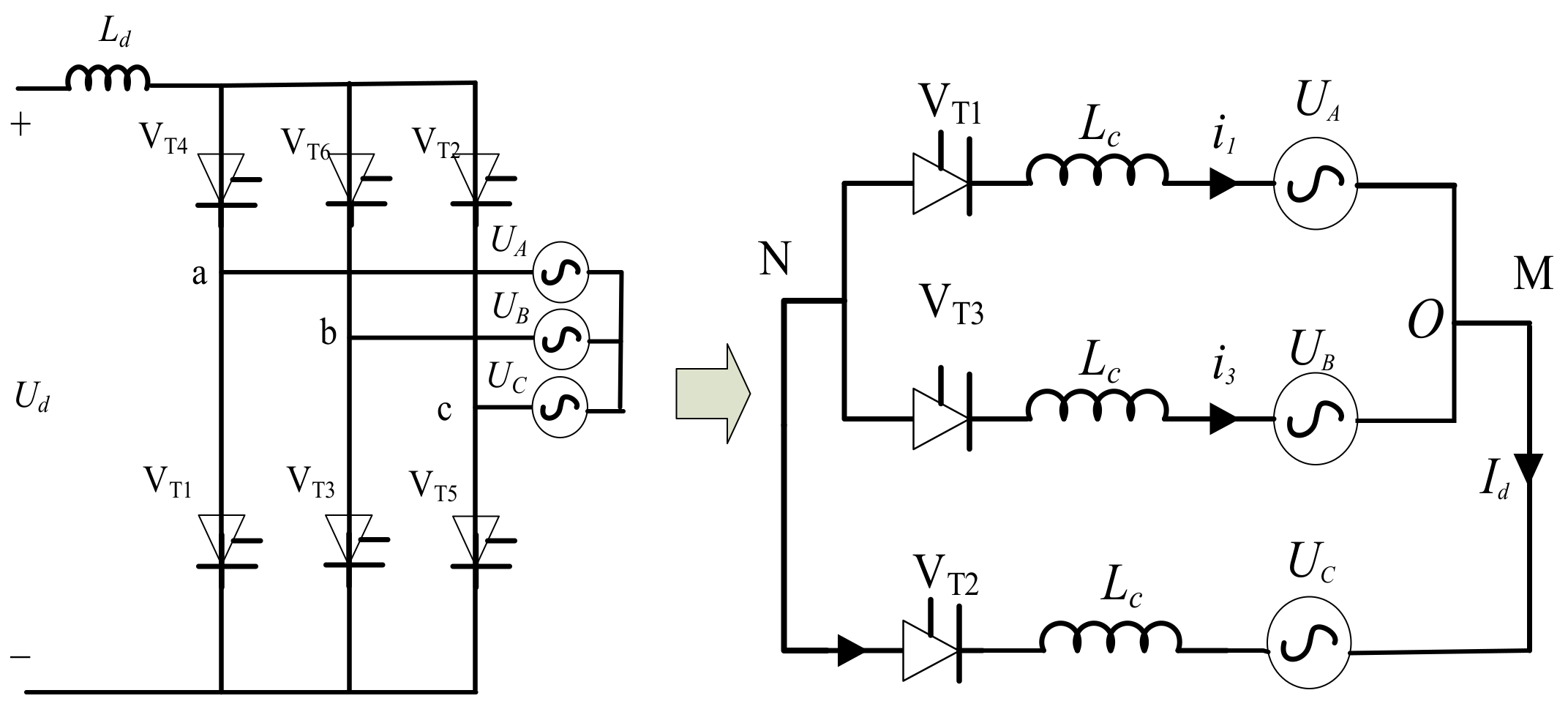
A traditional HVDC transmission project mainly uses a three-phase bridge converter, and commutation failure is one of its most common faults. In the commutation process between the two bridge arms of the converter, the valve which is ready to be shut off fails to be blocked in time or the commutation cannot be completed smoothly, which will both cause the valve to re-conduct. This situation is called commutation failure. Figure 1 and Figure 2 show the commutation process of the simplified inverter valve VT1 to VT3.
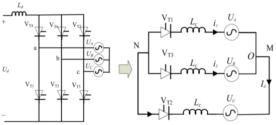
Figure 1.
DC commutation process.
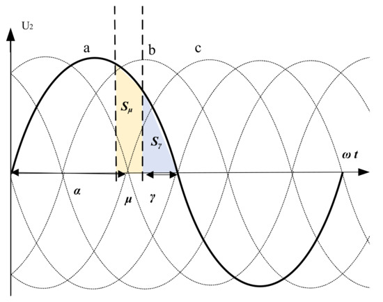
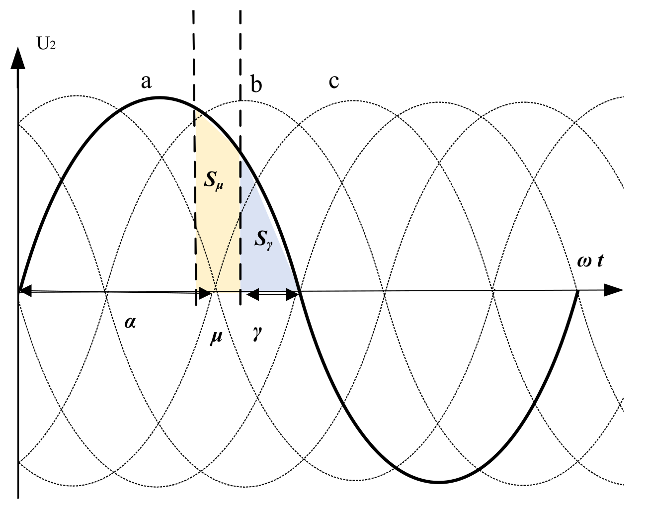
Figure 2.
The waveform of commutation voltage.
In the process of DC commutation, the phase change process starts after a trigger delay angle α, μ is the overlap angle corresponding to the current transfer process in the phase change process and γ is the turn-off angle corresponding to the blocking capacity of the valve after the phase change. During the conduction state transition from VT2, VT1 to VT2, UA > UB, the current flowing through VT3 increases slowly:
where UL is the converter bus voltage and I3 and I1 are the currents flowing through VT3 and VT1, respectively.
In the commutation process, the direct current Id can be regarded as constant, then Equation (1) is integrated with time t. We can get the following results:
Sμ is the voltage–time area required to complete a commutation, as shown in Figure 2. The sum of commutation voltage–time area and turn-off voltage–time area S(μ + γ) can be expressed as:
Subsequently, the turn-off voltage–time area can be expressed as:
It can be seen from Equation (4) that the turn-off voltage–time area is affected by the trigger delay angle α, direct current Id, AC commutation voltage UL and commutation inductance LC. In practical engineering, the causes of commutation failure usually include trigger pulse loss, converter valve short circuit and inverter side AC faults, most of which are caused by AC system faults. The sudden drop in commutation voltage and the sudden increase in direct current caused by an AC system fault will reduce the turn-off angle. The turn-off voltage–time area is then insufficient, which leads to commutation failure [12].
2.2. First Commutation Failure and Subsequent Commutation Failure
According to the occurrence order and characteristics, commutation failure can be divided into first commutation failure and subsequent commutation failure [13]. Because the time between AC system failure and the first commutation failure is very short, the first commutation failure is often difficult to avoid [14]. Subsequent commutation failure refers to the continuous commutation failure of a single DC or the successive commutation failure of adjacent DCs because the converter bus voltage does not recover in time after the first commutation failure. Especially in an MIDC system, there are close electrical connections between inverter stations. Suppose no intervention measures are taken after the first commutation failure: in that case, it easily develops into a large-scale DC cascading fault [15] or even DC blocking, which will cause destructive consequences to the stable operation of the system.
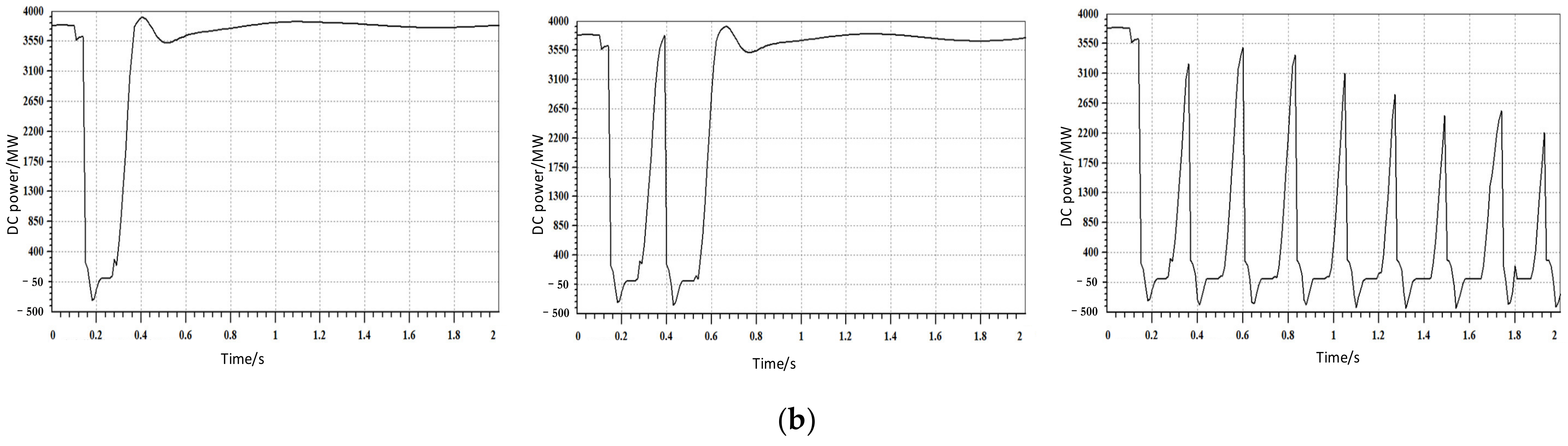
Take the operation status of East China Power Grid in the summer of 2018 as an example (Figure 3). To reveal the process of commutation failure and how the first commutation failure develops into subsequent commutation failure, a three-phase short circuit fault is set at the midpoint of a 500 kV Line near the SX converter station at 0.1 s, and the fault is removed after 5, 10 and 20 cycles respectively. The power observation of YS HVDC and nearby YH HVDC is shown in Figure 4.
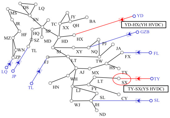
Figure 3.
East China Power Grid in the summer of 2018.
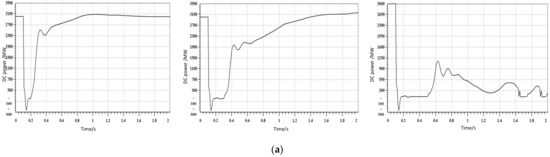
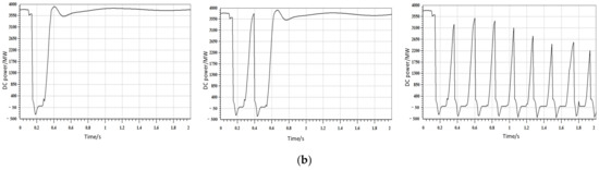
Figure 4.
Power observation of YS/YH HVDC under 5, 10 and 20 cycles of fault. (a) Power observation of YS HVDC under 5, 10 and 20 cycles of fault. (b) Power observation of YH HVDC under 5, 10 and 20 cycles of fault.
It can be seen from the figure that the AC system fault at 0.1 s almost instantaneously caused the first commutation failure of YS HVDC and a short-term interruption of DC transmission power. The nearby YH HVDC is also affected and the first commutation failure occurs, lagging slightly behind YS HVDC. If the fault only lasts for 5 cycles, the two HVDC systems can both recover automatically after short-time adjustment. If the fault is removed after 10 cycles, it can be seen from the waveform that the recovery time of YS HVDC is prolonged, which leads to the second commutation failure of YH HVDC. If the fault is removed after 20 cycles, YS HVDC can no longer return to normal operation, and the DC power will be interrupted again. The adjacent YH HVDC will also fail in continuous commutation due to the power oscillation of YS HVDC.
The commutation failure of YH HVDC and the two commutation failures of YS HVDC at 1.64 s and 1.92 s under the condition of 20 cycles of fault observed in the figure are all subsequent commutation failures caused by the first commutation failure of YS HVDC. After the first commutation failure occurrence, the DC power recovery process will absorb a lot of reactive power from the system and worsen the voltage. Insufficient subsequent turn-off voltage–time area will then lead to subsequent commutation failure of this DC and adjacent DCs, threatening the operation safety of the system. Therefore, measures must be taken to inhibit the risk of subsequent commutation failure caused by the first commutation failure.
3. Effect Analysis of DRPCE for Inhibiting Subsequent Commutation Failure of MIDC
3.1. Mechanism of DRPCE for Inhibiting Subsequent Commutation Failure
In the DC system, the main cause of commutation failure of the inverter side is the insufficiency of turn-off voltage–time area (γ < γmin) [16]. The turn-off angle can be expressed as Equation (5).
The partial derivatives of the variables on the right side of Equation (5) are as follows:
where γ, β, UL and XL refer to the turn-off angle, the advance trigger angle, the effective bus voltage value and the commutation reactance of the inverter, respectively; Id is the direct current and n is the transformer transformation ratio of the inverter station.
It can be seen from Equations (5) and (6) that γ is directly proportional to UL and β, while inversely proportional to Id and XL. DRPCE can quickly offer reactive power compensation in case of fault, keep the DC power, sustain the commutation bus voltage UL and increase the turn-off angle γ. As a result, the risk of subsequent commutation failure can be inhibited by configuring the DRPCE.
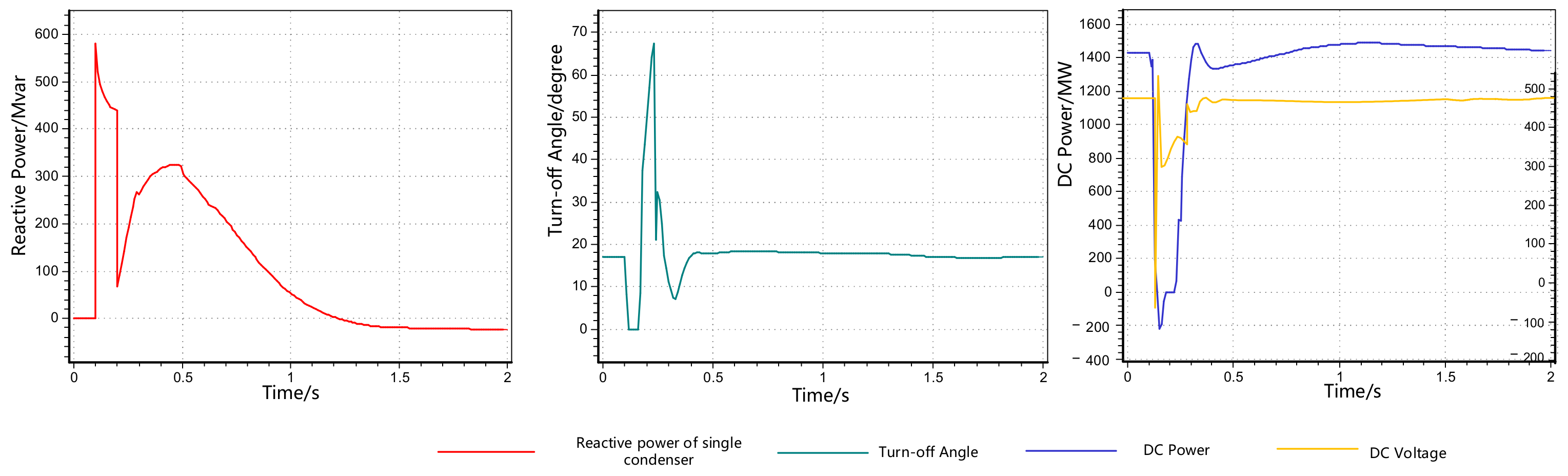
If a fault simulation of a three-phase short circuit is set at the midpoint of a 500 kV line of YH HVDC at 0.1 s, the fault is cleared at 0.5 s. The changes in electric quantity before and after the installation of DRPCE are shown in Figure 5 and Figure 6, respectively.
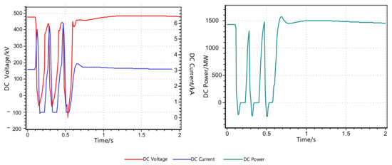
Figure 5.
Diagram of electrical quantity change in case of commutation failure of YH HVDC.
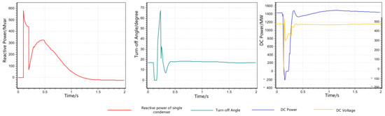
Figure 6.
The effect after installing DRPCE.
From the results shown in Figure 4, it can be seen that the three-phase short circuit fault at 0.1 s caused the commutation failure of YH HVDC: the line voltage dropped, the current rose and the transmission power was interrupted for a short time. As the fault was not cleared in time, the subsequent commutation failures of YH HVDC occurred on the basis of the first commutation failure. The voltage, current and DC power oscillated violently. Figure 5 shows that DRPCE can rapidly generate a large amount of reactive power, provide support for the converter bus, increase the turn-off angle, effectively inhibit the occurrence of subsequent commutation failures and maintain the stable operation of the system.
3.2. Effect Evaluation Index of DRPCE for Inhibiting Subsequent Commutation Failure
Here, the effect evaluation index RMCCF is defined to characterize the inhibitory effect of DRPCE on subsequent commutation failure in MIDC. RMCCF is the product of the shortened probability duration of subsequent commutation failure by installing DRPCE and the DC power weight after the fault occurs. The larger the RMCCF is, the better the inhibitory effect of commutation failure is. Furthermore, the operation mode of the system affects the possibility of commutation failure as well. Consider the system has N typical operation modes and RMCCF can be expressed as Equation (7):
where n and N refer to the operation mode and the total number of typical operation modes, respectively; fmode, n is the probability of n; j and z refer to the fault and the total number of faults, respectively; fj is the probability of j; tji − 0 and tji are the duration of commutation failure of DC i before and after reactive power compensation in case of fault j, respectively; Pi is the transmission power of DC i; δi is the power weight coefficient which is calculated by the power transmission of each DC in the MIDC system. The larger δi is, the more serious the influence will be when the DC commutation fails.
4. Optimal Configuration Steps of DRPCE
4.1. Installation Location Configuration of DRPCE
According to the principle of local reactive power compensation, the compensation facilities are usually installed nearby. However, in MIDC, there is a strong electrical connection between DC and DC. The interaction between the installation site and the converter station of each subsystem should be considered comprehensively.
The CIGRE working group proposed the concept of multi-infeed interaction factor (MIIF) in 2008 [17]. This revealed that the converter bus voltage can describe the interaction between converter stations of MIDC subsystems. The converter bus m is connected with the three-phase symmetrical reactor. When the voltage of the converter bus decreases by 1%, MIIF refers to the change rate of voltage corresponding to the voltage at the other converter bus j.
Inspired by the definition of MIIF, the voltage coupling factor MIADF (multi-infeed AC/DC factor) can be defined as Equation (11). It characterizes the interaction between AC bus and multi-inverter converter bus in the MIDC system.
where δd is the power weight coefficient of converter bus d; Pd is the power of the converter bus d and Zld and Zll are the mutual-impedance and the self-impedance of AC bus l, respectively.
The higher the MIADF value is, the greater the bus-to-bus interaction is. Stronger interaction means that the compensation at these buses can respond better than those with poor interaction [18]. Therefore, the candidate area for DRPCE installation can be selected by sequencing the MIADF value in the receiving-side grid.
It is then necessary to make the installation nodes from the candidate installation area accurate. If the installed capacity of DRPCE is set as a fixed value △q, and the index Ri is defined, the response level can be evaluated as:
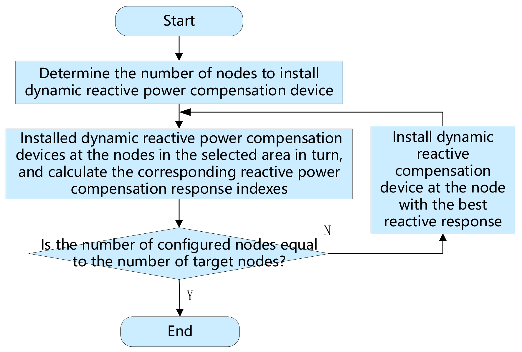
RMCCF (△q) refers to the inhibitory effect of subsequent commutation failure under the configuration of DRPCE of capacity △q, which can be obtained by Equation (7). The higher the value Ri takes at node i, the more sensitive the reactive compensation performed here is. All nodes in the candidate area are sorted according to the index value. The sorting process is carried out by the cycle selection method shown in Figure 7.

Figure 7.
Flow chart of location cycle selection for DRPCE.
4.2. Type and Capacity Configuration of DRPCE
SVC, synchronous condenser and STATCOM are the most commonly used DRPCEs. Among them, the synchronous condenser is a kind of synchronous motor that can generate a large amount of reactive power at the moment of fault, which provides short-circuit capacity and reactive power support for the system, but the response speed is slow and the loss is large. SVC is a kind of typical power electronic-reactive power compensation device, which uses a thyristor as a solid-state switch to control the capacity of the capacitor and reactor in the access system, so as to change the system admittance and control the reactive output power. The advantages of SVC are its fast response speed and continuous reactive power regulation. However, the reactive power compensation capacity of SVC is greatly affected by the system bus voltage. In case of serious fault, the reactive output current will decrease proportionally with the system voltage. The reactive power support capacity is limited. STATCOM is a new type of dynamic reactive power compensation equipment, which has faster response speed and reactive power support capability than SVC. It is insensitive to the external system operating conditions and structural changes. Moreover, it has a wider operation range and larger compensation capacity. Three kinds of common DRPCE have their advantages and disadvantages. In order to achieve comprehensive optimization, the most suitable type of dynamic reactive power compensation equipment should be selected according to the actual economic conditions while meeting the optimization objectives.
In this paper, the DRPCE is considered so as to maximize both the inhibitory effect and optimize economic performance. It is a typical multi-objective optimization problem.
Objective functions
The multi-objective optimization function F has two sub-objective functions, f1 and f2. Among them, f1 is the configuration cost function, and f2 uses the negative value of RMCCF to characterize the inhibitory effect of commutation failure; x is a control variable, representing the type of DRPCE and installation capacity; s is a 0–1 state variable; ci - x is the installation cost of the DRPCE, and the unit price of the DRPCE is pi - x. Qi - x is the reactive power compensation capacity.
Constraints
where: , and represent the conductance, admittance and phase difference between the branches i-j, respectively. , , , , , , and are the lower and upper limits of active power, reactive power, voltage and reactive compensation capacity, respectively.
5. Solving Algorithm and Process
5.1. PSO Algorithm for Adaptive Adjustment of Inertial Weights
PSO (Particle Swarm Optimization) is an intelligent algorithm that uses bird foraging behavior as a reference to simulate the state of a bird population when it is randomly searching for food and find optimal strategies in the search space to solve optimization problems. The direction of the particle update is determined by the location and velocity variables, while the fitness value of the optimized function determines the particle position. Particles always follow the current optimal particle in the whole search space and approach the optimal solution [19] step by step. However, the PSO algorithm may be trapped in a local convergence optimization when searching globally. Considering this disadvantage of PSO, this paper proposes the adaptive adjustment of inertial weights to avoid premature local convergence of the algorithm. The relevant parameter settings are shown in Appendix A.
The speed and position of the first particle in the population in the tth iteration can be expressed as
where and are particle velocity and position, respectively; is the inertial weight; and are learning factors; and are random numbers in range [0,1] and and are individual extremes and population extremes, respectively.
The inertial weight of the particle swarm affects the optimization ability of the algorithm. The larger the inertial weight, the stronger the global search ability of the algorithm. In the iteration, the inertia weight of the algorithm can be adjusted automatically to fit the search process. This can prevent the algorithm falling into a local optimum as early as possible. The formula for adaptive adjustment is as follows:
where: is the inertial weight for the tth iteration and and are the initial and final values of inertial weight, respectively.
5.2. AHP-TOPSIS Evaluation Method
A set of non-inferior solutions on the Pareto frontier can be obtained by optimizing the multi-objective function by PSO. In order to select the most appropriate DRPCE configuration scheme from the obtained non-inferior solutions, this paper uses the improved AHP-TOPSIS evaluation method [20] to objectively evaluate and rank the optimization results, eliminates the subjective influence of each factor, and makes the results more reasonable.
The Euclidean distance between the alternative scheme and the positive ideal/negative ideal scheme can be calculated according to [20]. The closer the distance between the alternative scheme and the positive ideal scheme is, the better the alternative scheme is. Here we define Pi as the relative closeness of each alternative to the positive ideal solution. Si+ is the Euclidean distance between the evaluation index i and the positive ideal index. Similarly, Si- is the Euclidean distance between the evaluation index i and the negative ideal index. One can calculate the Pi of each alternative to the positive ideal scheme as follows:
According to the relative closeness value of the proposed alternative, the scoring criteria are established for the alternative, as shown in Table 1:

Table 1.
Scoring criteria for alternative schemes.
5.3. Solution Steps
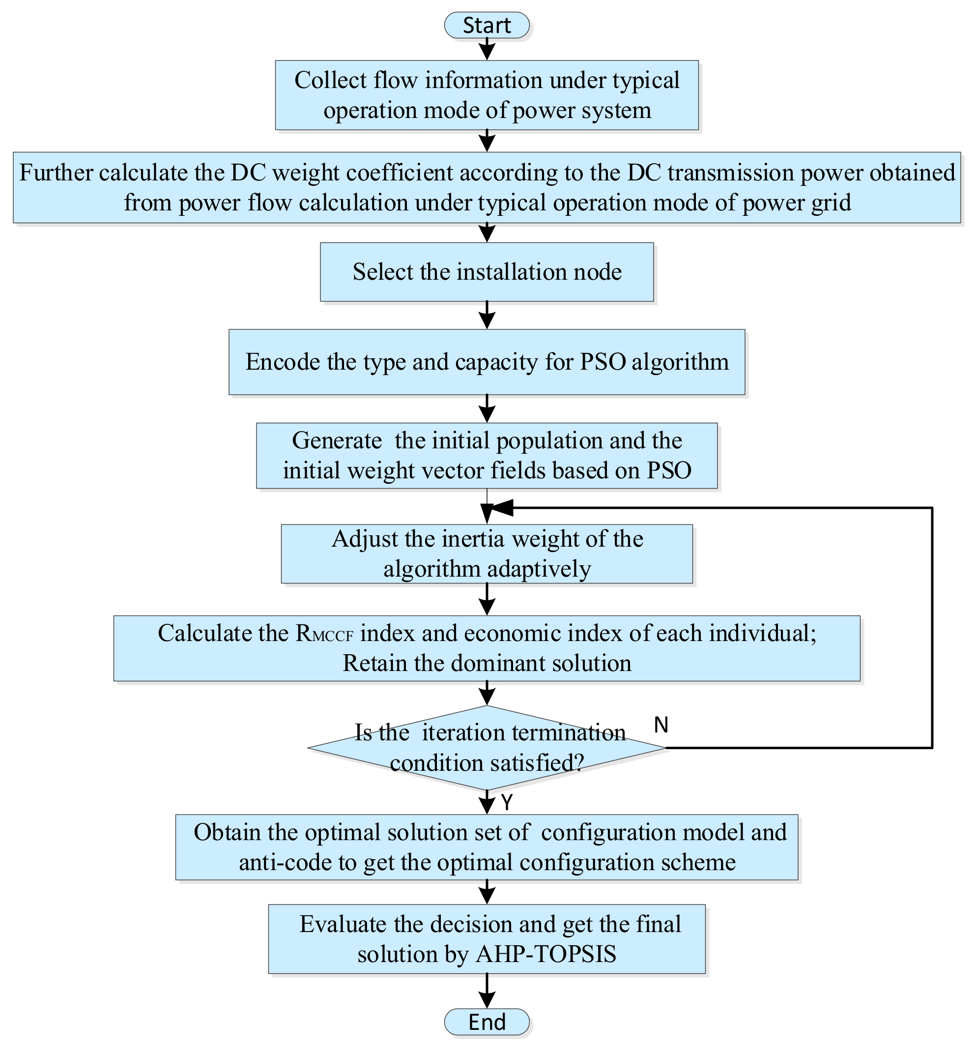
The basic idea of solving the DRPCE configuration problem is to use the improved PSO algorithm for multi-objective optimization and obtain a group of non-inferior solutions on the Pareto front. Subsequently, the AHP-TOPSIS (Analytic Hierarchy Process-Technique for Order Preference by Similarity to an Ideal Solution) evaluation method is used for the group of non-inferior solutions. The most reasonable configuration scheme is selected, and the solution process is shown in Figure 8.
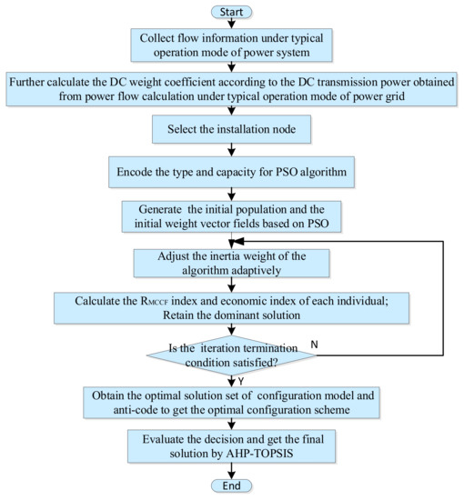
Figure 8.
Flow chart of optimal configuration of DRPCE.
6. Example Analysis
Here we chose the East China Power Grid as an example to analyze and validate the DRPCE optimal configuration scheme for inhibiting subsequent HVDC commutation failures on the simulation platform MATLAB-BPA. The example considers eight DC feeds, as shown in Appendix B. This paper only considers the reactive power compensation at major sites (≥ 500 kV). The DRPCEs used here are SVCs and synchronous condensers. Each device considers four candidate compensation nodes. The installation costs of SVCs and synchronous condensers are set to 38,675 USD and 46,410 USD, respectively. The reactive power compensation unit prices are 46,410 USD/Mvar and 77,350 USD/Mvar respectively [21,22].
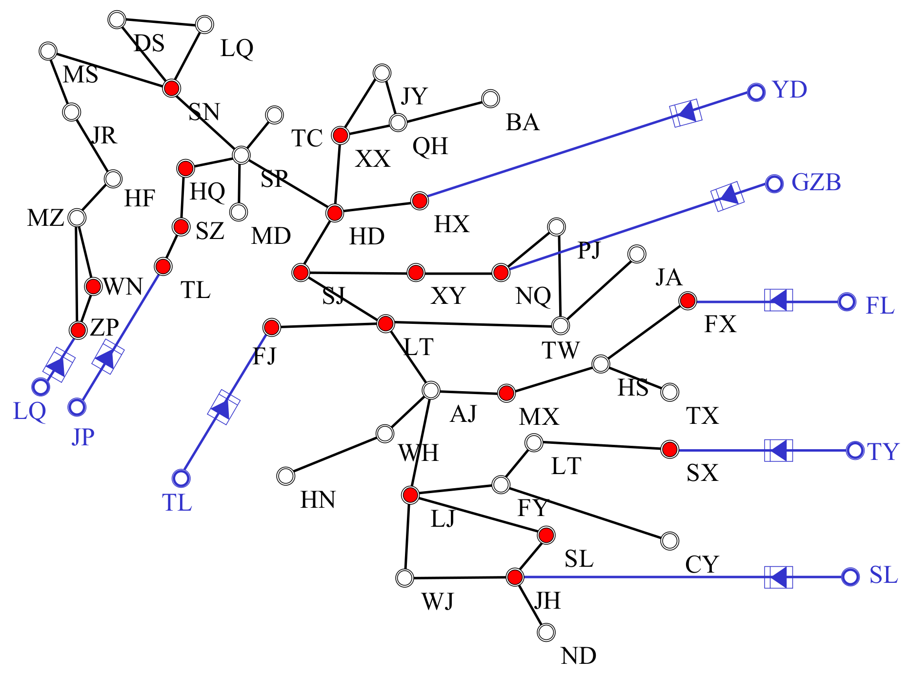
The MIADF values of all nodes are calculated and sorted, and the top 20 nodes (marked in red) are selected as candidate installation areas, as shown in Figure 9.

Figure 9.
Candidate area of DRPCE.
DRPCE is installed at the red nodes in the area, and the nodes are selected and sorted according to the compensation response evaluation index Ri of each node. The results are shown in Table 2.
Table 2.
Installation node of DRPCE.
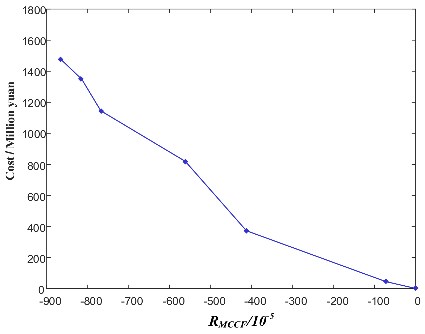
Subsequently, the improved PSO algorithm is used to optimize the type and capacity of dynamic reactive power compensation equipment. Combined with this engineering practice, the capacity of SVC is continuously adjustable, and the single capacity of the synchronous condenser is fixed at 300 Mvar. Through the improved PSO, a group of optimal configuration non-inferior solutions on the Pareto front are obtained, which consider both the economic performance and the inhibitory effect of subsequent commutation failure, as shown in Figure 10.
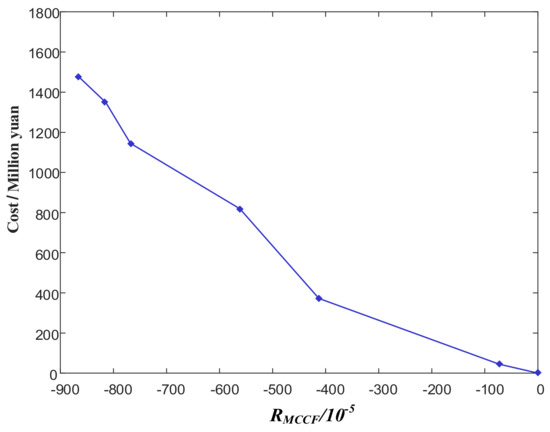
Figure 10.
Dynamic reactive power compensation scheme.
It can be seen from the figure that the inhibitory effect of DRPCE on subsequent commutation failure is positively related to the capacity configuration cost, which indicates that increasing the configuration capacity of DRPCE can effectively improve the inhibitory effect. However, the disadvantage is that it will greatly increase the cost. By observing the changing trend of the curve, it can be seen that the inhibitory effect of DC commutation failure and the increase in cost do not have a simple linear relationship, but a saturation. When the capacity is allocated to a certain extent, the improvement of the inhibitory effect on the subsequent commutation failure of DC is not obvious. At this time, increasing the allocated capacity will only bring a serious economic burden. Therefore, it is necessary to comprehensively evaluate the economic indicators and commutation failure inhibitory effect to select the most reasonable configuration scheme. The configuration scheme and evaluation are shown in Table 3 and Table 4, respectively.
Table 3.
Compensation scheme of DRPCE.
Table 4.
Evaluation on configuration scheme of DRPCE.
According to the analysis in Table 3 and Table 4, the configuration capacity of the synchronous condenser is always higher than that of SVC in the configuration scheme optimized by PSO, proving the conclusion that the reactive power compensation effect of the synchronous condenser is better than that of SVC. However, if we want to pursue economic benefits, we should prioritize the installation of SVC.
As shown in Table 4, the configuration cost of scheme six, which only installed SVC of 175 Mvar in the SJ node and does not install synchronous condensers, is the lowest. Although this configuration scheme achieves the optimal economic performance, the inhibitory effect on subsequent commutation failure is poor. Therefore, it is necessary to comprehensively consider the economic performance and the inhibitory effect of DC commutation failure. The results of AHP-TOPSIS are listed in Table 4. Schemes one, two, three and four achieve good evaluation results. Scheme 3, with the highest score, is selected as the final configuration scheme. The configuration condition of Scheme 3 is shown in Figure 11.
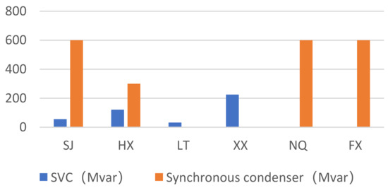
Figure 11.
Optimal configuration scheme of DRPCE.
From the installation position, capacity and type of DRPCE, it can be seen that synchronous condensers with a large capacity are always installed in the DC infeed converter stations. Synchronous condensers installed in converter stations can quickly provide a lot of reactive power support in case of faults, maintain the voltage level of the converter bus and inhibit the risk of subsequent converter failure of an MIDC. SVC installed in some non-converter stations can reduce the indirect impact of a voltage drop in the non-converter buses on MIDC commutation failure. It not only ensures the inhibitory effect of subsequent commutation failure, but also takes the economic performance of the whole scheme into account.
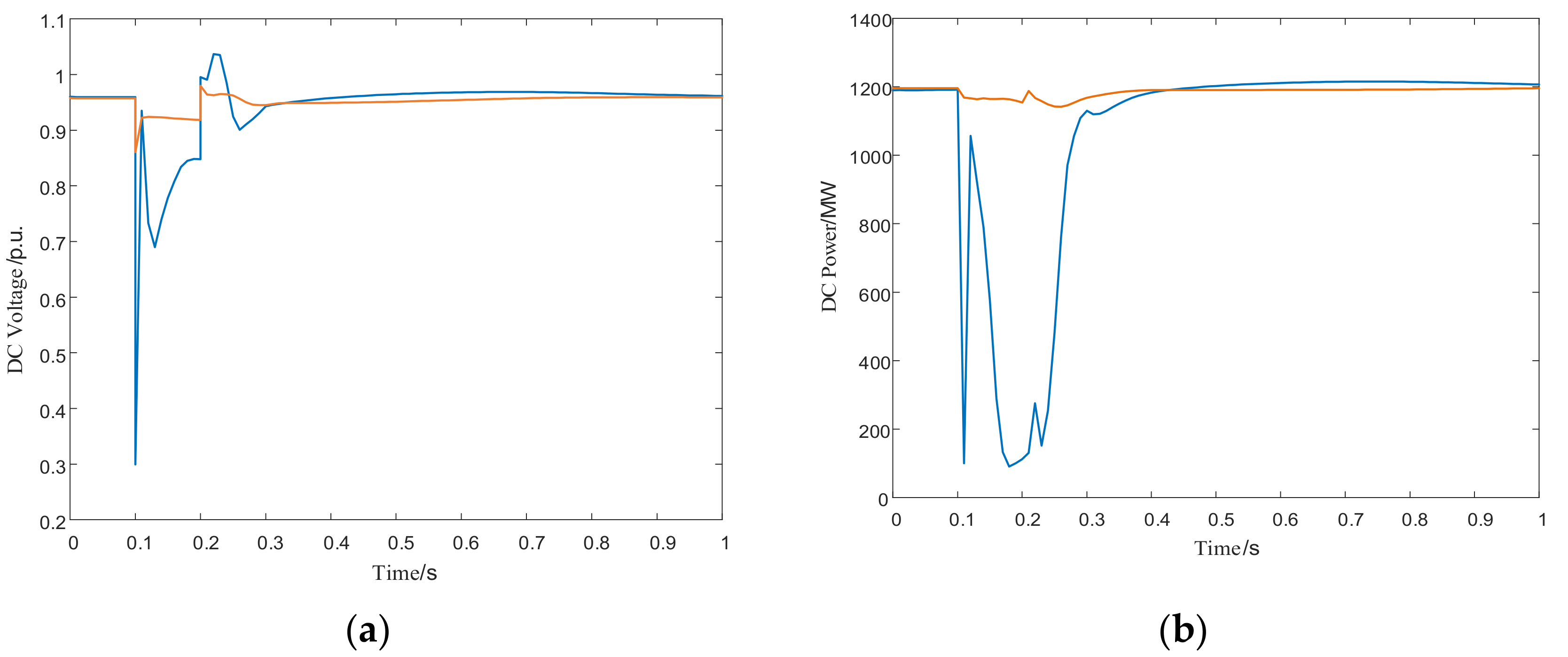
Taking NQ station as an example, a three-phase short circuit fault at the midpoint of a 500 kV line is set at 0.1 s, and the fault is removed after 0.1 s. PSD-BPA is used to observe the voltage and DC power changes before and after the dynamic reactive power compensation equipment is installed in NQ station. The results are shown in Figure 12.
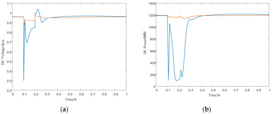
Figure 12.
Change of electrical quantity before and after DRPCE configuration: (a) Change of voltage; (b) Change of DC power.
From the curve comparison in the figures, it can be seen that without DRPCE, the sudden drop of voltage and DC power causes the failure of DC commutation in the NQ converter station. After the first commutation failure, the fault remains for 0.1 s, resulting in the subsequent commutation failures of the converter station, the voltage and DC power secondary drop and then oscillation, seriously threatening the system security. After the DRPCE is configured, it can support the voltage and power drop caused by the fault, stabilize the voltage fluctuation, maintain stable transmission power and effectively inhibit the risk of subsequent commutation failure.
To further verify the rationality of the proposed method, an N-1 scan of 500 kV and above lines under three-phase short circuit fault is carried out, and the average number of commutation failures is counted. The smaller the average number of commutation failures, the stronger the ability to resist the failure—that is to say, the better the inhibitory effect of subsequent commutation failure of DC after the configuration of DRPCE. The statistical results are shown in Table 5.
Table 5.
Configuration effect of DRPCE.
It can be seen from Table 5 that the installation of DRPCE can significantly improve the ability of the system to inhibit the subsequent commutation failure of DC. Compared with the scheme proposed in [12], the joint configuration of SVC and synchronous condenser has a better effect. The average times of commutation failure are less, which verifies the rationality and effectiveness of the proposed method.
7. Conclusions
Based on the mechanism of subsequent commutation failure, this paper proposes a DRPCE configuration scheme to maximize both the economic performance and the risk-inhibitory effect of subsequent commutation failure in an MIDC. The conclusions are as follows:
- (1)
- The mechanism analysis reveals that the main cause of subsequent commutation failure is the insufficient turn-off voltage–time area after the first commutation failure cannot complete subsequent commutations normally. Configuring DRPCE can inhibit the risk of the subsequent commutation failure of an MIDC. Based on this, a corresponding DRPCE configuration model is established, and the installation location, type and capacity are reasonably configured.
- (2)
- Taking economic performance and the inhibitory effect as optimization objectives, an improved PSO algorithm is used to optimize the proposed model for obtaining configuration schemes that meet the optimization objectives. The AHP-TOPSIS evaluation method is used to evaluate and select the optimal one with the highest score as the final scheme (Scheme 3, with the highest score, is selected as the final configuration scheme). The correctness and validity of the method proposed in this paper are verified using the example of the East China Power Network.
Author Contributions
The authors confirm their contributions as follows: Y.Z. proposed the innovations and wrote the paper; F.T. and F.Q. reviewed the simulation results; Y.L. revised the manuscript; X.G. and N.D. approved the final version. All authors have read and agreed to the published version of the manuscript.
Funding
This research was supported by State Key Laboratory of HVDC.
Institutional Review Board Statement
Not applicable.
Informed Consent Statement
Not applicable.
Conflicts of Interest
The authors declare no conflict of interest.
Appendix A
Table A1.
Parameter settings of the PSO algorithm.
Table A1.
Parameter settings of the PSO algorithm.
| Population Size N | Number of Iterations T | Learning Factor c1, c2 | ||
|---|---|---|---|---|
| 60 | 1000 | 1.7 | 0.9 | 0.4 |
Appendix B
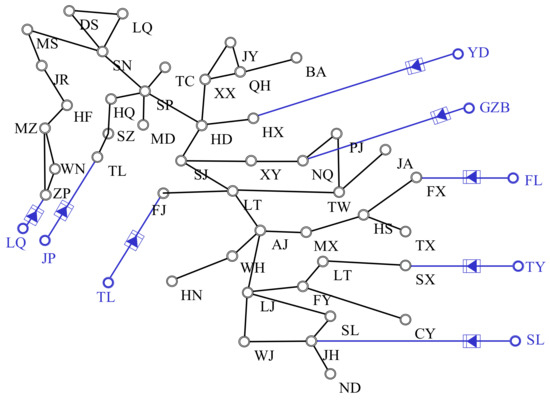
Figure A1.
Diagram of the DC infeed in East China Power Grid.
Figure A1.
Diagram of the DC infeed in East China Power Grid.
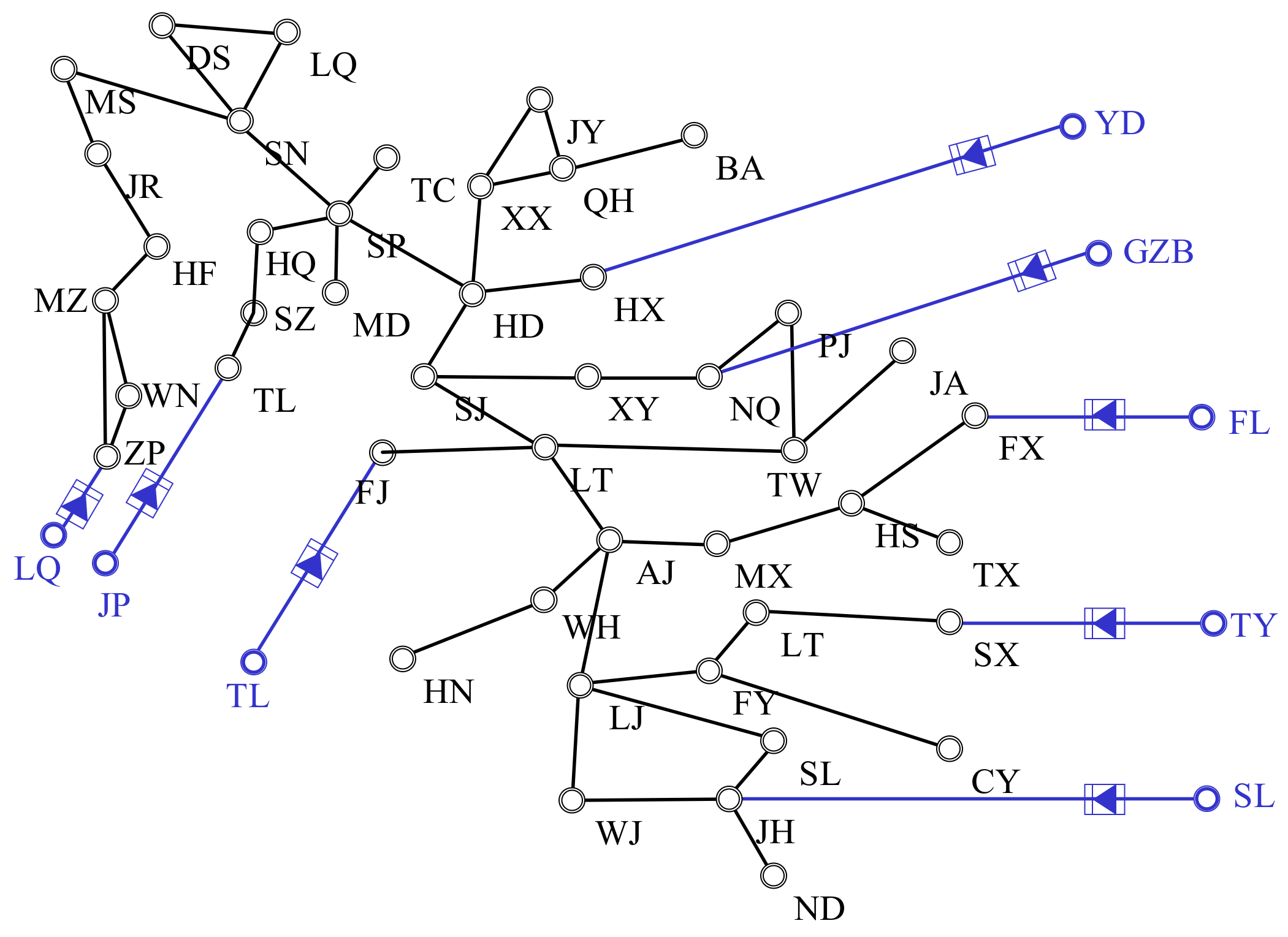
Table A2.
Corresponding parameters of the East China Power Grid.
Table A2.
Corresponding parameters of the East China Power Grid.
| Parameter | Value |
|---|---|
| Regional active load | 270 GW |
| Transmission power | 32.8 GW |
| Number of infeed DCs | 8 |
| 500 kV and above stations | 45 |
Table A3.
DC information and weight coefficient.
Table A3.
DC information and weight coefficient.
| Start Point-End Point | Transmission Power/MW | Weight Coefficient |
|---|---|---|
| SL-JH | 7500 | 0.1927 |
| FL-FX | 6000 | 0.1537 |
| JP-TL | 6700 | 0.1716 |
| GZB-NQ | 1200 | 0.0223 |
| LQ-ZP | 2800 | 00717 |
| YD-HX | 2800 | 0.0717 |
| TL-FJ | 2800 | 0.0717 |
| TY-SX | 3000 | 0.0768 |
Table A4.
Parameters of DRPCE.
Table A4.
Parameters of DRPCE.
| Type | Parameter | Value |
|---|---|---|
| SVC | Filter time constant TS1 | 0.02 s |
| Maximum voltage deviation VEMA | 0.15 p.u. | |
| Continuous control gain Ksvs | 4 | |
| SCR trigger delay | 0.06 s | |
| Voltage deviation DV | 0.1 p.u. | |
| Synchronous Condenser | Kinetic energy of generator | 448.5 MWs |
| Direct axis transient reactance | 0.165 p.u. | |
| AC transient reactance | 0.317 p.u. | |
| Direct axis transient open circuit time constant | 7.46 s |
References
- Yao, L.; Wu, J.; Wang, Z.; Li, Y.; Lu, Z. Pattern Analysis of Future HVDC Grid Development. Proc. CSEE 2014, 34, 6007–6020. [Google Scholar]
- Rahimi, E.; Gole, A.M.; Davies, J.B.; Fernando, I.T.; Kent, K.L. Commutation Failure Analysis in Multi-Infeed HVDC Systems. IEEE Trans. Power Deliv. 2011, 26, 378–384. [Google Scholar] [CrossRef]
- Wei, Z.; Yuan, Y.; Lei, X.; Wang, H.; Sun, G.; Sun, Y. Direct-Current Predictive Control Strategy for Inhibiting Commutation Failure in HVDC Converter. IEEE Trans. Power Syst. 2014, 29, 2409–2417. [Google Scholar] [CrossRef]
- Zhang, K.; Cui, Y.; Yang, Z.; Feng, Y.; Zhang, Q.; Yu, Y. Analysis of the influence of synchronous condensers on receiving-end grid with multi-infeed HVDC. In Proceedings of the 2016 IEEE International Conference on Power System Technology (POWERCON), Wollongong, Australia, 28 September–1 October 2016; pp. 1–6. [Google Scholar]
- An, W.; Wei, C.Z.; Mou, M.; Huang, W.F.; Jin, X.; Ye, H. Simulation and analysis of the control and protection performance for a multi-terminal VSC-HVDC system. In Proceedings of the 13th International Conference on Development in Power System Protection 2016 (DPSP), Edinburgh, UK, 7–10 March 2016; pp. 1–4. [Google Scholar]
- Li, S.; Chen, W.; Yin, X.; Chen, D.; Teng, Y. A Novel Integrated Protection for VSC-HVDC Transmission Line Based on Current Limiting Reactor Power. IEEE Trans. Power Deliv. 2020, 35, 226–233. [Google Scholar] [CrossRef]
- Lee, C.; Shim, J.W.; Kim, H.; Hur, K. DC Power Control Strategy of MMC for Commutation Failure Prevention in Hybrid Multi-Terminal HVDC System. IEEE Access 2020, 8, 180576–180586. [Google Scholar] [CrossRef]
- Tian, H.Y.; Sng, E.K.K. A novel solution to restore a three-phase thyristor inverter from commutation failure due to voltage dip. In Proceedings of the 2004 IEEE 35th Annual Power Electronics Specialists Conference (IEEE Cat. No.04CH37551), Aachen, Germany, 20–25 June 2004; pp. 906–912. [Google Scholar]
- Nayak, O.B.; Gole, A.M.; Chapman, D.G.; Davies, J.B. Dynamic performance of static and synchronous compensators at an HVDC inverter bus in a very weak AC system. IEEE Trans. Power Syst. 1994, 9, 1350–1358. [Google Scholar] [CrossRef]
- Saichand, K.; Padiyar, K.R. Analysis of voltage stability in multi-infeed HVDC systems with STATCOM. In Proceedings of the 2012 IEEE International Conference on Power Electronics, Drives and Energy Systems (PEDES), Bengaluru, India, 16–19 December 2012; pp. 1–6. [Google Scholar]
- Aamir, A.; Qiao, L.; Guo, C.; Rehman, A.U.; Yang, Z. Impact of synchronous condenser on the dynamic behavior of LCC-based UHVDC system hierarchically connected to AC system. CSEE J. Power Energy Syst. 2019, 5, 190–198. [Google Scholar] [CrossRef]
- Zhou, S.H.; Tang, F.; Liu, D.C.; Zhang, Q.; Yin, Q. Dynamic Reactive Power Compensation Configuration Method for Reducing the Risk of Commutation Failure in Multi-infeed DC System. High Volt. Eng. 2018, 44, 3258–3265. [Google Scholar]
- Wei, Z.; Fang, W.; Liu, J. Variable Extinction Angle Control Strategy Based on Virtual Resistance to Mitigate Commutation Failures in HVDC System. IEEE Access 2020, 8, 93692–93704. [Google Scholar] [CrossRef]
- Liu, L.; Lin, S.; Liu, J.; Sun, P.; Liao, K.; Li, X.; He, Z. Analysis and Prevention of Subsequent Commutation Failures Caused by Improper Inverter Control Interactions in HVDC Systems. IEEE Trans. Power Deliv. 2020, 35, 2841–2852. [Google Scholar]
- Song, J.; Li, Y.; Zeng, L.; Zhang, Y. Review on Commutation Failure of HVDC Transmission System. Autom. Electr. Power Syst. 2020, 44, 2–13. [Google Scholar]
- Shao, Y.; Tang, Y. A Fast Assessment Method for Evaluating Commutation Failure Risk of Multi-infeed HVDC Systems. Proc. CSEE 2017, 37, 3429–3436. [Google Scholar]
- CIGRE Working Group B4.41. Systems with Multiple DC Infeed [R]; CIGRE: Paris, France, 2008. [Google Scholar]
- Bompard, E.; Napoli, R.; Xue, F. Analysis of structural vulnerabilities in power transmission grids. Int. J. Crit. Infrastruct. Prot. 2009, 2, 5–12. [Google Scholar] [CrossRef]
- Seo, J.H.; Im, C.H.; Heo, C.G.; Kim, J.K.; Jung, H.K.; Lee, C.G. Multimodal function optimization based on particle swarm optimization. IEEE Trans. Magn. 2006, 42, 1095–1098. [Google Scholar] [CrossRef]
- Wang, L.; Ali, Y.; Nazir, S.; Niazi, M. ISA Evaluation Framework for Security of Internet of Health Things System Using AHP-TOPSIS Methods. IEEE Access 2020, 8, 152316–152332. [Google Scholar] [CrossRef]
- Liu, Z.; Zhang, Q.; Wang, Y.; Dong, C.; Zhou, Q. Research on Reactive Compensation Strategies for Improving Stability Level of Sending-end of 750 kV Grid in Northwest China. Proc. CSEE 2015, 35, 1015–1022. [Google Scholar]
- Zhang, Y.; Han, D.; Liu, W. Comprehensive Optimization of Static/Dynamic Reactive Power for Receiving-end Network. Power Autom. Equip. 2009, 29, 32–35. [Google Scholar]


Publisher’s Note: MDPI stays neutral with regard to jurisdictional claims in published maps and institutional affiliations. |
© 2021 by the authors. Licensee MDPI, Basel, Switzerland. This article is an open access article distributed under the terms and conditions of the Creative Commons Attribution (CC BY) license (https://creativecommons.org/licenses/by/4.0/).