Article

Bayesian Updates for an Extreme Value Distribution Model of Bridge Traffic Load Effect Based on SHM Data

1
College of Construction Engineering, Jilin University, Changchun 130026, China
2
Beijing Construction Engineering Research Institute Co., Ltd., Beijing 100039, China
*
Author to whom correspondence should be addressed.
Sustainability 2021, 13(15), 8631; https://doi.org/10.3390/su13158631
Submission received: 4 July 2021 / Revised: 26 July 2021 / Accepted: 29 July 2021 / Published: 2 August 2021
(This article belongs to the Special Issue Structural Health Monitoring in Civil Infrastructure)

Abstract

:
As the distribution function of traffic load effect on bridge structures has always been unknown or very complicated, a probability model of extreme traffic load effect during service periods has not yet been perfectly predicted by the traditional extreme value theory. Here, we focus on this problem and introduce a novel method based on the bridge structural health monitoring data. The method was based on the fact that the tails of the probability distribution governed the behavior of extreme values. The generalized Pareto distribution was applied to model the tail distribution of traffic load effect using the peak-over-threshold method, while the filtered Poisson process was used to model the traffic load effect stochastic process. The parameters of the extreme value distribution of traffic load effect during a service period could be determined by theoretical derivation if the parameters of tail distribution were estimated. Moreover, Bayes’ theorem was applied to update the distribution model to reduce the statistical uncertainty. Finally, the rationality of the proposed method was applied to analyze the monitoring data of concrete-filled steel tube arch bridge suspenders. The results proved that the approach was convenient and found that the extreme value distribution type III might be more suitable as the traffic load effect probability model.

1. Introduction

Bridge safety has become a public concern after several collapses in recent years [1,2]. Nowadays, increased axle load and growth of traffic density are the main causes of bridge accidents worldwide [3,4,5,6]. The actual loads on trucks are often illegally overloaded, which has led to higher risks [7]. There is an increasing demand for a systematic and efficient safety assessment of bridges to prevent possible disasters [8,9,10,11].
Among all the load effects that must be determined for a bridge assessment, the most variable effect is that induced by traffic load [12]. The accuracy of bridge safety assessments greatly depends on the accuracy of the traffic load effect probability model which describes the uncertainty of the traffic load effect [13,14]. Therefore, an accurate prediction method for an extreme traffic load effect model is desired, especially for evaluating the safety of existing bridge structures [12,15].
Traditionally, the traffic load effect probability model has been determined based on statistical regularity from conservative design code [13,16]. However, this approach neglects site-specific truck loads that may be substantially different from bridge to bridge and are important for the safety evaluation of an existing bridge [17,18]. In recognition of this, many studies have been conducted to improve the measurement of the site-specific traffic load. One of the most effective methods is the weigh-in-motion (WIM) technology [19,20,21], while others have tried to obtain traffic load effects directly through structural health monitoring (SHM) technology [22,23,24,25].
The WIM and SHM technologies solve the problem of data acquisition for site-specific traffic. It is very difficult, however, to collect enough data in a correspondingly shorter monitoring period which can be used to determine the characteristic values of extreme load effect expected over the lifetime of the design service [26,27]. Therefore, using limited data to predict extreme value distribution is a common practice [12].
Many approaches have been put forward for predicting the probability model of extreme traffic load effect based on limited site-specific data, such as the normal probability paper method and the Monte Carlo method [28]. To deal with the statistics of extremes, the extreme value theory (EVT) [29] represents an ideal framework, which has already been used for the purpose of structural dynamics [11]. The EVT has also been used for modeling extreme traffic load effect for several years. Many studies have tried to solve the problem by identifying the maximum load effect recorded during a loading event, or in a reference period such as one day or one month, and then fitting those maxima to an extreme value distribution [26]. Caprani et al. [30] classified the loading events by the number of trucks involved in the maximal load effect, and then the maxima of each loading event was modeled by the generalized extreme value (GEV) distribution.
In theory, it is not very difficult to predict the probability model for extreme value traffic load effects if they follow some common distribution types or are identically distributed. However, in practice, the distribution function of the traffic load effect is always unknown or follows a very complicated distribution, which makes the accurate estimation of extreme traffic load effect almost impossible [12,14,31]. Caprani et al. [30] highlighted that the traffic load effect is not identically distributed, which violates the assumption of classical EVT that the underlying distribution should be identically and independently distributed. According to the EVT, the tails of the probability distribution for the traffic load effect govern the behavior of extreme values [32,33]. Upon noticing this, some methods tried to solve the problem by fitting the tail data only. For example, the peaks-over-threshold (POT) [34] and generalized Pareto distribution (GPD) estimation [35]. Regardless of the POT method or the GPD estimation, they are both sensitive to the threshold, but a relatively high threshold will increase the statistical uncertainty of estimated extreme value [36].
As a result, the statistical uncertainty of probability distribution parameters cannot be ignored [33]. Meanwhile, the traffic load conditions will change during the bridge operation period, so the traffic load effect model should also be updated to reflect the real status of traffic. To solve this problem, the Bayesian approach may offer an appealing alternative [4,37]. The Bayesian approach has been utilized to estimate the extreme value of bridges due to various loads. Sheng Xu et al. [36] proposed the Bayesian method to study the short-term extreme mooring tensions. Y.Q Ni et al. applied the Bayesian approaches when evaluating the wind-resistant performance [38] and condition assessment [39]. Yiming Gu et al. [14] proposed a novel Bayesian approach for estimating the extreme traffic. Most of the above research does not pay attention to the stochastic process, while some is under the framework of Gaussian processes [11,40]. According to the Unified Standard for Reliability Design of Highway Engineering Structures (GB/T 50283-1999), the traffic loading process conforms to a filtered Poisson process (FPP). The character of the FPP will influence which extreme value distribution model of traffic load effect is needed.
The purpose of this study is to introduce a method for predicting the probability model of extreme traffic load effect based on SHM data. To establish the value distribution of extreme traffic load effect, the method uses a generalized Pareto distribution (GPD). This models the tail distribution of traffic load effect based on the POT method and FPP, which is based on the EVT for stochastic processes. Meanwhile, since the number of extreme traffic load effect values in the sample is relatively small, especially when the threshold is high [36,39], the Bayes’ theorem is applied to reduce the statistical uncertainty and update the distribution model.

2. Modeling Method for Extreme Traffic Load Effect

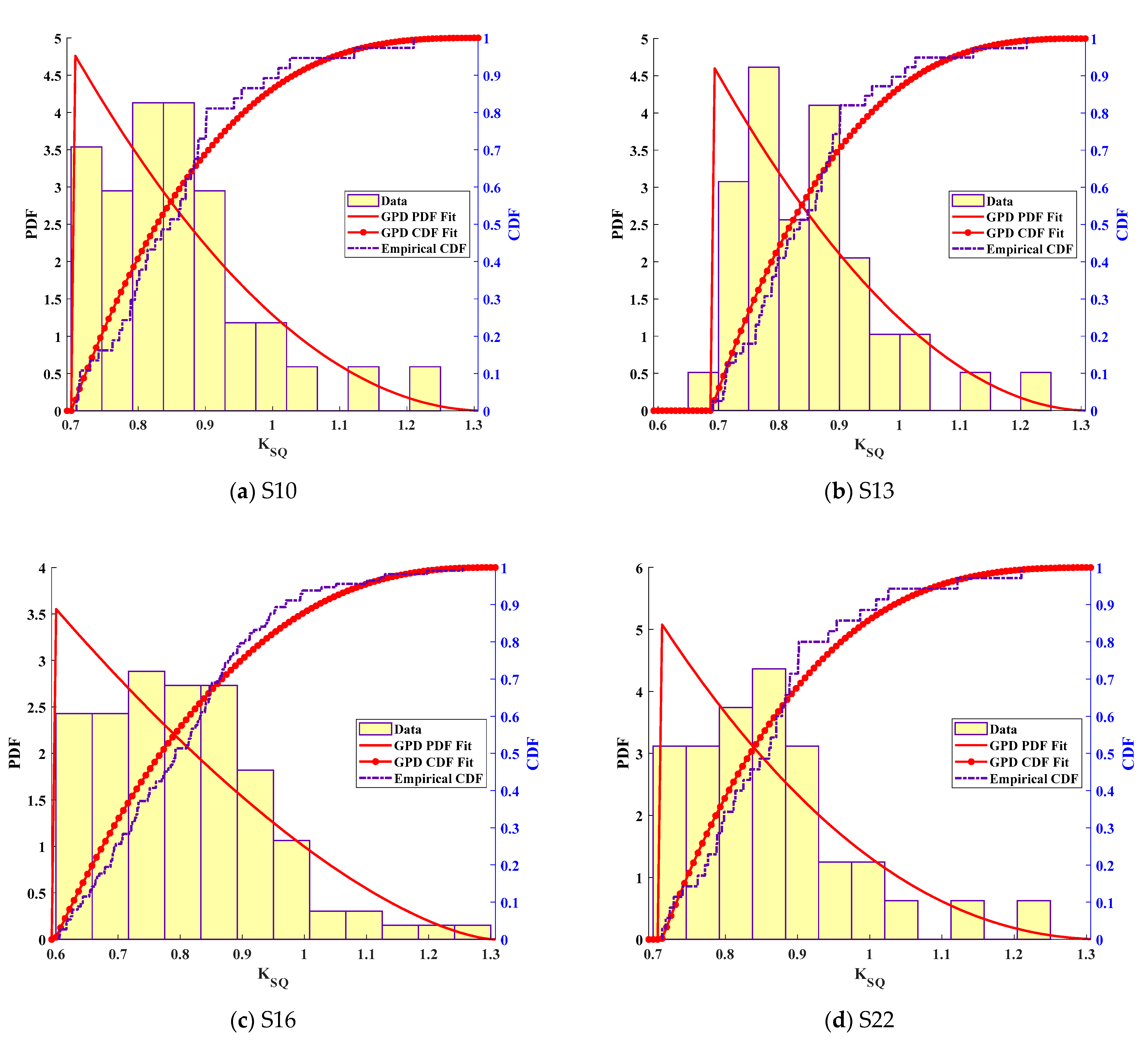
2.1. The GPD Model for Peaks-Over-Threshold Traffic Load Effect

To model the tail distribution, the POT method is applied to treat the POT traffic load effect data.
The POT method is a natural choice for modeling exceedance over a threshold. It has shown its importance and success in a number of statistical analysis areas such as finance, insurance, hydrology, and geographical phenomena domains [14,41,42], and in recent years, it has attracted attention for modeling extreme values of bridge traffic load effect.
Traditionally, traffic load effect caused by trucks crossing a bridge has been assumed to be a sequence of independent and identically distributed observations, i.e., s 1 ,     s 2 ,   ,   s n , with the same marginal distribution function, F s ( ) . Therefore,   s m a x denotes its extreme value as follows:
S m a x = max ( s 1 , s 2 , ,   s n )
In theory, the distribution of S m a x can be derived exactly as Equation (2), if F s ( ) is known:
F S m a x ( s m a x ) = P { S m a x s } = P { max ( s 1 , s 2 , s n ) s } = P { s 1 s , s n s } = F s n ( s )
Most of the time, however, the distribution function, F s ( ) , is unknown. In this case, the distribution F s n ( s ) can be approximated by the GEV distribution according to the EVT.
F s n ( s ) H ( x ; μ ˜ , σ ˜ , ξ ˜ ) = e x p { ( 1 + ξ ˜ x μ ˜ σ ˜ ) 1 / ξ } , 1 + ξ ˜ x μ ˜ σ ˜ > 0
where  μ ˜ , σ ˜ , and ξ ˜ are the location, scale, and shape parameters of GEV distribution, respectively. Although the GEV model can be used to describe the probability model of s m a x , the problem of how to define the values of μ ˜ , σ ˜ , ξ ˜ remains, since the extreme data s m a x is limited most of the time.
The extreme traffic load effect, s m a x , is the maximum value of s 1 , s 2 , , s n and it is also the maximum value of s * , which is the traffic load effect in s 1 , s 2 , ,   s n that exceeds the high threshold  u . The probability distribution function of s * can be defined by the conditional probability in the POT method, as Equation (4):
{ F s * ( s * ) = F s ( s * ) F s ( u ) 1 F s ( u )         s * u F s * ( s * ) = 0                                           s * < u
According to the EVT, the previous distribution, F s * ( s * ) , belongs to the GPD family if the threshold u is large enough. The GPD, which has been proven to be the limit distribution of scaled excess over high threshold values, is often used to fit the upper tail of the probability distribution [33].The cumulative distribution function (CDF) of the GPD is defined as follows:
G ( x ; μ , σ , ξ ) = 1 ( 1 + ξ x μ σ ) 1 / ξ x μ ,       1 + ξ x μ σ > 0 μ = u
where μ , σ , and ξ are the location, scale, and shape parameters of GPD, respectively.

2.2. The Filtered Poisson Process Model for the Traffic Load Effect Stochastic Process

The traffic loading process is a stochastic process which conforms to an FPP. Since the traffic load and its load effect usually have a linear relationship, the traffic load effect process, S ( t ) , can also be reasonably defined as an FPP (Equation (6)):
{ S ( t ) = n = 0 N ( t ) ω ( t , τ i , s i ) ,       t 0 ω ( t , τ i , s i ) = { s i ,       t τ i 0 ,       t τ i ,   i = 0 , 1 , 2
where { N ( t ) , t 0 } is the number of traffic load effects during period t , which follows the Poisson process with parameter λ ; s i is the i -th traffic load effect according to the appearance time, which is an identically and independently distributed random variable with F s ( s ) as CDF; τ i is the time when s i appears.
Compared with the traffic load effect process S ( t ) , the stochastic process model of the traffic load effect which exceeds a high threshold S * ( t ) can be reasonably defined as an FPP, but with different parameters (Equation (7)):
{ S * ( t ) = n = 0 N * ( t ) ω * ( t , τ i , s i * ) , t 0 ω * ( t , τ i * , s i * ) = { s i * ,       t τ i * 0 ,       t τ i * , i = 0 , 1 , 2
where s i * is the i -th traffic load effect over a high threshold u according to the appearance time with F s * ( s * ) as CDF; N * ( t ) is the number of s i * during the period t , and the Poisson process with parameter λ * = [ 1 F s ( s γ ) ] λ .

2.3. Probability Model for Extreme Traffic Load Effect

According to the EVT, the CDF of the traffic load effect EV distribution for an FPP during the service period T is as follows:
F s m a x ( s m a x ) = e x p { λ T [ 1 F s ( s m a x ) ] }
For the same reason, the CDF of a traffic load effect that exceeds a high threshold EV distribution for an FPP during the service period T is as follows:
{ F s m a x * ( s m a x ) = e x p { λ * T [ 1 F s * ( s m a x ) ] } λ * = [ 1 F s ( s γ ) ] λ
With Equations (4), (8), and (9), Equation (10) can be deduced as follows:
F s m a x * ( s m a x ) = e x p { λ T [ 1 F s ( s m a x ) ] } = F s m a x ( s m a x )
Equation (10) proves the equivalence between F s m a x * ( s m a x ) and F s m a x ( s m a x ) , which means the probability model of extreme traffic load effect can be obtained through the analysis of the traffic load effect that exceeds a high threshold.
As mentioned in Section 2.1, the probability model of peak-over-threshold traffic load effect, F s * ( s * ) , follows a GPD. With Equations (5) and (9), the CDF of the traffic load effect that exceeds a high threshold EV distribution for an FPP during the service period T is Equation (11), which obviously follows the GEV distribution:
{ F s m a x * ( s m a x ) = e x p { ( 1 + ξ ˜ s m a x μ ˜ σ ˜ ) 1 / ξ ˜ } μ ˜ = μ σ [ 1 ( λ * T ) ξ ] ξ 1 σ ˜ = σ ( λ * T ) ξ ξ ˜ = ξ

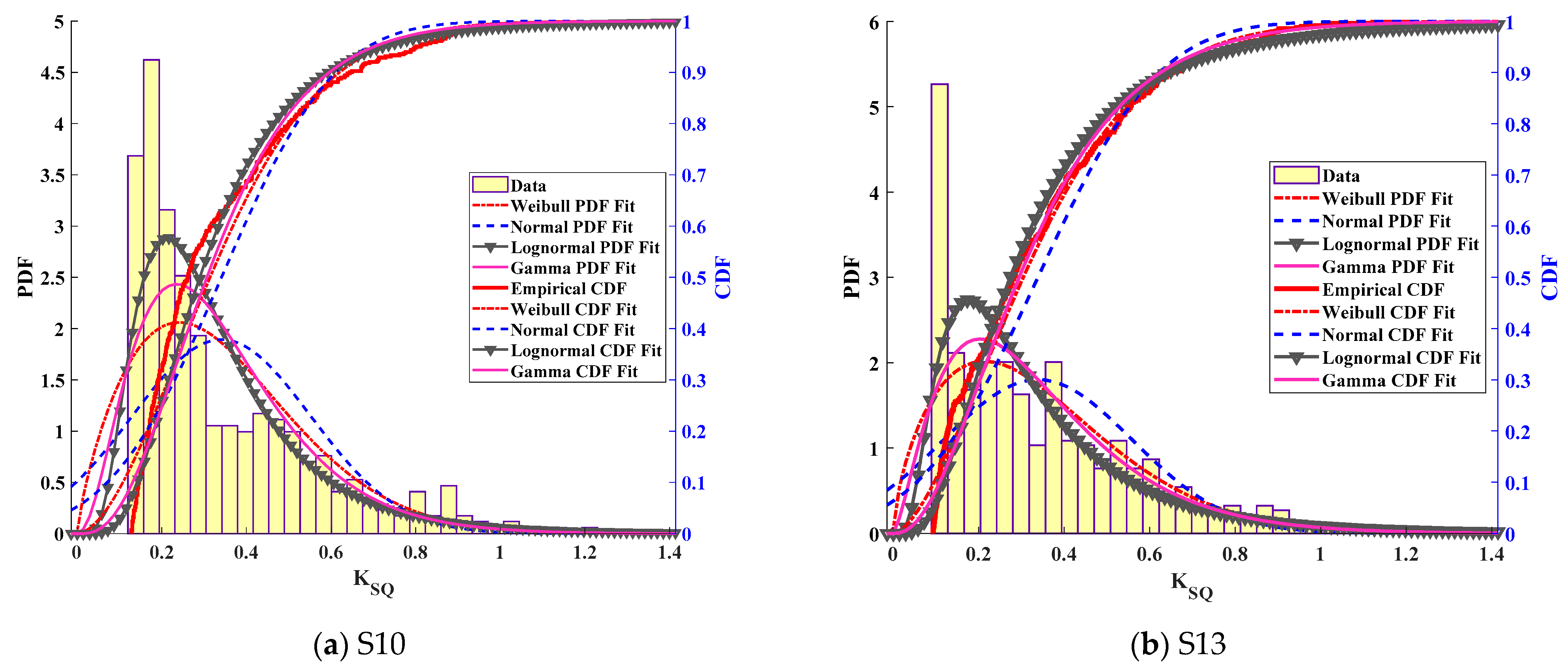
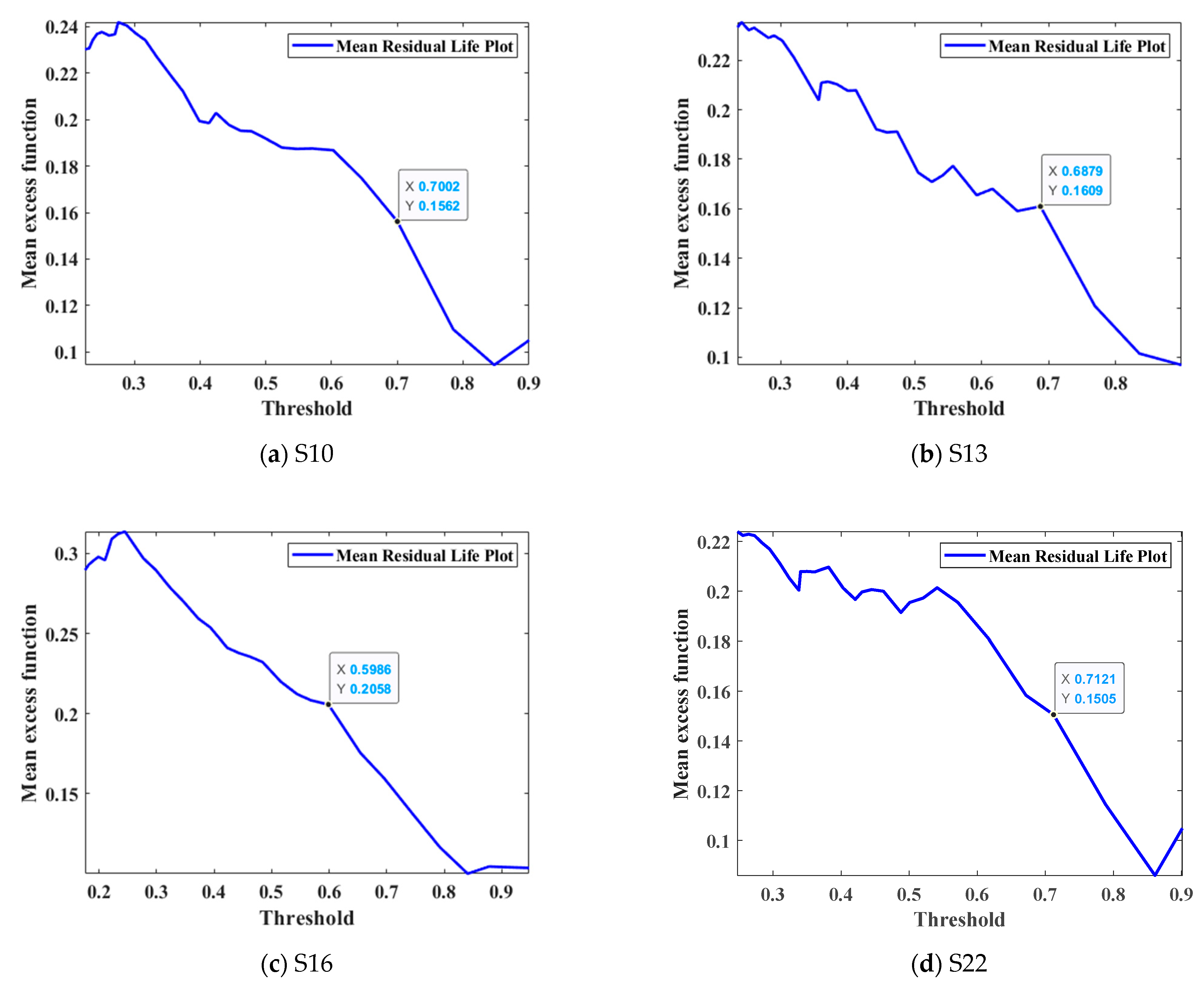
2.4. Parameter Estimation Based on Bridge Health Monitoring Data

Equation (11) tells us if the distribution parameters of the traffic load effect that exceeds a high threshold can be determined; therefore, the probability model of extreme traffic load effect is established.
Threshold selection is an important step in the application of the POT method. An appropriate threshold is critical for estimating the EV distribution [33,43]. To choose an appropriate threshold, the mean excess function (MEF) [44] of the GPD is defined as follows:
e n ( μ ) = E ( X μ | X > μ ) = σ + ξ μ 1 ξ
Therefore, e n ( μ ) is a linear function of μ and E ( X μ | X > μ ) is simply the mean of the exceedances of the threshold μ . According to Equation (12), the sample estimator of e n ( μ ) is as follows:
e n ( μ ) = 1 n i = 1 n ( x i μ )
where x i consists of the n observations that exceed μ . If the exceedance of the threshold μ = u 0 , the MEF of the samples over u 0 will produce a straight line, or close to it. The point set { μ , e n ( μ ) } is considered to be the mean residual life plot (MRLP). The MRLP provides a valid approximation of the distribution of the exceedances. If the threshold u 0 is appropriate, the μ > u 0 region of the MRLP is nearly a straight line.
After determining the threshold μ , the parameters of the GPD can be estimated by maximum likelihood. Supposing the values x 1 ,   ,   x k are the k exceedances of a threshold u 0 , for ξ 0 the log-likelihood is derived as follows:
l ( σ , ξ ) = k log σ ( 1 + 1 ξ ) i = 1 k log ( 1 + ξ x i σ )
In the case ξ = 0 , the log-likelihood is obtained as follows:
l ( σ , ξ ) = k log σ σ 1 i = 1 k x i
The values x 1 ,   ,   x k are obtained from the bridge health monitoring data. Analytical maximization of the log-likelihood is not possible; therefore, numerical techniques are again required. Standard errors and confidence intervals for the GPD are obtained from standard likelihood theory.
According to the bridge health monitoring data, the parameter λ * can be determined as follows:
λ * = n t Δ t
where   n t is the number of data that exceed the threshold u 0 during a monitoring period Δ t , which reflects the traffic volume changes at different sites during different periods of service.
Since the existing bridge structure has been in service for a few years, there are some differences between T for the existing bridge structure and the design reference period T N for the new bridge structure, which need to be considered. To determine T , the equal exceeding probability principle [45] is applied and T can be calculated as follows:
T = M N · T N
where M represents the remaining design working life for the existing bridge and N represents the design working life.

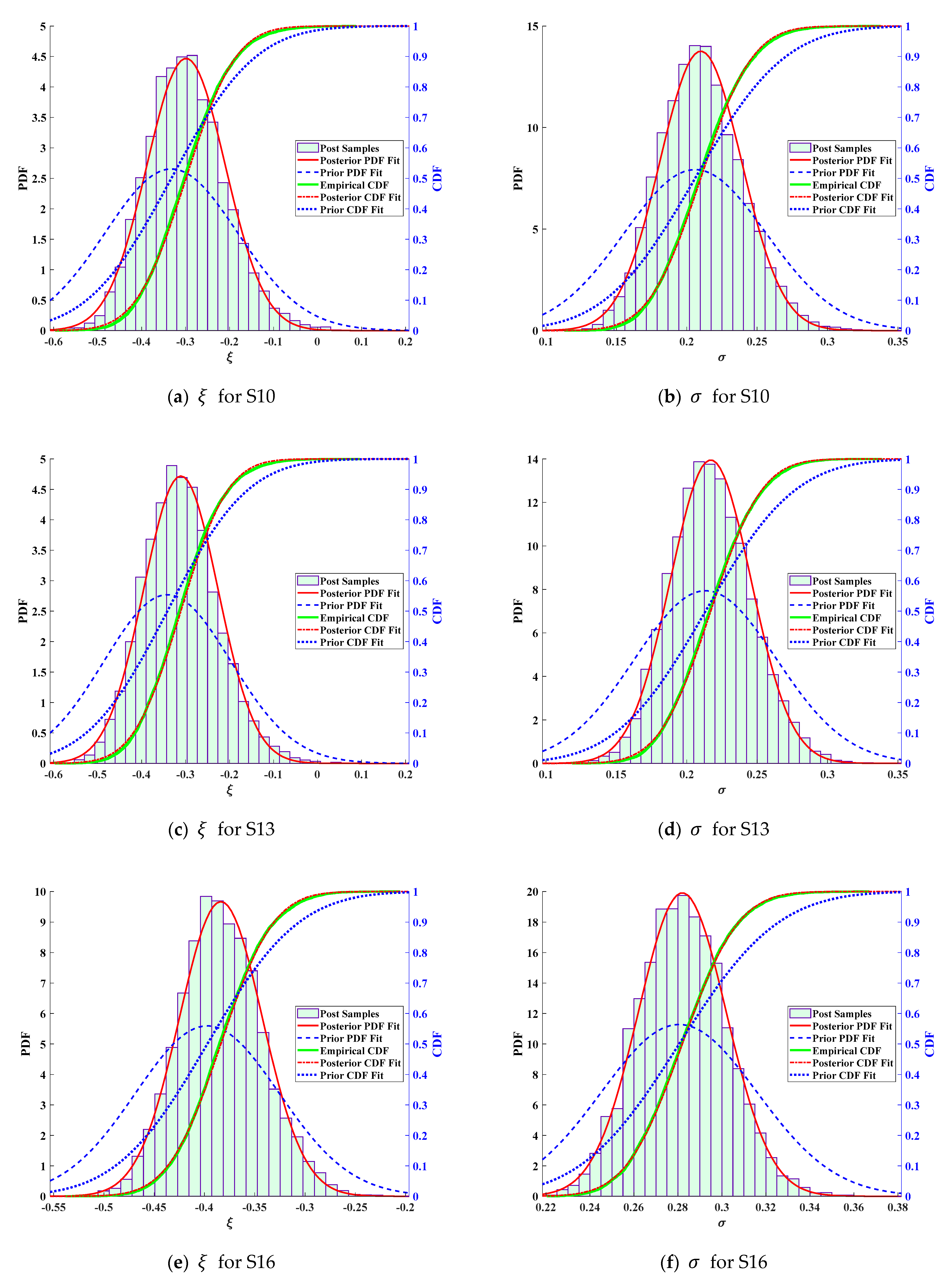
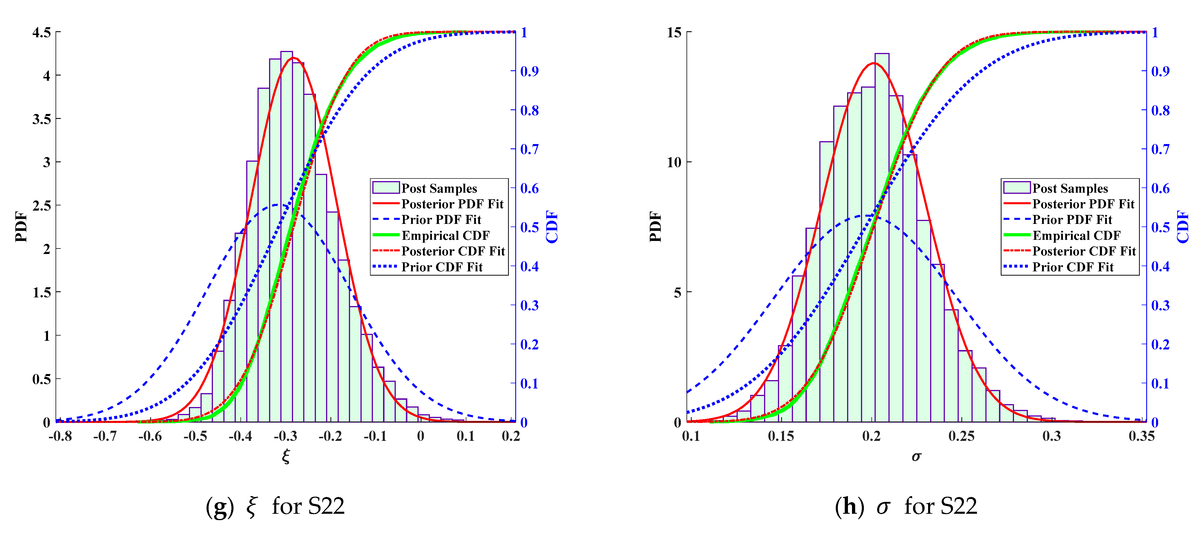
3. Bayesian Updates for the Extreme Traffic Load Effect Model

The number of traffic load effect extreme value samples is relatively small, especially when the threshold is high. As a result, the statistical uncertainty of probability distribution parameters cannot be ignored. Meanwhile, the traffic load conditions will change during the bridge operation period, meaning the traffic load effect model should also be updated to reflect the real status of traffic. In this paper, a Bayesian approach is employed to update the extreme traffic load effect based on monitoring data.
In general, Bayes’ theorem can be expressed in terms of probability density function (PDF) as follows:
π ( θ | x ) = L ( x | θ ) π ( θ ) Θ L ( x | θ ) π ( θ ) d θ
where π ( θ ) is the prior distribution of the model parameters θ (e.g., σ   and   ξ in GPD) and Θ  is the parameter space. π ( θ ) represents the statistical uncertainty which can be decreased as additional traffic load effect monitoring data x are gathered, π ( θ | x )  is the posterior distribution of θ and represents the updated conditions of θ , and L ( x | θ ) is the likelihood function.
The marginal likelihood of x can be expressed as follows:
m ( x ) = Θ L ( x | θ ) π ( θ ) d θ
Therefore, the posterior distribution π ( θ | x ) expression is shortened as follows:
π ( θ | x ) L ( x | θ ) π ( θ )
On the basis of the above Bayes’ theorem, the updated Bayesian procedure for the extreme traffic load effect model is as follows:
  • Evaluate π ( θ )
    Since the GEV distribution parameters can be calculated by GPD distribution parameters (see Equation (11)), only σ   and   ξ need to be chosen as the model parameters θ . At the beginning, several methods can be used to evaluate the original π ( θ ) , such as Jeffreys prior of flat priors, even if no monitoring data are obtained. When the new monitoring data x are gathered, the previous posterior distribution π ( θ | x ) becomes the new priors.
  • Evaluate π ( θ | x )
    It is very difficult to evaluate π ( θ | x ) by direct numerical integration, but the Markov Chain Monte Carlo (MCMC) algorithm provides a good solution to this problem. The basic idea of the MCMC algorithm is to simulate the Markov Chain, whose stationary distribution is π ( θ | x ) . Next, π ( θ | x ) can be sampled based on the stationary distribution.
  • Model update
    The posterior distribution, π ( θ | x ) , contains the information from the new data x and also the prior information from π ( θ ) . Therefore, the mean values of π ( θ | x ) are chosen as the updated model of parameters  θ .

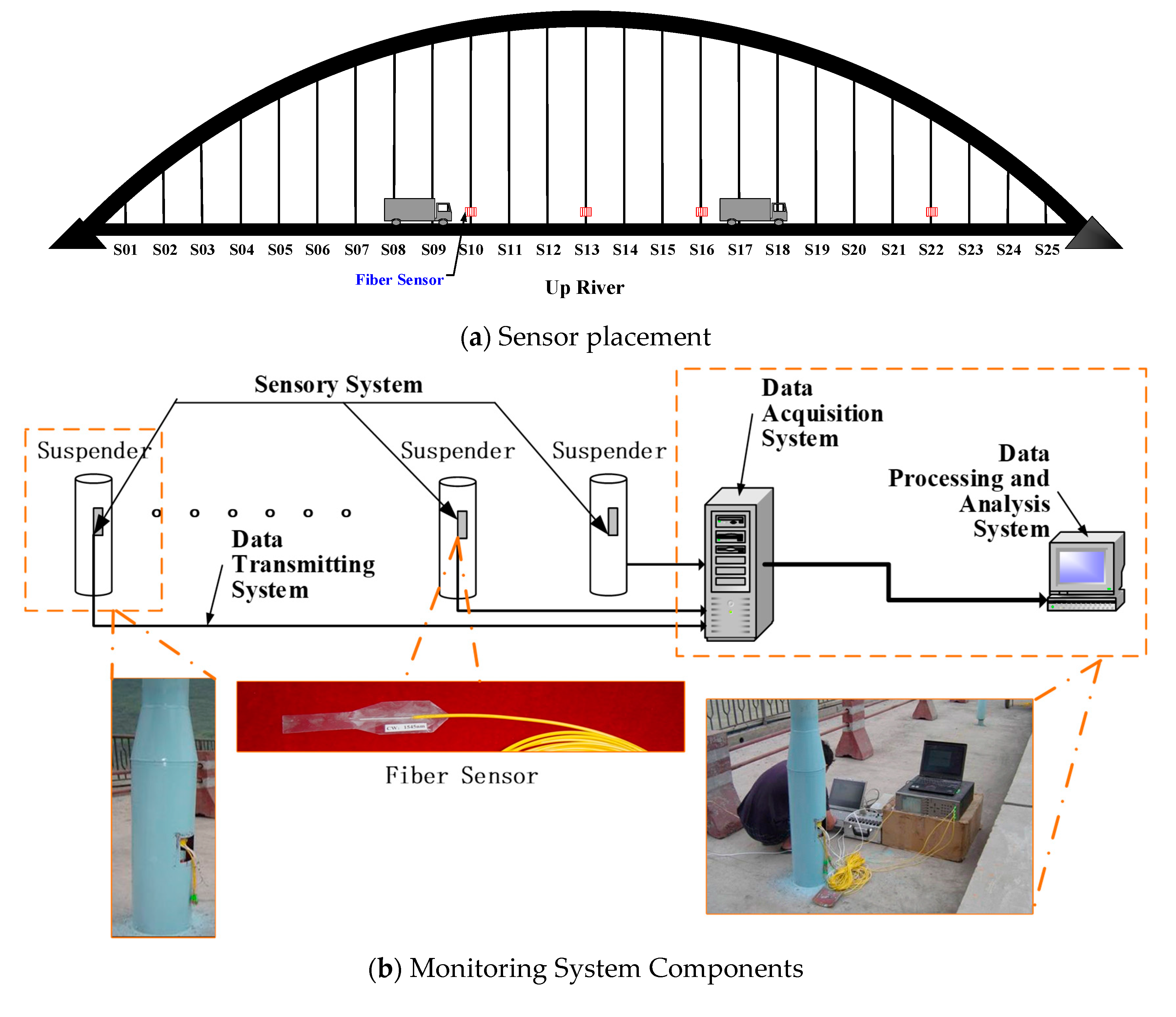
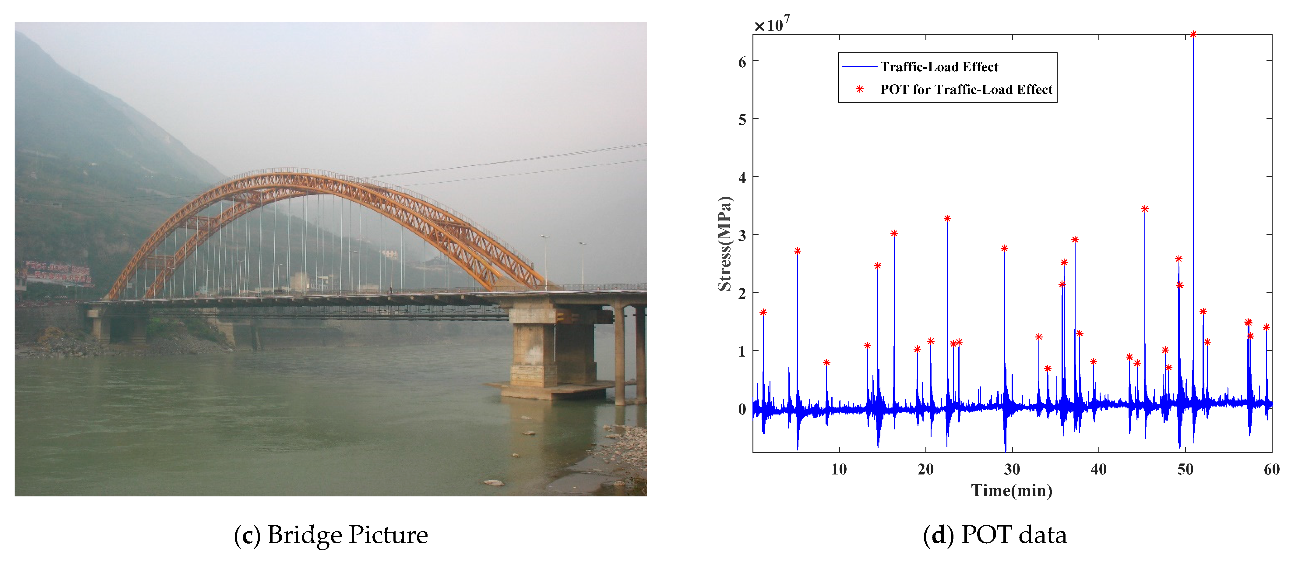
4. Application to a CFST Arch Bridge

In recent years, several through and half-through arch bridge collapsing accidents have happened in China. Most of those accidents were caused by broken suspenders. The increasing traffic load was a primary cause of the suspender breakage, such that the analysis of traffic load effect probabilistic models of suspenders has become a research focus [46].
The E’Bian bridge, as shown in Figure 1, is a half-through concrete-filled steel tube (CFST) arch bridge located in China. The main span is 138 m and the width is 13 m. The arch rib is made of CFST with 50 suspenders connected to the concrete deck. A vehicle load effect monitoring system was implemented on suspenders on this bridge, as shown in Figure 1. The monitoring system can collect the traffic load effect data through the fiber sensor installed on the steel wires of the suspenders (Figure 1).
Figure 2 illustrates the distribution of traffic load effect on four suspenders (S10, S13, S16, and S22). KSQ = SQ/SK, where SQ is the real stress on the suspender steel wires and SK is the normal value of the traffic load effect calculated by the design code. It can be observed in Figure 2 that the Weibull distribution, normal distribution, log-normal distribution, and gamma distribution, which are recommended in the Unified Standard for Reliability Design of Highway Engineering Structures (GB/T 50283-1999) as the traffic load effect model, deviate from the empirical distribution for the multi-peak phenomenon.
As the probability model recommended by the design code does not properly satisfy the result, a tail-based model is employed. First, a threshold is determined by inspecting the MRLP, as shown in Figure 3. The threshold for each suspender is chosen at the point where the MRLP becomes almost a straight line. Then, based on the standard likelihood theory, the tail region data can be fitted by the GPD (Figure 4), which is accepted by the K–S test.
The priors for GPD parameters σ   and   ξ are assumed to follow a normal distribution in this study, and the hyper parameters μ σ ,   σ σ , and μ ξ ,   σ ξ can be generated from the prior monitoring data as follows:
σ ~ N ( μ σ , σ σ ) ,     ξ ~ N ( μ ξ , σ ξ )
When new monitoring data are obtained, the MCMC algorithm is used to evaluate π ( θ | x ) based on the new monitoring data x . Then, the samples of π ( θ | x ) are generated and the model parameters of π ( θ | x ) are found by likelihood estimation. In this study, the new monitoring data are simulated based on the prior GPD model to show the updated effect. The results (See Figure 5) clearly show that the variance of θ is reduced after updating.
For a suspender, if the design working life, N, is 30 years, the remaining design working life, M, is 6 years, and the design reference period, TN, is 100 years, according to Equation (17), the reference period, T, for the suspenders is 20 years. The probability model of extreme traffic load effect for the suspenders, the mean, and the standard deviation (S.D.) of x u p based on the above parameters, are shown in Table 1.

5. Discussion

There is an interesting result that should be discussed. The parameter ξ ˜ in GPD and GEV is negative, which means the extreme traffic load effect probability model follows the extreme value distribution type III (Weibull families). Bailey and Bez [18] reached a similar conclusion from the simulated static effects of traffic, but they require more proof. According to the EVT, if ξ ˜ or ξ < 0 , the GPD and GEV have an upper bound of the distribution equal to the following:
x u p = μ ˜ σ ˜ ξ ˜ = μ σ [ 1 ( λ * T ) ξ ] ξ 1 σ ( λ * T ) ξ ξ 1 = μ σ ξ
According to the Unified Standard for Reliability Design of Highway Engineering Structures (GB/T 50283-1999), the extreme traffic load effect probability model is usually assumed to be a normal distribution or extreme value distribution type I, which does not have an upper bound. In general, the traffic load effect cannot be unlimited if there is no damage where the monitoring sensor is placed. This means the extreme value distribution type III might be more reasonable as the probability model for the extreme traffic load effect, compared with the conventional models.

6. Conclusions

In this study, an updated Bayesian approach for predicting the extreme value distribution of traffic load effect using monitoring data is proposed based on the EVT for stochastic processes. The following conclusions can be made:
(I) The GPD is suitable for modeling the tail distribution of traffic load effect data. This solves the problem of the distribution of actual traffic load effect, which sometimes follows uncommon types of probability distribution. As such, conventional methods cannot accurately predict the probability model of extreme traffic load effect using bridge structure health monitoring data.
(II) The extreme traffic load effect excess for an FPP during a service period is proven to follow the GEV distribution, when the probability model of peak-over-threshold traffic load effect follows the GPD.
(III) Bayesian updates can reduce the variance of distribution model parameters θ .
(IV) The improved method can consider the site-specific features of traffic load and also the differences between T for an existing bridge structure and the design reference period, T N , for a new bridge structure.
(V) The application results show that the extreme value distribution of traffic load effect follows the extreme value distribution type III (Weibull families), which has an upper bound and might be more reasonable than the conventional model.
(VI) Threshold selection is an important step in the application of the new method. An appropriate threshold is critical for estimating the EV distribution. Although the mean residual life plot presents a typical graphical method, it is not accurate enough. How to estimate a proper threshold should be addressed in future studies.
(VII) Other than the traditional standard likelihood theory, many methods such as the differential evolution algorithm [47] can be used to estimate the parameters of GDP based on monitoring data, and can be studied in the future.

Author Contributions

Conceptualization, X.G.; methodology, X.G.; formal analysis, X.G. and G.D; investigation, X.G., G.D., and C.L.; data curation, G.D. and C.L.; writing—original draft preparation, X.G., G.D., and C.L.; writing—review and editing, X.G., G.D., and C.L.; supervision, X.G. and C.L.; funding acquisition, X.G. and C.L. All authors have read and agreed to the published version of the manuscript.

Funding

This research was funded by the National Natural Science Foundation of China, grant number 51208224.

Institutional Review Board Statement

Not applicable.

Informed Consent Statement

Not applicable.

Data Availability Statement

The data collected are original and specific to the research. Data are available from the corresponding author upon request.

Conflicts of Interest

The authors declare no conflict of interest.

References

  1. Flint, M.M.; Fringer, O.; Billington, S.L.; Freyberg, D.; Diffenbaugh, N.S. Historical Analysis of Hydraulic Bridge Collapses in the Continental United States. J. Infrastruct. Syst. 2017, 23, 4017005. [Google Scholar] [CrossRef] [Green Version]
  2. Xu, F.Y.; Zhang, M.J.; Wang, L.; Zhang, J.R. Recent Highway Bridge Collapses in China: Review and Discussion. J. Perform. Constr. Facil. 2016, 30, 4016030. [Google Scholar] [CrossRef]
  3. Leahy, C.; Obrien, E.; O’Connor, A. The Effect of Traffic Growth on Characteristic Bridge Load Effects. Transp. Res. Procedia 2016, 14, 3990–3999. [Google Scholar] [CrossRef] [Green Version]
  4. Strauss, A.; Frangopol, D.M.; Kim, S. Use of monitoring extreme data for the performance prediction of structures: Bayesian updating. Eng. Struct. 2008, 30, 3654–3666. [Google Scholar] [CrossRef]
  5. Frangopol, D.M.; Strauss, A.; Kim, S. Use of monitoring extreme data for the performance prediction of structures: General approach. Eng. Struct. 2008, 30, 3644–3653. [Google Scholar] [CrossRef]
  6. Lei, X.; Sun, L.; Xia, Y.; He, T. Vibration-Based Seismic Damage States Evaluation for Regional Concrete Beam Bridges Using Random Forest Method. Sustainability 2020, 12, 5106. [Google Scholar] [CrossRef]
  7. Fu, G.; You, J. Truck Loads and Bridge Capacity Evaluation in China. J. Bridge Eng. 2009, 14, 327–335. [Google Scholar] [CrossRef]
  8. Xia, M.; Cai, C.S.; Pan, F.; Yu, Y. Estimation of extreme structural response distributions for mean recurrence intervals based on short-term monitoring. Eng. Struct. 2016, 126, 121–132. [Google Scholar] [CrossRef]
  9. Deng, Y.; Phares, B.M. Automated bridge load rating determination utilizing strain response due to ambient traffic trucks. Eng. Struct. 2016, 117, 101–117. [Google Scholar] [CrossRef] [Green Version]
  10. Sung, Y.-C.; Lin, T.-K.; Chiu, Y.-T.; Chang, K.-C.; Chen, K.-L.; Chang, C.-C. A bridge safety monitoring system for prestressed composite box-girder bridges with corrugated steel webs based on in-situ loading experiments and a long-term monitoring database. Eng. Struct. 2016, 126, 571–585. [Google Scholar] [CrossRef]
  11. Martucci, D.; Civera, M.; Surace, C. The Extreme Function Theory for Damage Detection: An Application to Civil and Aerospace Structures. Appl. Sci. 2021, 11, 1716. [Google Scholar] [CrossRef]
  12. Zhou, X.-Y.; Schmidt, F.; Toutlemonde, F.; Jacob, B. A mixture peaks over threshold approach for predicting extreme bridge traffic load effects. Probabilistic Eng. Mech. 2016, 43, 121–131. [Google Scholar] [CrossRef] [Green Version]
  13. Obrien, E.J.; Schmidt, F.; Hajializadeh, D.; Zhou, X.-Y.; Enright, B.; Caprani, C.C.; Wilson, S.; Sheils, E. A review of probabilistic methods of assessment of load effects in bridges. Struct. Saf. 2015, 53, 44–56. [Google Scholar] [CrossRef] [Green Version]
  14. Gu, Y.; Li, S.; Li, H.; Guo, Z. A novel Bayesian extreme value distribution model of vehicle loads incorporating de-correlated tail fitting: Theory and application to the Nanjing 3rd Yangtze River Bridge. Eng. Struct. 2014, 59, 386–392. [Google Scholar] [CrossRef]
  15. Caprani, C.C.; Obrien, E.J.; Lipari, A. Long-span bridge traffic loading based on multi-lane traffic micro-simulation. Eng. Struct. 2016, 115, 207–219. [Google Scholar] [CrossRef]
  16. Nowak, A.S.; Szerszen, M.M. Bridge load and resistance models. Eng. Struct. 1998, 20, 985–990. [Google Scholar] [CrossRef]
  17. Nowak, A.S.; Ferrand, D.M. Truck Load Models for Bridges. In Building on the Past: Securing the Future (Proceeding of the 2004 Structures Congress); George, E.B., Ed.; ASCE: Nashville, TN, USA, 2004; Volume 137, p. 122. [Google Scholar]
  18. Bailey, S.F.; Bez, R. Site specific probability distribution of extreme traffic action effects. Probabilistic Eng. Mech. 1999, 14, 19–26. [Google Scholar] [CrossRef]
  19. O’Connor, A.; O’Brien, E.J. Traffic load modelling and factors influencing the accuracy of predicted extremes. Can. J. Civ. Eng. 2005, 32, 270–278. [Google Scholar] [CrossRef] [Green Version]
  20. Miao, T.; Chan, T.H.T. Bridge live load models from WIM data. Eng. Struct. 2002, 24, 1071–1084. [Google Scholar] [CrossRef]
  21. Marques, F.; Moutinho, C.; Hu, W.-H.; Cunha, Á.; Caetano, E. Weigh-in-motion implementation in an old metallic railway bridge. Eng. Struct. 2016, 123, 15–29. [Google Scholar] [CrossRef]
  22. Lan, C.; Li, H.; Ou, J. Traffic load modeling based on structural health monitoring data. Struct. Infrastruct. Eng. 2011, 7, 379–386. [Google Scholar] [CrossRef]
  23. Cao, J.; Liu, Y.; Li, C. Damage cross detection between bridges monitored within one cluster using the difference ratio of projected strain monitoring data. Struct. Health Monit. 2021. [Google Scholar] [CrossRef]
  24. Zhang, S.; Liu, Y. Damage detection of bridges monitored within one cluster based on the residual between the cumulative distribution functions of strain monitoring data. Struct. Health Monit. 2020, 19, 1764–1789. [Google Scholar] [CrossRef]
  25. Choi, Y.; Lee, J.; Kong, J. Performance Degradation Model for Concrete Deck of Bridge Using Pseudo-LSTM. Sustainability 2020, 12, 3848. [Google Scholar] [CrossRef]
  26. Zhou, X.Y.; Schmidt, F.; Jacob, B.; Toutlemonde, F. Accurate and Up-to-Date Evaluation of Extreme Load Effects for Bridge Assessment. TRA-Transp. Res. Arena 2014, 1, 1–8. [Google Scholar]
  27. Chen, S.; Wu, J. Modeling stochastic live load for long-span bridge based on microscopic traffic flow simulation. Comput. Struct. 2011, 89, 813–824. [Google Scholar] [CrossRef]
  28. Nowak, A.S. Live load model for highway bridges. Struct. Saf. 1993, 13, 53–66. [Google Scholar] [CrossRef] [Green Version]
  29. Kotz, S.; Nadarajah, S. Extreme Value Distributions: Theory and Applications; World Scientific Publishing Company: London, UK, 2000. [Google Scholar]
  30. Caprani, C.C.; Obrien, E.J.; McLachlan, G.J. Characteristic traffic load effects from a mixture of loading events on short to medium span bridges. Struct. Saf. 2008, 30, 394–404. [Google Scholar] [CrossRef]
  31. Obrien, E.J.; Enright, B.; Getachew, A. Importance of the Tail in Truck Weight Modeling for Bridge Assessment. J. Bridg. Eng. 2010, 15, 210–213. [Google Scholar] [CrossRef]
  32. Xin, G.; Lei, W. Modeling method for extreme traffic-load effect probabilistic model of an existing bridge. J. Harbin Eng. Univ. 2013, 34, 995–999. [Google Scholar]
  33. Jonathan, P.; Randell, D.; Wadsworth, J.; Tawn, J. Uncertainties in return values from extreme value analysis of peaks over threshold using the generalised Pareto distribution. Ocean Eng. 2021, 220, 107725. [Google Scholar] [CrossRef]
  34. Schmidt, F.; Zhou, X.Y.; Toutlemonde, F. A Peaks-Over-Threshold Analysis of Extreme Traffic Load Effects on Bridges. In Proceedings of the Young Research Seminar, Lyon, France, 5–7 June 2013. [Google Scholar]
  35. Ashkar, F.; El Adlouni, S.-E. Adjusting for small-sample non-normality of design event estimators under a generalized Pareto distribution. J. Hydrol. 2015, 530, 384–391. [Google Scholar] [CrossRef]
  36. Xu, S.; Soares, C.G. Bayesian analysis of short term extreme mooring tension for a point absorber with mixture of gamma and generalised pareto distributions. Appl. Ocean Res. 2021, 110, 102556. [Google Scholar] [CrossRef]
  37. Beck, J.; Katafygiotis, L. Updating Models and Their Unvertainties I: Baysian Statistical Framework. J. Eng. Mech. 1998, 1244, 455–461. [Google Scholar] [CrossRef]
  38. Wang, Y.; Ni, Y.; Zhang, Q.; Zhang, C. Bayesian approaches for evaluating wind-resistant performance of long-span bridges using structural health monitoring data. Struct. Control Health Monit. 2021, 28, e2699. [Google Scholar] [CrossRef]
  39. Ni, Y.Q.; Wang, Y.W.; Zhang, C. A Bayesian approach for condition assessment and damage alarm of bridge expansion joints using long-term structural health monitoring data. Eng. Struct. 2020, 212, 110520. [Google Scholar] [CrossRef]
  40. Clifton, D.A.; Clifton, L.; Hugueny, S.; Wong, D.; Tarassenko, L. An Extreme Function Theory for Novelty Detection. IEEE J. Sel. Top. Signal Process. 2012, 7, 28–37. [Google Scholar] [CrossRef]
  41. Cañellas, B.; Orfila, A.; Méndez, F.J.; Menéndez, M.; Gómez-Pujol, L.; Tintoré, J. Application of a POT model to estimate the extreme significant wave height levels around the Balearic Sea (Western Mediterranean). J. Coast. Res. 2007, 50, 329–333. [Google Scholar]
  42. Ribatet, M.; Sauquet, E.; Grésillon, J.-M.; Ouarda, T.B. A regional Bayesian POT model for flood frequency analysis. Stoch. Environ. Res. Risk Assess. 2006, 21, 327–339. [Google Scholar] [CrossRef]
  43. Yang, X.; Zhang, J.; Ren, W.-X. Threshold selection for extreme value estimation of vehicle load effect on bridges. Int. J. Distrib. Sens. Netw. 2018, 14, 1550147718757698. [Google Scholar] [CrossRef] [Green Version]
  44. Davison, A.C.; Smith, R.L. Models for Exceedances over High Thresholds. J. R. Stat. Soc. Ser. B Methodol. 1990, 52, 393–425. [Google Scholar] [CrossRef]
  45. Ou, J.; Liu, X.; Wang, G. Study on the environmental load criteria of existing structure safety evaluation. Ind. Constr. 1995, 25, 11–16. [Google Scholar]
  46. Hou, J.; Xu, W.; Chen, Y.; Zhang, K.; Sun, H.; Li, Y. Typical diseases of a long-span concrete-filled steel tubular arch bridge and their effects on vehicle-induced dynamic response. Front. Struct. Civ. Eng. 2020, 14, 867–887. [Google Scholar] [CrossRef]
  47. Worden, K.; Manson, G.; Sohn, H.; Farrar, C.R. Extreme Value Statistics from Differential Evolution for Damage Detection. In Proceedings of the 23rd International Modal Analysis Conference, Orlando, FL, USA, 3 February 2005. [Google Scholar]
Figure 1. Traffic load effect monitoring system.
Sustainability 13 08631 g001aSustainability 13 08631 g001b
Figure 2. The distribution of all traffic load effects on four suspenders.
Sustainability 13 08631 g002aSustainability 13 08631 g002b
Figure 3. The mean residual life plot for suspenders.
Sustainability 13 08631 g003
Figure 4. The distribution of exceedances over threshold values.
Sustainability 13 08631 g004
Figure 5. The prior and posterior distribution of GPD model parameters.
Sustainability 13 08631 g005aSustainability 13 08631 g005b
Table 1. GEV model parameter estimates.
SuspenderGEV x u p SuspenderGEV x u p
ParameterEstimateMeanS.D.ParameterEstimateMeanS.D.
S10 μ ˜ 1.31411.31980.0957S16 μ ˜ 1.30231.30500.0813
ξ ˜ −0.3324 ξ ˜ −0.3972
σ ˜ 0.0019 σ ˜ 0.0010
S13 μ ˜ 1.30711.31270.0977S22 μ ˜ 1.32651.32840.0938
ξ ˜ −0.3415 ξ ˜ −0.3160
σ ˜ 0.0019 σ ˜ 0.0025
Publisher’s Note: MDPI stays neutral with regard to jurisdictional claims in published maps and institutional affiliations.

