Dependence of IPMSM Motor Efficiency on Parameter Estimates

Abstract

The efficiency of an IPMSM motor is influenced by the operating point of the machine. Conventional approaches to generate measured efficiency maps may be too expensive to use in some situations, thus it often replaced by simpler variants based on parametric models. A promising approach is to combine model-based approaches with online parameter identification methods which would allow following changes of the parameters. However, such approaches may also result in deteriorated performance if the online parameter estimation is inaccurate. We present a systematic experimental study of the influence of the parameter estimates on the efficiency of a 4.5 kW IPMSM drive and analyze the sources of inaccuracy. The first outcome of this study is that none of the tested methods performs well when the machine is fully loaded, which deteriorates overall performance. The second outcome is that the conventional maximum torque per ampere/current (MTPA/MTPC) is not an accurate optimization criterion. The overall performance of the compared methods thus heavily depends on the testing profile. When a significant part of the profile is at full load, the methods based on online estimation are unsuitable and parameters estimated offline using frequency domain provides better efficiency under the maximum torque per current control strategy.

1. Introduction

The efficiency of operation of an interior permanent magnet synchronous machine (IPMSM) depends on the operating point of the stator current vector. The state-of-the-art approach to maximization of the machine efficiency is based on detailed measurement of all operating points on a fine grid and creation of efficiency maps of the machine. This procedure is commonly used for surface mounted PMSM [1,2], IPMSM [3], or SyRM [4,5]. If measurements are not available, the efficiency map can be also computed by finite element analysis (FEA) [6]. The efficiency map can also be measured for the full drive, i.e., including the efficiency of the converter [7]. The measured efficiency map is the most reliable approach since it reflects all possible sources of losses, including iron losses, eddy currents, etc.

However, application of the efficiency map in the real drive is not always possible, due to low computational power of the controller, incomplete measurements of efficiency, or other causes. A simple replacement of the efficiency map is the evaluation of the efficiency using parametric models of Joule losses and torques [8]. The advantage of this approach is that it readily provides optimal operating points in the form of maximum torque per current (MTPC) strategy which greatly simplifies its use in real-time control. However, it relies on an approximate model of the true losses and on knowledge of the system parameters. The former can be addressed by a more complete model of the losses [9,10]. The machine parameters are often taken from data sheets provided by the manufacturer, but it is often advantageous to estimate them for a particular drive to compensate for manufacturing tolerances. Moreover, the parameters can also change during the operation of the drive, e.g., due to temperature changes or aging. Then, the parameters must be estimated online. Adaption of evaluation of the optimal operating conditions of [8] for time-varying parameters has been presented in [11]. The dependence of motor efficiency on the quality of the estimator was demonstrated in [12].

The goal of this study is to assess if a combination of existing online parameter estimation methods with a feed-forward model-based controller is able to improve the efficiency of an IPMSM. In this paper, the results from [12] are extended by considering a wider range of parameter identification methods on the efficiency of the machine and analyze the source of errors. Specifically, we will investigate two offline methods, the flux linkage map (FLM) identification (see Section 2.2.1) [13,14,15] and the frequency domain identification at standstill (see Section 2.2.2) to obtain the stator inductance values. Among other online parameters estimation methods [16,17,18,19] we focus on the recursive least squares method (RLS) and high-frequency injection-based inductance estimation [20]. In the majority of articles on parameters, estimation focuses only on the convergence of the estimation method [21,22] and not on the performance of the closed loop or efficiency. The contribution of our work is in the evaluation of the impact of the parameter estimation on efficiency which is not a well-researched topic. Solely in [23], the improved efficiency of the traction drive during the automotive worldwide harmonized light-duty vehicles test procedure (WLTP) due to RLS is reported. However, it provides a very limited comparison of only one estimation method in contrast to a strategy with nominal parameters in one profile. In this contribution, we will systematically compare RLS and the frequency domain-based method [20] with other approaches in a range of experiments in distinct operating conditions. The combination of analytical setpoints based on identified parameters is compared to the conventional efficiency map that serves as a baseline. To identify the source of inaccuracy in the model we also evaluate an efficiency optimization method based on a torque sensor [24].

The paper is structured as follows. The compared control strategies and parameter identification methods are briefly introduced in the next section. The experimental setup is described in the third section. The main contribution is in the evaluation of the experimental results in the fourth section. The conclusions are drawn in the fifth section.

2. Motor Efficiency and Maximum Torque per Current

The efficiency of the motor can be computed as the ratio of the mechanical power $P_{\mathrm{mech}}$ at the shaft and the electrical power $P_{\mathrm{el}}$ at the terminals of the motor, i.e.,

$${\eta }_{\mathrm{ref}}=\frac{P_{\mathrm{mech}}}{P_{\mathrm{el}}}=\frac{m_m{\omega }_m}{\frac{3}{2}\left(u_{sd}{i}_{sd}+u_{sq}{i}_{sq}\right)},$$

(1)

where $m_m$ is the measured torque on the shaft, ${\omega }_m$ is the mechanical rotor speed (in rad/s), $i_{sd}$ and $i_{sq}$ are the stator current components, and $u_{sd}$ and $u_{sq}$ are the voltage components in the rotating $dq$ reference frame (aligned with the permanent magnet flux linkage), measured at the LC filter between converter and motor (see Figure 1).

2.1. Maximum Torque per Current (MTPC)

Consider the conventional model of the machine in discrete time:

$$\begin{array}{cc}\hfill u_{sd}=& L_{sd}\frac{\Delta i_{sd}}{\Delta t}+R_s{i}_{sd}-{\psi }_{sq}(i_{sd},i_{sq}){\omega }_{\mathrm{el}}+L_m\frac{\Delta i_{sq}}{\Delta t},\hfill \\ \hfill u_{sq}=& {\psi }_{sd}(i_{sd},i_{sq}){\omega }_{\mathrm{el}}+R_s{i}_{sq}+L_{sq}\frac{\Delta i_{sq}}{\Delta t}+L_m\frac{\Delta i_{sd}}{\Delta t},\hfill \end{array}$$

(2)

where $L_{sd}$ and $L_{sq}$ are the differential inductance values of each axis, $L_m$ is the mutual inductance between the d and q axes and ${\psi }_{sd}(i_{sd},i_{sq})$, and ${\psi }_{sq}(i_{sd},i_{sq})$ are d- and q-components of the stator flux linkage (depending on the stator currents $i_{sd}$ and $i_{sq}$), $R_s$ is the stator resistance, ${\omega }_{\mathrm{el}}=n_p{\omega }_m$ (with pole pair number $n_p$) is the electrical rotor speed, and $\Delta t$ is the sampling time. Consider the linear approximation of the stator flux linkage vector given as follows

$$\begin{array}{cc}\hfill {\psi }_{sd}(i_{sd},i_{sq})& =L_{sd}{i}_{sd}+L_m{i}_{sq}+{\psi }_{0d}^{\prime }+{\psi }_{rd},\hfill \\ \hfill {\psi }_{sq}(i_{sd},i_{sq})& =L_m{i}_{sd}+L_{sq}{i}_{sq}+{\psi }_{0q}^{\prime }+{\psi }_{rq},\hfill \end{array}$$

(3)

where ${\psi }_{rd}$ and ${\psi }_{rq}$ are the components of the rotor flux linkage, typically ${\psi }_{rd}={\psi }_{\mathrm{pm}}$ and ${\psi }_{rq}=0$ holds for IPMSMs. Since $L_{sd}$ and $L_{sq}$ are differential inductances, approximation (3) should also contain the offset ${\psi }_{0d}^{\prime }$ as well as ${\psi }_{0q}^{\prime }$ due to the linearization of non-linear characteristics. Since ${\psi }_0^{\prime }$, ${\psi }_{rd}$ and ${\psi }_{rq}$ have the same effect on the model, we introduce an augmented rotor flux linkage ${\psi }_{0d}={\psi }_{0d}^{\prime }+{\psi }_{rd}$, ${\psi }_{0q}={\psi }_{0q}^{\prime }+{\psi }_{rq}$. For approximation (3), the machine torque is

$$\begin{array}{cc}\hfill m_m=& \frac{3}{2}{n}_p\left({\psi }_{sd}{i}_{sq}-{\psi }_{sq}{i}_{sd}\right)\hfill \\ \hfill =& \frac{3}{2}{n}_p\left[\left(\left(L_{sd}-L_{sq}\right)i_{sd}+{\psi }_{0d}\right)i_{sq}+\right.\hfill \end{array}$$

(4)

$$\begin{array}{cc}\hfill & \left.+L_m\left(i_{sq}^2-i_{sd}^2\right)-{\psi }_{0q}{i}_{sd}\right]\hfill \end{array}$$

(5)

where $m_m$ and $m_{m,\mathrm{ref}}$ are the actual and reference value of the torque, respectively. The operating current vector of the machine is typically chosen by minimizing the Joule losses for a desired torque, i.e.,

$${(i_{sd}^{*},i_{sq}^{*})}^T=arg\underset{(i_{sd},i_{sq})}{min}{i}_{sd}^2+i_{sq}^2\mathrm{s}.\mathrm{t}.m_m=m_{m,\mathrm{ref}}.$$

(6)

We will use the analytical methods presented in [8], since it optimizes (6) for all parameters of the model [13].

2.2. Parameter Estimation

Selected methods for offline and online parameter estimation are now briefly reviewed.

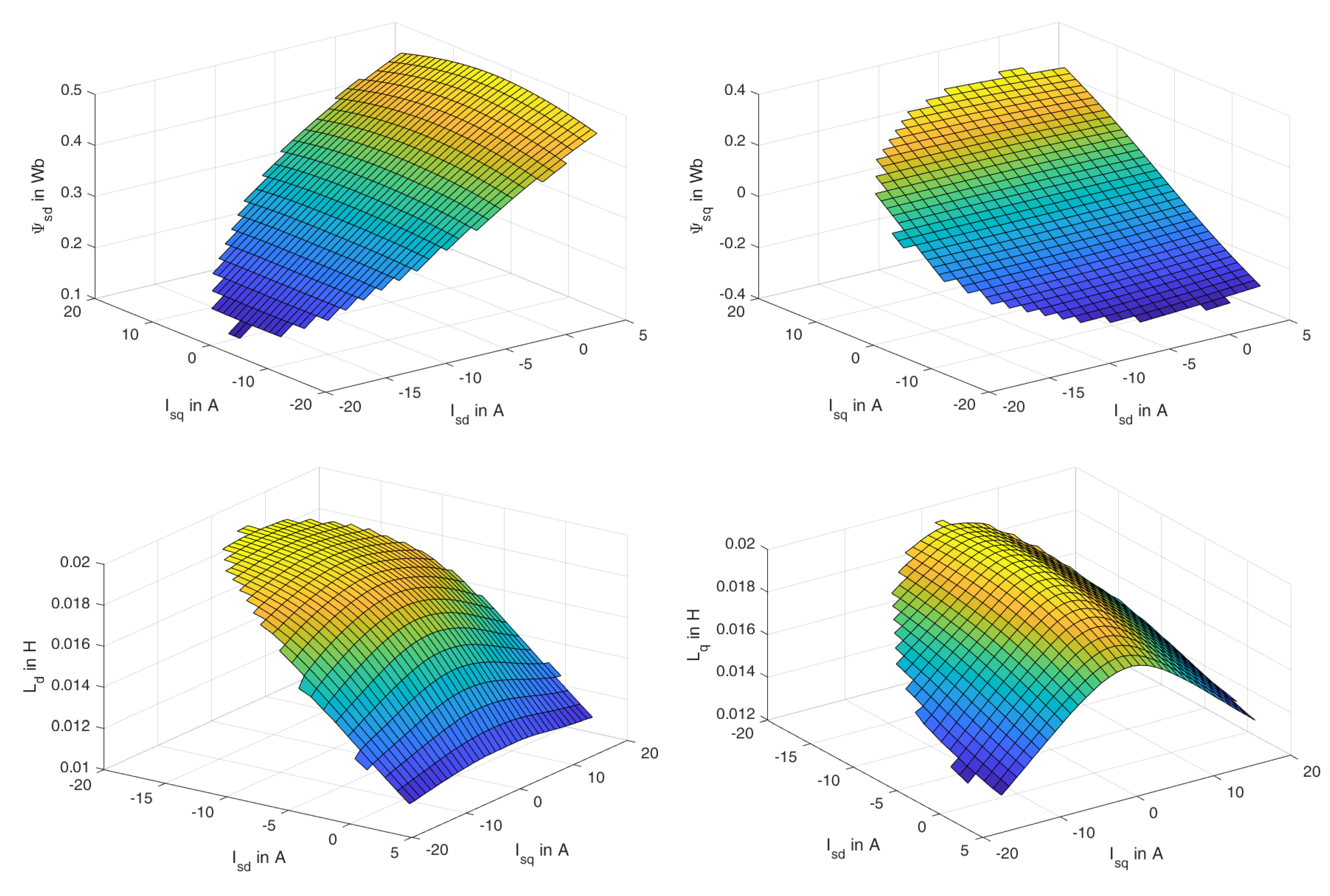
2.2.1. Flux Linkage Map (FLM)

The method is based on measuring the flux linkage map on a grid of several operating points. The motor is held at constant speed using a coupled machine (see Figure 1) and the reference currents are set from a pre-generated grid. The grid is rectangular, setpoints with a current amplitude higher than 110% of the maximum current are excluded from the measurement. In each operational point, average values of the stator currents ${(I_{sd},I_{sq})}^T$, LC filter voltages ${(U_{sd},U_{sq})}^T$, electrical speed $({\omega }_{\mathrm{el}}=n_p{\omega }_m)$, and winding temperature (${\vartheta }_s$ in °C) are computed over a measured time window of 1 s. Flux linkage maps for each axis are computed by:

$$\begin{array}{cc}\hfill {\mathsf{\Psi }}_{sd}& =\frac{1}{{\omega }_{\mathrm{el}}}(U_{sq}-R_{s\left(\mathrm{comp}\right)}{I}_{sq})\hfill \end{array}$$

(7)

$$\begin{array}{cc}\hfill {\mathsf{\Psi }}_{sq}& =\frac{1}{{\omega }_{\mathrm{el}}}(U_{sd}-R_{s\left(\mathrm{comp}\right)}{I}_{sd})\hfill \end{array}$$

(8)

$$\begin{array}{cc}\hfill R_{s\left(\mathrm{comp}\right)}& =R_{s\left(\mathrm{nom}\right)}(1+{\alpha }_{\mathrm{Cu}}({\vartheta }_s-20))\hfill \end{array}$$

(9)

where ${\mathsf{\Psi }}_{sd}$ and ${\mathsf{\Psi }}_{sq}$ denotes the averaged stator flux linkages, $R_{s\left(\mathrm{comp}\right)}$ is the temperature compensated stator resistance, $R_{s\left(\mathrm{nom}\right)}$ is the nominal value of the stator resistance, and ${\alpha }_{\mathrm{Cu}}$ is the thermal coefficient of the copper winding. The differential inductances are computed from the fluxes using:

$$\begin{array}{ccccc}\hfill L_{sd}=& \frac{\Delta {\mathsf{\Psi }}_{sd}}{\Delta I_{sd}},\hfill & \hfill L_{sq}=& \frac{\Delta {\mathsf{\Psi }}_{sq}}{\Delta I_{sq}},\hfill & \hfill L_m=\frac{\Delta {\mathsf{\Psi }}_{sd}}{\Delta I_{sq}}=\frac{\Delta {\mathsf{\Psi }}_{sq}}{\Delta I_{sd}}.\end{array}$$

(10)

The maps of flux linkages and differential self inductances $L_{sd}$ and $L_{sq}$ and mutual inductance $L_m$ of the considered machine are displayed in Figure 2. With the available maps of the flux linkages ${\mathsf{\Psi }}_{sd}$ and ${\mathsf{\Psi }}_{sq}$, the torque $m_{m,\mathrm{FLM}}$ can be computed using (4) without linearizaton.

2.2.2. Frequency Domain Identification in Standstill (OffFreq)

Rough (nominal) estimates of the $d,q$ inductances and stator resistance are obtained from analysis of the frequency characteristics of a machine at standstill. Locking the rotor (i.e., ${\omega }_{\mathrm{el}}=0$) and neglecting the mutual inductance (i.e., $L_m=0$) simplifies the model of the machine in (2) to

$$\begin{array}{cc}\hfill u_{sd}& =L_{sd}\frac{\Delta i_{sd}}{\Delta t}+R_s{i}_{sd},u_{sq}=L_{sq}\frac{\Delta i_{sq}}{\Delta t}+R_s{i}_{sq}.\hfill \end{array}$$

The response is measured for a set of frequencies (logarithmic scale is recommended, cut-off frequency $f_{\mathrm{cut}-\mathrm{off}}=\frac{R_s}{2\pi L_s}$ for nominal parameters of $R_s$ and $L_s$ should be in the middle of the frequency range). In the case of the considered IPMSM, the nominal cut-off frequencies were 15 Hz in the d axis and 10 Hz in the q axis. The responses of the system were measured at frequencies of (1, 3, 8, 24, 70, 200) Hz for both axes as illustrated in Figure 3 displaying interpolation of the measured data by the model. The responses at the tested frequencies are obtained by fast Fourier transform (FFT). Inductances and stator resistance for both axes are estimated using the Matlab System Identification Toolbox.

The main advantage of this method is its robustness. However, the values of the parameters are assumed to be constant for all operating conditions of the motor.

2.2.3. Online Frequency Domain Identification (OlFreq)

The set of methods proposed in [20] allows estimating inductances, resistance, and permanent magnet flux linkage. We consider resistance and permanent magnet flux linkage to be constant, so we use only inductances estimation.

The equivalent circuit for high frequency injected current has the same parameters as the equivalent circuit for the fundamental current component.

$$\begin{array}{cc}\hfill L_{sd}=& \frac{U_{dh}}{{\omega }_{\mathrm{inj}\left(d\right)}{I}_{dh}}sin({\theta }_{du}-{\theta }_{di})\hfill \\ \hfill L_{sq}=& \frac{U_{qh}}{{\omega }_{\mathrm{inj}\left(q\right)}{I}_{qh}}sin({\theta }_{qu}-{\theta }_{qi})\hfill \end{array}$$

(11)

Estimation is independent of the fundamental current or speed of the machine due to the current injection. The response of the high-frequency voltage excitation is extracted using discrete Fourier transform (DFT). For the convenience of DFT, ${\omega }_{inj}$ should be integer divisors of switching frequency. ${\omega }_{\mathrm{inj}\left(d\right)}$ and ${\omega }_{\mathrm{inj}\left(q\right)}$ should be sufficiently distinct to decouple the parameter identification in dq-axes. Additionally, ${\omega }_{\mathrm{inj}\left(q\right)}$ is supposed to be larger than ${\omega }_{\mathrm{inj}\left(d\right)}$, since the q-axis has greater influence on torque [20]. ${\omega }_{\mathrm{inj}}$ must avoid sixth multiples of the fundamental frequency ${\omega }_{el}$ due to the slotting effect. Both frequencies should be much higher than the nominal frequency of the machine. In the case of the considered machine, ${\omega }_{el}$ is in the range of $0÷(2\pi ·100)$ rad/s, hence the frequencies ${\omega }_{\mathrm{inj}\left(d\right)}=(2\pi ·400)$ rad/s, ${\omega }_{\mathrm{inj}\left(q\right)}=(2\pi ·500)$ rad/s, were chosen. The switching frequency was 10 kHz.

2.2.4. Recursive Least Squares (RLS)

Many variants of the RLS method have been proposed. Due to the observability problem, RLS for IPMSM model (2), additional current injection [25], or current ripple analysis [26] is recommended. The effect of the injections will be studied in the experimental section. RLS could be applied separately on each equation of model (2) linearized using (3) or as one combined estimation based on both equations [27]. We use the combined estimation for both axes. The generic estimation problem is given by

$$\begin{array}{cc}\hfill \mathit{y}=& {[{\mathit{x}}_d,{\mathit{x}}_q]}^{\top }\theta ,\hfill \\ \hfill \widehat{\theta }=& {\mathit{V}}^{-1}\mathit{W}\hfill \\ \hfill \mathit{V}=& \lambda \mathit{V}+{\mathit{x}}_{\mathit{d}}{\mathit{x}}_{\mathit{d}}^T+{\mathit{x}}_{\mathit{q}}{\mathit{x}}_{\mathit{q}}^T+\alpha \mathit{I}\hfill \\ \hfill \mathit{W}=& \lambda \mathit{W}+{\mathit{x}}_{\mathit{d}}\mathit{y}+{\mathit{x}}_{\mathit{q}}\mathit{y}\hfill \end{array}$$

(12)

and comes in two versions of the parametrization. The first one, $\mathrm{RL}{\mathrm{S}}_{\mathrm{Ls}}$, estimates only the d and q inductances, which gives the following parametrization

$$\begin{array}{cccc}\hfill {\theta }_{\mathrm{Ls}}=& \left[\begin{array}{cc}{L}_{sd}& L_{sq}\end{array}\right],\hfill & \hfill \alpha =& 0.00001,\hfill \\ \hfill {\mathit{x}}_{{\mathit{d}}_{\mathrm{Ls}}}=& \left[\begin{array}{c}\frac{\Delta i_{sd}}{\Delta t}\\ -i_{sq}{\omega }_{\mathrm{el}}\end{array}\right],\hfill & \hfill {\mathit{x}}_{{\mathit{q}}_{\mathrm{Ls}}}=& \left[\begin{array}{c}{i}_{sd}{\omega }_{\mathrm{el}}\\ \frac{\Delta i_{sq}}{\Delta t}\end{array}\right],\hfill \\ \hfill {\mathit{y}}_{\mathrm{Ls}}=& \left[\begin{array}{c}{u}_{sd}-R_s{i}_{sd}+{\omega }_{\mathrm{el}}{\psi }_{rq}\\ u_{sq}-R_s{i}_{sq}-{\omega }_{\mathrm{el}}{\psi }_{rd}\end{array}\right].\hfill \end{array}$$

(13)

The second one, $\mathrm{RL}{\mathrm{S}}_{\mathrm{Ls}{\psi }_0},$ considers ${\psi }_{0d}$ and ${\psi }_{0q}$ to depend on the operation point and has the parametrization

$$\begin{array}{cccc}\hfill {\theta }_{\mathrm{Ls}{\psi }_0}=& \left[\begin{array}{cccc}{L}_{sd}& L_{sq}& {\psi }_{0d}& {\psi }_{0q}\end{array}\right],\hfill & \hfill \alpha =& 0.00001,\hfill \\ \hfill {\mathit{x}}_{{\mathit{d}}_{\mathrm{Ls}{\psi }_0}}=& \left[\begin{array}{c}\frac{\Delta i_{sd}}{\Delta t}\\ -i_{sq}{\omega }_{\mathrm{el}}\\ 0\\ -{\omega }_{\mathrm{el}}\end{array}\right],\hfill & \hfill {\mathit{x}}_{{\mathit{q}}_{\mathrm{Ls}{\psi }_0}}=& \left[\begin{array}{c}{i}_{sd}{\omega }_{\mathrm{el}}\\ \frac{\Delta i_{sq}}{\Delta t}\\ {\omega }_{\mathrm{el}}\\ 0\end{array}\right],\hfill \\ \hfill {\mathit{y}}_{\mathrm{Ls}{\psi }_0}=& \left[\begin{array}{c}{u}_{sd}-R_s{i}_{sd}\\ u_{sq}-R_s{i}_{sq}\end{array}\right].\hfill \end{array}$$

(14)

For both parametrizations, $\alpha$ is a regularization factor to avoid numerical problems like division by zero. $\lambda$ is the forgetting factor of the RLS. In both cases, the mutual inductance was neglected $L_m=0$. Extension of both versions of RLS to estimate $L_m$ is possible, but yields worse results for the first and identical results for the second variant.

Since injection of the probing signal is known to improve the quality of estimation, both versions of the RLS method with injected current signal were also tested. For easier comparison, the same signal that is used in the OlFreq method is injected, these methods will be denoted ${\mathrm{RLS}}_{LS}^{inj}$ and ${\mathrm{RLS}}_{LS{\psi }_0}^{inj}$.

2.3. Optimal MTPC Using Torque Sensor

All methods estimating physical parameters optimize performance in the sense of MTPC. The optimal operating point in this criteria can be also found experimentally, given the measurement of the torque. Then, the optimal operating point is determined as the one with maximum ratio of the measured torque and measured current. This method, denoted as Sensor, is not practical in applications, but we will use it as a reference for the interpretation of the parametric approaches. Specifically, a perfect model of torque and current should be in agreement with the measured values, and the efficiency of such a model should approach that of the sensor method. This does not mean that this method is optimal because Joule losses form only a part of the total losses as it is demonstrated later.

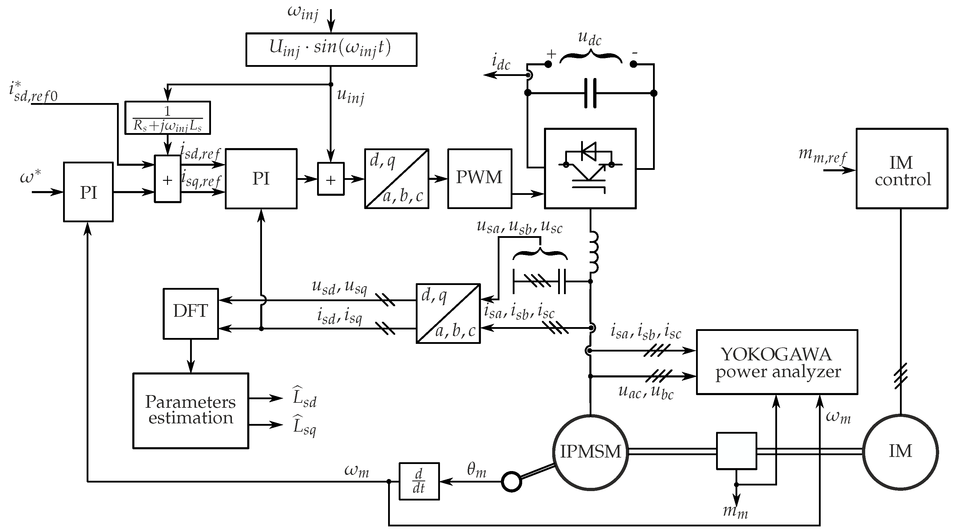
3. Laboratory Equipment

The rated power of the tested IPMSM drive is $4.5$ kW, rated voltage 400 $V_{\mathrm{RMS}}$, rated current 12.47 $A_{\mathrm{RMS}}$, rated speed 1500 rpm, and pole pair number $n_p=4$. Nominal parameters of the machine are $R_s=1.277\mathsf{\Omega },$${\psi }_{\mathrm{pm}}=0.438\mathrm{Wb},$$L_{sd}=14.0\mathrm{mH},\mathrm{and}$$L_{sq}=19.3\mathrm{mH}$. Output current from the inverter is filtered using a three-phase LC filter (see Figure 1) with inductance $L_f=0.25\mathrm{mH}$ and capacitance $C_f=100\mathsf{\mu }\mathrm{F}$. The IPMSM drive is equipped with a 12 bit absolute angular position encoder LARM ARC 405, a torque sensor Burster 8661 (output signal is filtered by a first-order lowpass RC filter with a time constant of $500\mathsf{\mu }$s), a voltage transducer LEM LV 25-P for the converter DC-link voltage measurement, and current transducers LA 55-P for measurement of the DC-link and stator phase currents. The switching frequency of the voltage-source converter, supplying the IPMSM is 10 kHz. Temperatures of the winding and the endshield of the machine are measured using a pair of Pt100 sensors with respective transducers. The coupled induction machine (IM) drive consists of a Siemens 1LE10011CB034 motor and a Siemens S120 converter.

4. Experimental Results

All experiments were performed with measured data evaluated at a steady-state operating point of the motor for predefined values of the load torque and speed. The operating point is defined by the current in the d-axis that was fixed to one of the grid points (x-axis in the plot in Figure 4). The grid of the d-axis current, −5A to +2A, was designed to cover the nominal MTPC curve with a wide margin. The tested electrical drive was loaded by constant torques (33%, 66%, and 100% of nominal torque in both directions) and driven to predefined constant speeds using a PI controller influencing the q-axis current. The resulting operating points for such constant load and speed (i.e., constant power) are then forming constant torque isolines of the machine, see Figure 4.

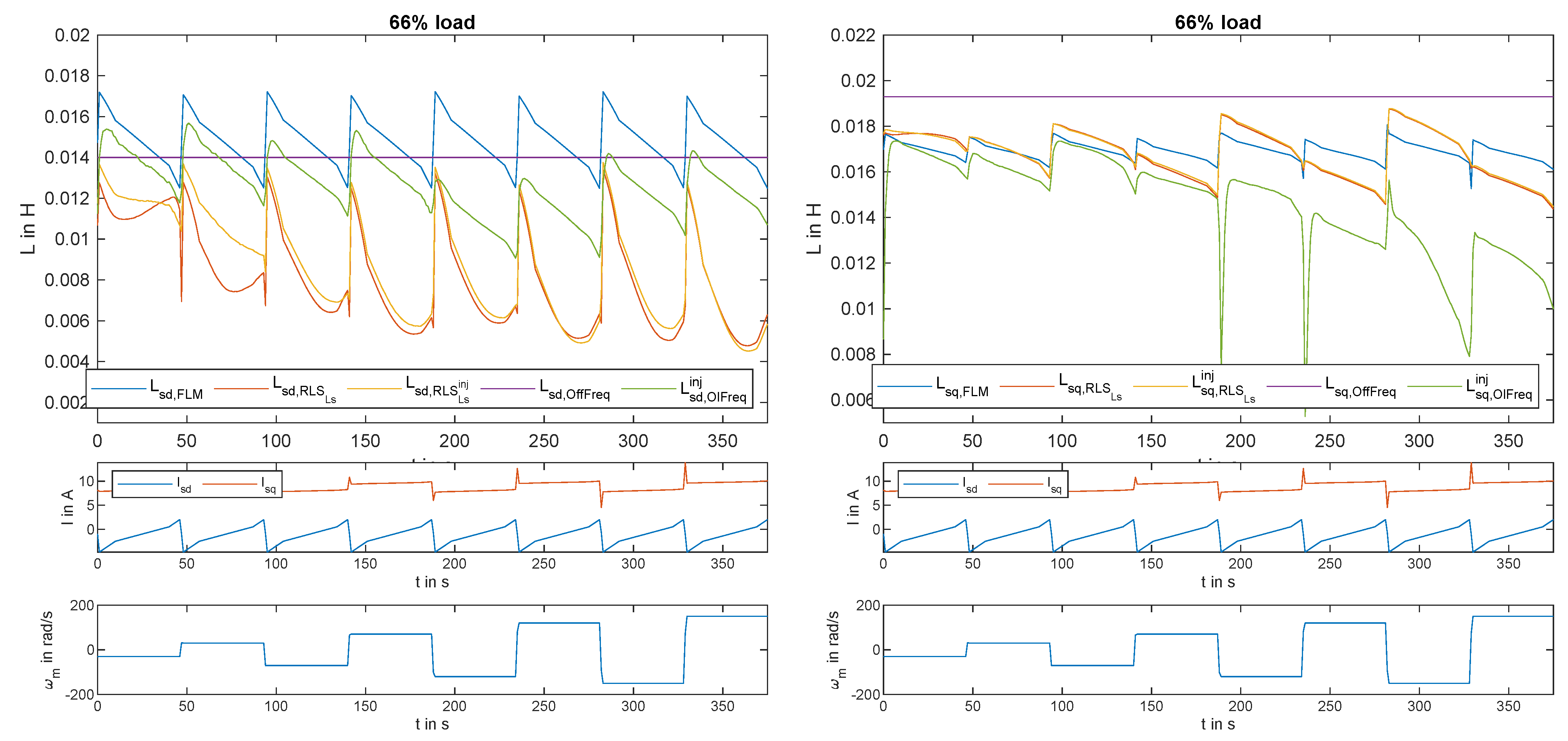
4.1. Estimated Parameters

First, we compare the estimated parameters of all model-based methods. Parameters of all methods were tuned independently to obtain the best performance. Estimates of the methods estimating only inductances (${\mathrm{RLS}}_{Ls}$ with a forgetting factor $\lambda =0.999$, frequency-characteristics methods (OffFreq, OlFreq), and FLM inductance) are shown in Figure 5. Estimated of the RLS${}_{Ls{\psi }_0}$ estimating also ${\psi }_{0d}$ and ${\psi }_{0q}$ are displayed in Figure 6. An example of the effect of each method on the torque predicted from the model using the estimated parameters is displayed in Figure 7, where the predicted torque is divided by the amplitude of the current to form the torque-per-ampere (TPC) quantity.

The provided results indicate the following:

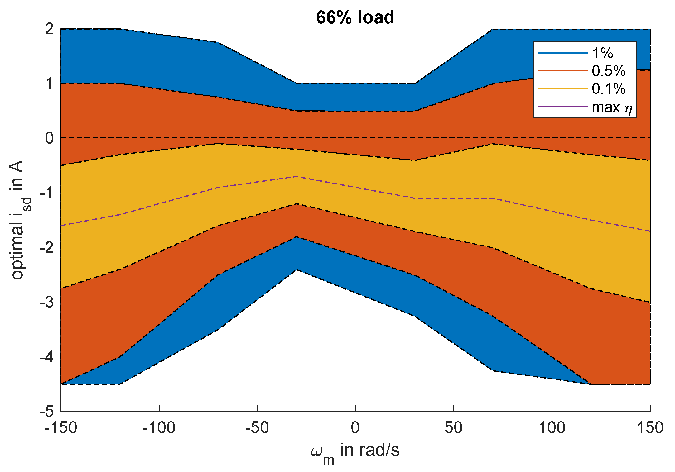
• Injections of the excitation signal significantly improve the accuracy of the RLS-based methods in all regimes except the full load conditions. This may be related to the inductance saturation or signal-to-noise ratio of the current measurements.
• For all methods with constant $\psi$, the estimated inductance is decreasing with the increasing rotation speed, and is strongly current-dependent, see Figure 5. Estimates of the inductances obtained by the RLS that jointly estimate the flux $\psi$ are stabilized at values significantly lower than nominal, the variability has been absorbed by the flux parameter, see Figure 6. This seems to be an artifact of the RLS approach, since parameter variability can be tuned in more sophisticated methods such as the extended Kalman filter.
• The peak on the $L_{sq}$ estimate obtained by the OlFreq method in Figure 5 is caused by the interference of the injected signal and multiples of the mechanical frequency during the transient.

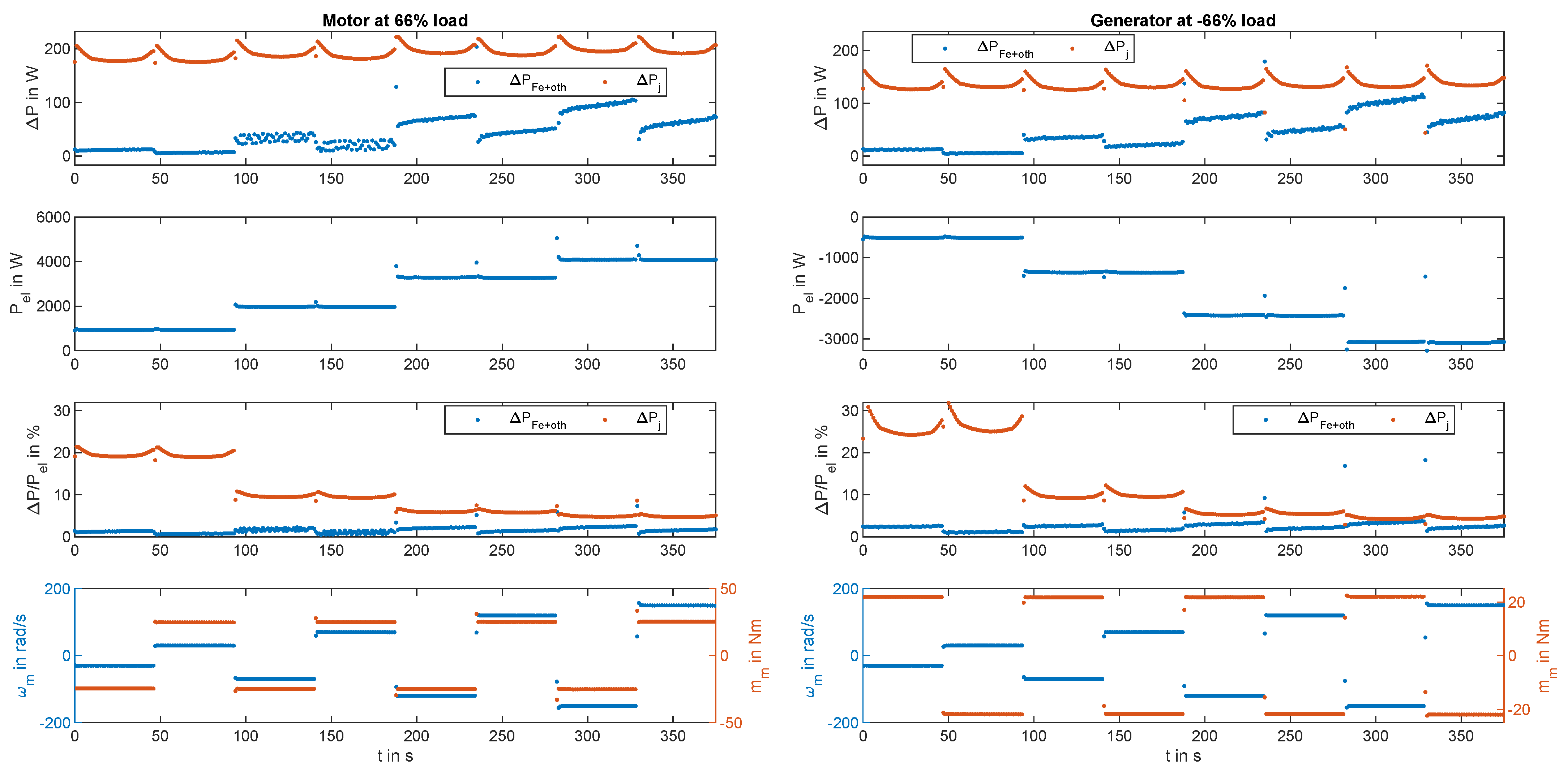
4.2. Analysis of Motor Losses

For a better understanding of the power loss decomposition, the Joule losses were computed as follows

$$\Delta P_j=3R_s{I}_s^2$$

and subtracted them from the total power loss $\Delta P_{sum}=\left|P_{el}-P_{mech}\right|$ to obtain losses in the iron and mechanical friction

$$\Delta P_{Fe+oth}=\Delta P_{sum}-\Delta P_j.$$

The decomposition of the power losses is displayed in Figure 8. An interesting conclusion is that the mechanical power losses depend on the direction of rotation, which is due to non-symmetrical Coulomb friction ([28] in Section 11.1.5). Note that Joule losses are the dominant part of the total losses for low power regimes, while mechanical and iron losses increase their importance in the high-speed regime.

4.3. Efficiency Evaluation

First, we will analyze the maximum possible efficiency of the machine that was obtained by the grid search over all possible operating points, see Figure 9. Efficiency was measured by a Yokogawa power analyzer, see Figure 1. Note that the efficiency is non-symmetric with respect to the direction of the rotation, which is caused by non-symmetry of the mechanical losses as displayed in Figure 8. Since efficiencies obtained by the tested methods are relatively close to the optimal, we will not report absolute efficiencies of the tested methods but only relative efficiency with respect to the grid-search-based maximum.

Visualization of the impact of deviation from the optimal $i_{sd}$ on the relative efficiency is displayed in Figure 10 by contours of decrease of absolute efficiency with increasing deviation from the optimal $i_{sd}$ current. Note that the most sensitive area is at low speeds.

Reference efficiency (1) was computed using measurements of the torque and voltage for all grid points of the current setpoints. The relative efficiency of each method was determined by comparing the reference efficiency at the optimal (grid-searched) setpoint $i_{sd}^{*}$ with reference efficiency evaluated at the setpoint provided by the tested method, $i_{sd,\mathrm{method}}$, i.e., ${\eta }_{\mathrm{rel}}=\frac{{\eta }_{\mathrm{ref}}\left({\mathit{i}}_s\left(i_{sd,\mathrm{method}}\right)\right)}{{\eta }_{\mathrm{ref}}\left({\mathit{i}}_s\left(i_{sd}^{*}\right)\right)}$ as visualized in Figure 11.

The value of the d-component of the stator current that was selected by the MTPC strategy evaluated for each method and $i_{sd}$ for the maximum reference efficiency is shown for three different load torque levels in both directions in Figure 12. The average of the relative efficiency of the motor for various methods at various loads is compared in Figure 13. Note that the relative efficiency of many methods is decreasing, especially at high load. The most significant drop is for the online frequency-domain identification (OlFreq), but it is also visible on both RLS variants and to some extend FLM. The offline frequency domain identification achieves the best performance.

4.4. Discussion

The results provided in the previous subsection indicate that none of the tested online identification methods were able to provide results that would reliably outperform control with carefully estimated constant parameters. However, it revealed interesting points that need to be addressed by future research which are now shortly discussed:

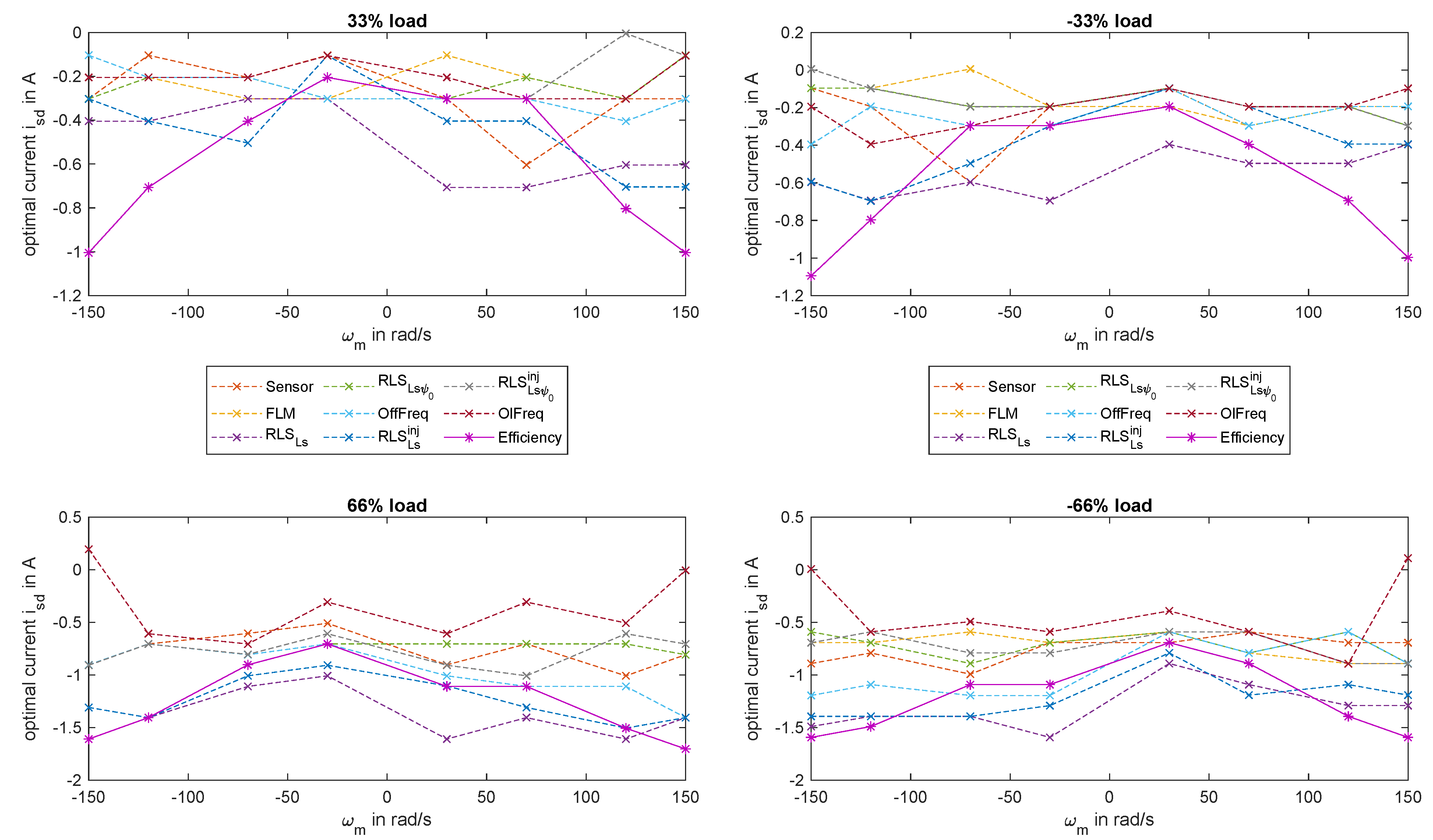
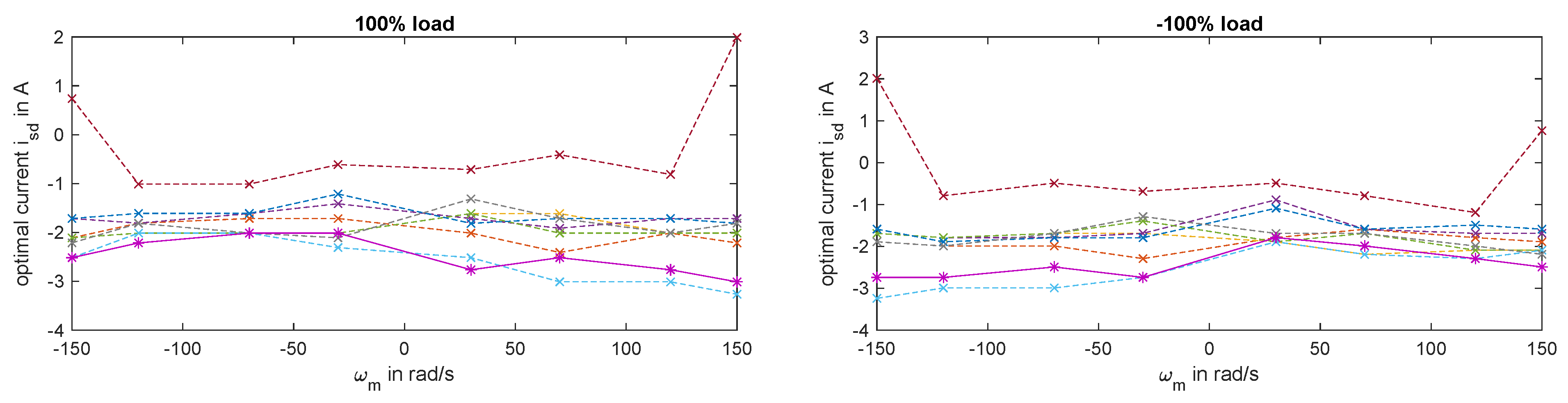
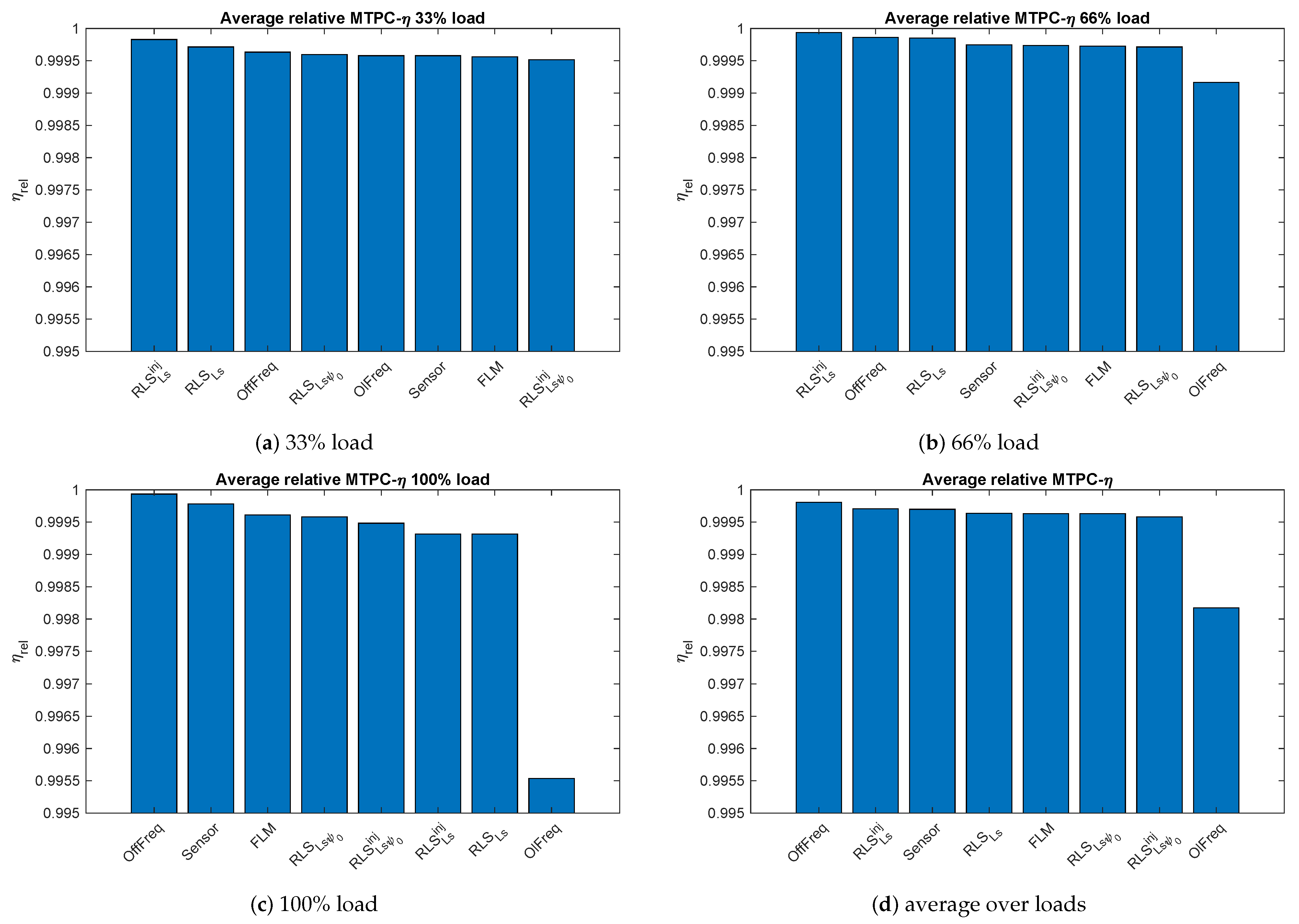
• All parametric methods optimize the MPTC and in ideal condition should approach the results of the Sensor method which measures the optimal MPTC. However, it is not the most efficient method when other losses are taken into account. Thus bias in the estimated parameters method may actually improve the overall efficiency of the method if the bias is systematic towards the overall efficiency. This seems to be the case for the OffFreq method, which always performs better than Sensor and the RLS version at low loads. This clearly suggests that MTPC is not the optimal criteria and should be replaced by maximum torque per losses (MPTL) which also minimizes iron losses in the machine (for details see [10,29]).
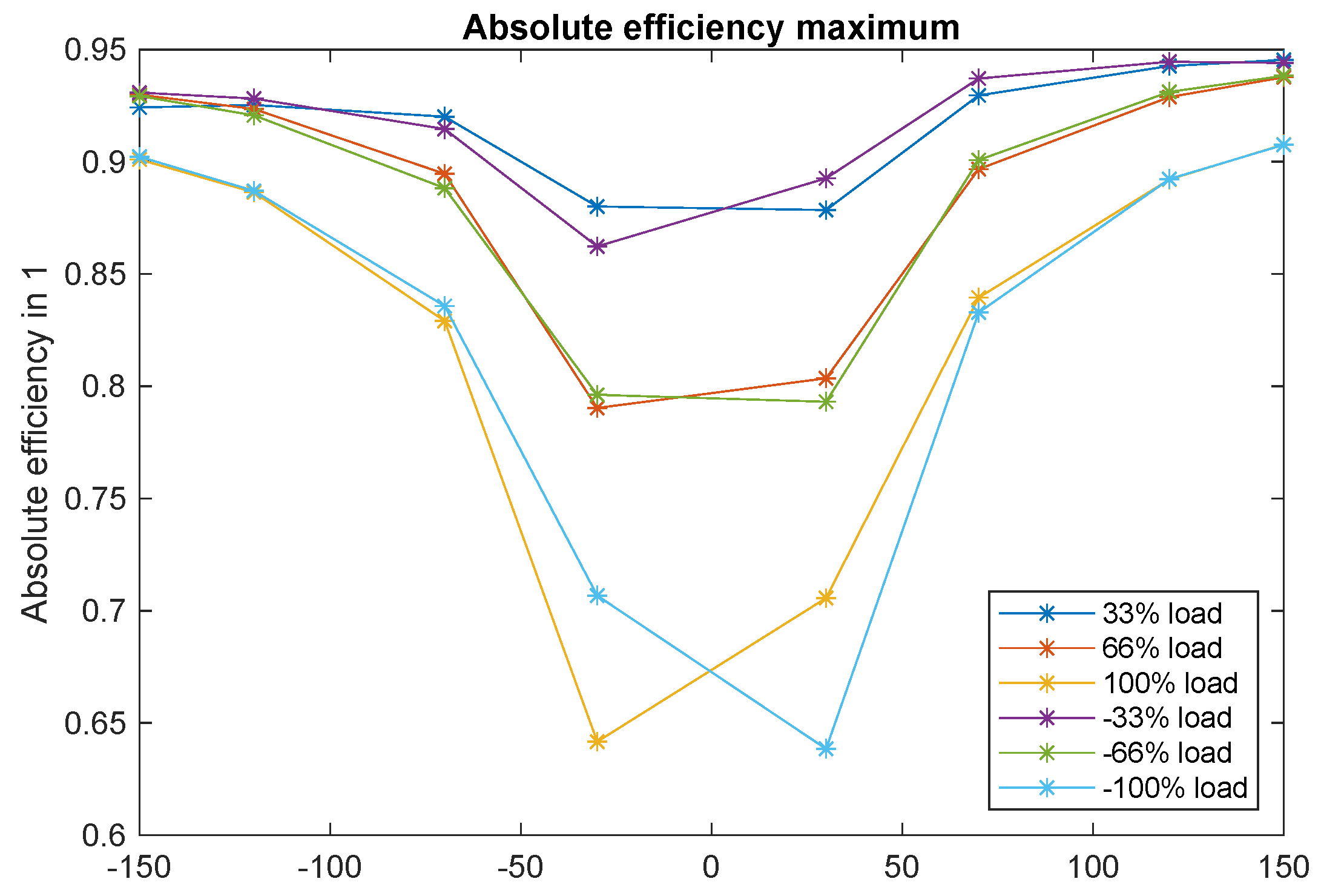
• The best overall efficiency was obtained for parameters obtained from offline identification by the frequency analysis, see Figure 13. This is due to its consistency, being one of the top three methods at all loads. It is clearly the best at 100% load condition. For lower loads, the RLS${}_{LS}^{inj}$ method achieves marginally better results. This may be surprising, since OffFreq uses fixed parameters without any adaptation to operating conditions. This suggests that consistency of the method across operating regimes is more important than its accuracy under come conditions. This can be demonstrated by the OlFreq methods that perform well under 33% loads, but quickly deteriorates for higher loads.
• The findings of [23] that RLS is capable to improve drive efficiency are confirmed only for profiles with a low percentage of the full load operation. If the profile contains more full load conditions, the outcome may be quite the opposite and the RLS will yield worse efficiency than that with constant parameters. However, such conditions are unlikely in many applications such as electro-mobility and the use of RLS for parameter estimation can be recommended.
• The relative efficiency of the methods based on RLS slightly improves with the injection of the excitation signal. However, a decrease in performance was also observed for the ${\mathrm{RLS}}_{Ls{\psi }_0}$ method.

5. Conclusions

We compared the behavior of various methods for optimal feed-forward torque control to assess the suitability of feed-forward control with online parameter estimation methods for operating IPMSM with maximum efficiency. The frequency identification method, method based on torque sensor measurement, flux linkage map method, and RLS methods obtained comparable results. While methods based on RLS achieved good performance in low load conditions, they proved to be unreliable in full load conditions. The least reliable method was the online frequency domain estimation method. None of the online parameter identification methods were able to obtain reliable performance under full load conditions, indicating the need for the development of new methods.

Moreover, the experiments also demonstrated that the feed-forward controller based on the MTPC may significantly differ from the optimum efficiency operating point. This may be improved by optimizing the criteria considering other kinds of losses, however, this increases the number of parameters which imposes another challenge on parameter identification and most importantly its reliability. Clearly, more research in this direction is required.

References

1. Brousek, J.; Krcmar, L.; Rydlo, P. Efficiency Measuring of Electric Drive with Traction Synchronous Motor with Permanent Magnets. In Proceedings of the 2021 IEEE International Workshop of Electronics, Control, Measurement, Signals and their application to Mechatronics (ECMSM), Liberec, Czech Republic, 21–22 June 2021; pp. 1–5. [Google Scholar] [CrossRef]
2. Sivkov, O.; Novak, J. Flux Weakening Control of Permanent Magnet Synchronous Motor with Losses Reduction. In Proceedings of the 2021 XVIII International Scientific Technical Conference Alternating Current Electric Drives (ACED), Ekaterinburg, Russia, 24–27 May 2021; pp. 1–6. [Google Scholar] [CrossRef]
3. Stipetic, S.; Goss, J.; Zarko, D.; Popescu, M. Calculation of Efficiency Maps Using a Scalable Saturated Model of Synchronous Permanent Magnet Machines. IEEE Trans. Ind. Appl. 2018, 54, 4257–4267. [Google Scholar] [CrossRef]
4. Rassolkin, A.; Heidari, H.; Kallaste, A.; Vaimann, T.; Acedo, J.P.; Romero-Cadaval, E. Efficiency Map Comparison of Induction and Synchronous Reluctance Motors. In Proceedings of the 2019 26th International Workshop on Electric Drives: Improvement in Efficiency of Electric Drives (IWED), Moscow, Russia, 30 January–2 February 2019; pp. 1–4. [Google Scholar] [CrossRef]
5. Ferrari, S.; Ragazzo, P.; Dilevrano, G.; Pellegrino, G. Flux-Map Based FEA Evaluation of Synchronous Machine Efficiency Maps. In Proceedings of the 2021 IEEE Workshop on Electrical Machines Design, Control and Diagnosis (WEMDCD), Modena, Italy, 8–9 April 2021; pp. 76–81. [Google Scholar] [CrossRef]
6. Jiang, W.; Feng, S.; Zhang, Z.; Zhang, J.; Zhang, Z. Study of Efficiency Characteristics of Interior Permanent Magnet Synchronous Motors. IEEE Trans. Magn. 2018, 54, 1–5. [Google Scholar] [CrossRef]
7. Golzar, M.; Van Khang, H.; Hubert Choux, M.M.; Midtbo Versland, A.M. Experimental Investigation of Efficiency Map for an Inverter-Fed Surface-Mount Permanent Magnet Synchronous Motor. In Proceedings of the 2019 8th International Conference on Renewable Energy Research and Applications (ICRERA), Brasov, Romania, 3–6 November 2019; pp. 551–556. [Google Scholar] [CrossRef]
8. Eldeeb, H.; Hackl, C.M.; Horlbeck, L.; Kullick, J. A unified theory for optimal feedforward torque control of anisotropic synchronous machines. Int. J. Control 2018, 91, 2273–2302. [Google Scholar] [CrossRef]
9. Chen, Z.; Li, W.; Shu, X.; Shen, J.; Zhang, Y.; Shen, S. Operation Efficiency Optimization for Permanent Magnet Synchronous Motor Based on Improved Particle Swarm Optimization. IEEE Access 2021, 9, 777–788. [Google Scholar] [CrossRef]
10. Hackl, C.; Kullick, J.; Monzen, N. Generic loss minimization for nonlinear synchronous machines by analytical computation of optimal reference currents considering copper and iron losses. In Proceedings of the 2021 22nd IEEE International Conference on Industrial Technology (ICIT), Valencia, Spain, 10–12 March 2021; Volume 1, pp. 1348–1355. [Google Scholar] [CrossRef]
11. Glac, A.; Šmídl, V.; Peroutka, Z. Optimal Feedforward Torque Control of Synchronous Machines with Time-Varying Parameters. In Proceedings of the IECON 2018—44th Annual Conference of the IEEE Industrial Electronics Society, Washington, DC, USA, 21–23 October 2018; pp. 613–618. [Google Scholar] [CrossRef]
12. Glac, A.; Šmídl, V.; Peroutka, Z.; Hackl, C.M. Comparison of IPMSM Parameter Estimation Methods for Motor Efficiency. In Proceedings of the IECON 2020 The 46th Annual Conference of the IEEE Industrial Electronics Society, Singapore, 18–21 October 2020; pp. 895–900. [Google Scholar] [CrossRef]
13. Eldeeb, H.M.; Abdel-Khalik, A.S.; Hackl, C.M. Dynamic Modeling of Dual Three-Phase IPMSM Drives With Different Neutral Configurations. IEEE Trans. Ind. Electron. 2019, 66, 141–151. [Google Scholar] [CrossRef]
14. Liu, K.; Feng, J.; Guo, S.; Xiao, L.; Zhu, Z. Identification of Flux Linkage Map of Permanent Magnet Synchronous Machines Under Uncertain Circuit Resistance and Inverter Nonlinearity. IEEE Trans. Ind. Inform. 2018, 14, 556–568. [Google Scholar] [CrossRef]
15. Brosch, A.; Hanke, S.; Wallscheid, O.; Böcker, J. Data-Driven Recursive Least Squares Estimation for Model Predictive Current Control of Permanent Magnet Synchronous Motors. IEEE Trans. Power Electron. 2021, 36, 2179–2190. [Google Scholar] [CrossRef]
16. Rafaq, M.S.; Jung, J.W. A Comprehensive Review of State-of-the-Art Parameter Estimation Techniques for Permanent Magnet Synchronous Motors in Wide Speed Range. IEEE Trans. Ind. Inform. 2020, 16, 4747–4758. [Google Scholar] [CrossRef]
17. Li, X.; Kennel, R. Comparison of state-of-the-art estimators for electrical parameter identification of PMSM. In Proceedings of the 2019 IEEE International Symposium on Predictive Control of Electrical Drives and Power Electronics (PRECEDE), Quanzhou, China, 31 May–2 June 2019; pp. 1–6. [Google Scholar] [CrossRef]
18. Li, S.; Sarlioglu, B.; Jurkovic, S.; Patel, N.R.; Savagian, P. Comparative Analysis of Torque Compensation Control Algorithms of Interior Permanent Magnet Machines for Automotive Applications Considering the Effects of Temperature Variation. IEEE Trans. Transp. Electrif. 2017, 3, 668–681. [Google Scholar] [CrossRef]
19. Zhu, Z.Q.; Liang, D.; Liu, K. Online Parameter Estimation for Permanent Magnet Synchronous Machines: An Overview. IEEE Access 2021, 9, 59059–59084. [Google Scholar] [CrossRef]
20. Wang, Q.; Wang, G.; Zhao, N.; Zhang, G.; Cui, Q.; Xu, D. An Impedance Model-Based Multiparameter Identification Method of PMSM for Both Offline and Online Conditions. IEEE Trans. Power Electron. 2021, 36, 727–738. [Google Scholar] [CrossRef]
21. Kallio, S.; Karttunen, J.; Peltoniemi, P.; Silventoinen, P.; Pyrhönen, O. Online Estimation of Double-Star IPM Machine Parameters Using RLS Algorithm. IEEE Trans. Ind. Electron. 2014, 61, 4519–4530. [Google Scholar] [CrossRef]
22. Cao, M.; Migita, H. A High Efficiency Control of IPMSM with Online Parameter Estimation. In Proceedings of the 2018 21st International Conference on Electrical Machines and Systems (ICEMS), Jeju, Korea, 7–10 October 2018; pp. 1421–1424. [Google Scholar] [CrossRef]
23. Nguyen, Q.K.; Petrich, M.; Roth-Stielow, J. Implementation of the MTPA and MTPV control with online parameter identification for a high speed IPMSM used as traction drive. In Proceedings of the 2014 International Power Electronics Conference (IPEC-Hiroshima 2014—ECCE ASIA), Hiroshima, Japan, 18–21 May 2014; pp. 318–323. [Google Scholar] [CrossRef]
24. Noguchi, T.; Kumakiri, Y. On-line parameter identification of IPM motor using instantaneous reactive power for robust maximum torque per ampere control. In Proceedings of the 2015 IEEE International Conference on Industrial Technology (ICIT), Seville, Spain, 17–19 March 2015. [Google Scholar] [CrossRef]
25. Nalakath, S.; Preindl, M.; Emadi, A. Online multi-parameter estimation of interior permanent magnet motor drives with finite control set model predictive control. IET Electr. Power Appl. 2017, 11, 944–951. [Google Scholar] [CrossRef] [Green Version]
26. Choi, K.; Kim, Y.; Kim, K.; Kim, S. Using the Stator Current Ripple Model for Real-Time Estimation of Full Parameters of a Permanent Magnet Synchronous Motor. IEEE Access 2019, 7, 33369–33379. [Google Scholar] [CrossRef]
27. Xu, Y.; Yang, K.; Liu, A.; Wang, X.; Jiang, F. Online Parameter Identification Based on MTPA Operation for IPMSM. In Proceedings of the 2019 22nd International Conference on Electrical Machines and Systems (ICEMS), Harbin, China, 11–14 August 2019; pp. 1–4. [Google Scholar] [CrossRef]
28. Hackl, C.M. Speed and Position Control of Industrial Servo-Systems. In Non-Identifier Based Adaptive Control in Mechatronics: Theory and Application; Springer International Publishing: Cham, Switzerland, 2017; pp. 321–433. [Google Scholar] [CrossRef]
29. Hackl, C.; Kullick, J.; Monzen, N.; Böcker, J.; Griepentrog, G. Optimale betriebsführung für nichtlineare synchronmaschinen. In Elektrische Antriebe–Regelung von Antriebssystemen; Böcker, J., Griepentrog, G., Eds.; Springer: Berlin/Heidelberg, Germany, 2020. [Google Scholar]
Figure 1. Control block diagram of the experimental rig including injection of high frequency signal.
Sustainability 13 09299 g001
Figure 2. Identified maps for the FLM method. (Top row): Flux linkage maps for d (left) and q (right) axis. (Middle row): Differential self inductances maps for d (left) and q (right) axis. (Bottom row): Differential mutual inductances maps for d (left) and q (right) axis.
Sustainability 13 09299 g002aSustainability 13 09299 g002b
Figure 3. Frequency domain identification experiment—measured points of the frequency response and analytically computed response for the identified parameters.
Sustainability 13 09299 g003
Figure 4. The grid of operating points on which is evaluated performance of all methods (fixed d-grid, q-axis current is set by a PI controller of the speed). The grid is constructed around the MTPC (MTPA) curve computed from parameters identified at the standstill.
Sustainability 13 09299 g004
Figure 5. Estimated inductance L s d (left) and L s q (right) using five methods: (i) flux linkage map, L * , F L M , (ii) RLS Ls , (iii) RLS Ls i n j , (iv) frequency domain identification at standstill L * , O f f F r e q , and (v) online frequency domain identification, L * , O l F r e q . Profile of the current and torque under which the parameters were identified is displayed in the two bottom subplots of the figure, respectively.
Sustainability 13 09299 g005
Figure 6. Estimated inductances L s d and L s q and magnetic fluxes ψ 0 d and ψ 0 q using RLS Ls ψ 0 and RLS Ls ψ 0 i n j . Profile of the current and torque under which the parameters were identified is displayed in the two bottom subplots of the figure, respectively.
Sustainability 13 09299 g006
Figure 7. Example of calculation of the operating point using MTPC for all parametric models and the Sensor method at motor speed 120 rad/s and 66% of the load.
Sustainability 13 09299 g007
Figure 8. Analysis of the motor losses at 66% load at motor (left) and generator (right) regime. (Top): Joule losses Δ P j and other losses Δ P Fe + oth . (Top-middle): electric power. (Bottom-middle): ratio of losses with respect to electric power. (Bottom): operating speed and torque of the machine.
Sustainability 13 09299 g008
Figure 9. Absolute efficiency of the motor evaluated at different speed and loads.
Sustainability 13 09299 g009
Figure 10. Map of relative efficiency drop with increasing distance from the optimal i s d operating point.
Sustainability 13 09299 g010
Figure 11. Visualization of evaluation of the relative efficiency. Reference efficiency values (crosses) are interpolated using quadratic polynomial. Operation point i s d , method for each method is obtained, e.g., by maximizing TPC, and reference efficiency in the i s d , method computed (indicated by arrow). Relative efficiency is the ratio of the maximum achievable efficiency (upper dotted line) and the efficiency of TPC of the evaluated method (lower dotted line).
Sustainability 13 09299 g011
Figure 12. Comparison of the selected d-axis component of stator current for all tested methods at ±33% load (top), ±66% load (middle), and ±100% load (bottom).
Sustainability 13 09299 g012aSustainability 13 09299 g012b
Figure 13. Relative motor efficiency for the tested methods in descending order for (a) 33% of the nominal load, (b) 66% of the nominal load, (c) 100% of the nominal load, and (d) average of all load conditions. The efficiencies are averaged over all speed conditions.
Sustainability 13 09299 g013
Publisher’s Note: MDPI stays neutral with regard to jurisdictional claims in published maps and institutional affiliations.