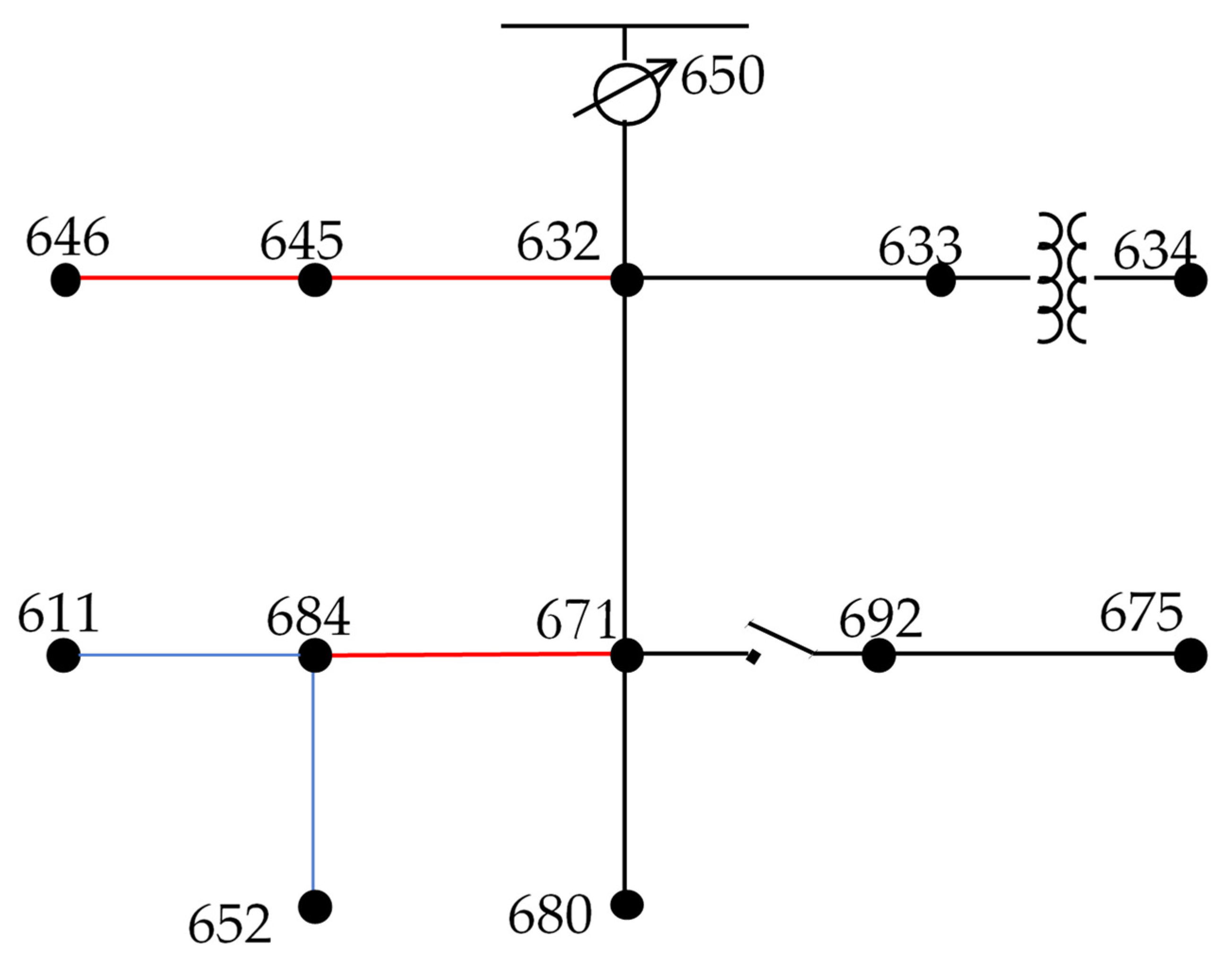
Article

Simulation Studies to Quantify the Impact of Demand Side Management on Environmental Footprint

by
Sulaiman A. Almohaimeed
1,*,
Siddharth Suryanarayanan
2 and
Peter O’Neill
3
1
Department of Electrical Engineering, College of Engineering, Qassim University, Unaizah 56452, Saudi Arabia
2
Department of Electrical Engineering & Computer Science, South Dakota State University, Brookings, SD 57007, USA
3
Retired Electrical Engineer, Fort Collins, CO 80523, USA
*
Author to whom correspondence should be addressed.
Sustainability 2021, 13(17), 9504; https://doi.org/10.3390/su13179504
Submission received: 22 June 2021 / Revised: 7 August 2021 / Accepted: 20 August 2021 / Published: 24 August 2021

Abstract

:
The increased use of energy leads to increased energy-related emissions. Demand side management (DSM) is a potential means of mitigating these emissions from electric utility generating units. DSM can significantly reduce emissions and provide economic and reliability benefits. This work presents some DSM techniques, such as load shifting, energy conservation, and valley filling. Furthermore, this work explains the most common DSM programs. To quantify the effect of DSM in diminishing carbon footprint, this paper performs power flow analysis on a yearly load profile corresponding to Fort Collins, Colorado, U.S. This work used the IEEE 13-node test system to simulate several scenarios from the multi-criteria decision-making (MCDM) alternatives, both individually and integrated. For the base case, emissions decrease by 16% from the 2005 level. The “energy conservation” option achieved a 20% reduction in emissions, integrating both alternatives increased the emissions mitigation up to 22%. Simulation of the residential sector shows the “communication and intelligence” option reduces emissions about 14% from the 2005 level. A scenario that combines “electric stationary storage” with “communication and intelligence” diminishes the emissions by more than 15%. The last scenario examined all MCDM alternatives combined into one option, resulting in a 20% emissions reduction. We also conducted a cost benefit analysis (CBA) to investigate economic, technical, and environmental costs and benefits associated with each alternative. The economic evaluation shows that “electric stationary storage” is the best option since it charges during lower electricity prices and discharges during peaking demand. The economic analysis presents a trade-off chart, so the decision maker can select the alternative based on their preference.

1. Introduction

The increased use of energy leads to increased energy-related emissions. It is important to control the greenhouse gas (GHG) portion of these emissions from electric generating units. The previous work presented in [1] discussed several governmental plans to mitigate the impact of GHG. Reference [1] also investigated using MCDM algorithms to pare down the numerous options for demand side management (DSM) by establishing a problem framework corresponding to the Climate Action Plan (CAP) goals of Fort Collins, Colorado, U.S. The findings showed that “communication and intelligence” has the highest impact in meeting the goal followed by “stationary electric storage” and “energy conservation”.
This manuscript aims to prioritize the MCDM alternatives based on their environmental impact. This work evaluates the environmental and economic aspects of the MCDM alternatives to find an optimal combination among the DSM options. In that regard, the paper quantifies the impact of DSM in reducing the environmental footprints using the IEEE 13-node test feeder through the Open Distribution System Simulator® (OpenDSS®) to perform power flow analysis on the yearly load profile of Fort Collins, Colorado, U.S. The analysis includes the simulation for several scenarios from the MCDM alternatives. It also employs an economic assessment to ensure that the proposed alternatives are economically accepted.
IEEE 13-node is a test feeder that was developed to perform distribution system analysis [2]. We use this test feeder to simulate and test the performance of MCDM alternatives in achieving reductions in emissions. Cost-benefit analysis (CBA) is an economic framework to compare several options and select the one that provides the maximum benefits. CBA is an analytical tool used to help decision makers to evaluate the available options. There are two major types of CBA: ex-ante CBA, where the analysis is constructed while the project is under consideration or before its implementation, and ex-post CBA that is conducted at the end of the project [3]. CBA is used to study the economic viability of several applications such as the Smart Grid, DR, energy storage, and RES [4,5,6,7,8].
OpenDSS® is an open-source environment developed by EPRI [9] to perform power flow studies in electric distribution systems. It has several capabilities such as general distribution planning and analysis, integration of DER, and load and storage assets.
We present methods from the literature for calculating GHG emissions from a distribution system modeled on the IEEE 13-node test feeder. This work also analyzes hourly load data from 2017 corresponding to Fort Collins [10]. The analysis includes simulating the base case load profile and then considering the MCDM options as a solution for emissions reduction. Such analysis includes performing radial power flow studies on the IEEE 13-node test feeder in normal steady-state operation. Then, the obtained results are converted into environmental metrics to calculate the GHG contribution from specific assets [10]. Further, this work implements a CBA on the MCDM alternatives.
The rest of this paper is organized as follows: Section 2 provides a brief overview of the IEEE 13-node test system, the modeling and simulation of the distribution system is discussed through a case study of Fort Collins in Section 3, Section 4 performs an economic evaluation of the prioritized MCDM alternatives, and Section 5 concludes and discusses the future path.

2. IEEE Modified Test System

The IEEE 13-node system is a small standard circuit model that was designed to test some features of the distribution system and to benchmark algorithms in solving unbalanced three-phase radial systems [2,11,12]. This distribution system is supplied at one end, as illustrated in Figure 1. The system is characterized by being short and highly loaded and interconnected with the following characteristics: (a) 10 overhead and underground lines, (b) 1 generation unit, (c) 1 voltage regulator unit, (d) 1 ΔY 115/4.16 kV transformer, (e) 1 YY 4.16/0.480 kV (in-line transformer), (f) 2 shunt capacitor banks, and (g) unbalanced spot and distributed loads.
This test feeder includes data for lines, transformers, capacitors, spot loads, and distributed loads. The next section explains the findings after simulating the base case on a distribution system emulating the one in Fort Collins. We also present some strategies to test the ability of the MCDM solutions in achieving emissions reductions.

3. Modeling and Simulation of the Distribution Systems

The need to shape the load profile by controlling demand became apparent in the 1970s [13]. Electric load profiles change daily, seasonally, and annually. Therefore, this simulation considers the yearly load profile from which we can obtain the output of the generators to meet the demand and, in turn, estimate the GHG emissions. To determine the environmental impact, the load profile corresponding to Fort Collins is translated and mapped on the IEEE 13-node system through the OpenDSS® simulation tool. The IEEE 13-node test feeder is designed to evaluate and benchmark algorithms, and this test system provides simple ways to modify the test feeders to include DERs. Thus, it is used to adapt the load of the Fort Collins distribution grid on the small circuit test system. The load curve in 2017 has a peak of 660 MW. This demand curve is scaled down to match the peak of the IEEE 13-node test system, i.e., 3.577 MW. To establish a strategy for GHG reduction, this section simulates the load profile and generation mix for the base case. After that, the analysis considers different scenarios from the MCDM options to reduce the GHG emissions compared to the base case. The analysis also combines several scenarios from among the MCDM alternatives to simulate their emissions reduction and to investigate the effectiveness of each alternative in achieving the goal. In that regard, the work studies the most preferred alternatives from the MCDM ranking list from [1], i.e., communication and intelligence, stationary storage, and energy conservation.

3.1. Base Case

To obtain the load profile and generation mix for the year 2017, using OpenDSS® with the COM interface, the actual load curve is mapped on the test system. Figure 2 illustrates the demand curve and generation mix for the base case on the IEEE 13-node test feeder using Fort Collins load data. This figure indicates that the annual peak demand occurred on 19 July 2017, at 3 pm. After analyzing the supply and demand curves, environmental assessment calculates the emissions generated from the conventional generating units for meeting the demand. Four generators use fossil fuels (and consequently emit CO2) in the system: (a) coal 1, (b) coal 2, (c) coal 3, and (d) natural gas [14].
The base case results in Figure 3 show that the emissions from the electricity sector is 13,692 tons of CO2 per year. A GHG equivalence calculator equates this to the emissions produced by burning more than 7484.29 tons of coal per year and the captured emissions from about 16,115 acres of the U.S. forests in one year [15]. As the city’s energy environmental indicator shows a 16% emissions reduction in 2017 from 2005 level due to the utilization of more renewable generation, the simulation follows with the same reduction in emissions from 2005 level of 16.26% for the same year [16].

3.2. ESS

Storage is one of the top priorities of MCDM technologies [1]. ESS can be used during peak hours to shave the load using the energy stored in ESS during off-peak periods [17]. This, in turn, minimizes the need for powering on generators that emit high volumes of CO2 during times of high demand. Platte River Power Authority (PRPA), an electric utility that generates and delivers electricity in Fort Collins, proposes using a Li-ion battery since it is the second most used technology (after Pb-acid) in the stationary storage market. Furthermore, the Li-ion technology can operate over more and deeper cycles than a lead acid battery, resulting in a lower cost per cycle. PRPA proposes batteries that can supply a peak power or 50 MW for four hours, totaling 200 MWh of energy storage.
This simulation scales down the storage parameters to fit the test system. Therefore, the ESS provides about 271 kW for the duration of four hours (i.e., 1084 kWh) to shave the peak load. After looking at the 2017 load curve, it is noteworthy that the peak hourly load usually exceeds the average hourly load by 20%. Thus, the simulation is designed to enable the ESS to shave 10% of the peak load when the load at the specified hour exceeds the average load by 20%. Coincident peak refers to the highest user demand that occurs one hour a month when the system demand is at its highest [18]. During the coincident peak, a storage system can provide aggressive reductions in peaking load, say, up to 15%. The storage system remains inactive when the load is lower than 120% of the average load. The system charges the energy storage during off-peak hours when the load is at its lowest.
i f   [ L ( t ) > a v g .   l o a d 1.2   t h e n   L ( t ) N e w = L ( t ) 0.9     L ( t ) > a v g .   l o a d 1.2   a t   c o i n c i d e n t   p e a k   t h e n   L ( t ) N e w = L ( t ) 0.85 L ( t ) a v g .   l o a d 1.2   t h e n   L ( t ) N e w = L ( t )
Figure 4 shows the load and generation mix from the test system for 2017, while Figure 5 represents a simulation of the load profile on 5 September 2019. The results show that ESS, operated according to the charge–discharge technique described above, mitigates the total emissions from the 2005 level by 18.13%, equivalent to 13,385 tons of CO2 per year. Figure 6 explains the emissions reduction per source over a year after integrating ESS. This mitigation comes from diminishing the emissions from the coal 1 power plant.

3.3. Energy Conservation

This alternative means reducing the demand and, thus, the energy needed to supply it. Energy conservation can be implemented either by deploying more energy-efficient loads or educating users to change their usage behavior to reduce the work requested of the system. In that regard, this scenario uses the ideal case for the simulation based on a 5% reduction of the entire load. Therefore, a one-year simulation is implemented after reducing the demand by 5% at all time steps. The red curve in Figure 7 illustrates such a reduction in the total demand curve for 2017. This energy saving successfully minimized the total emissions by more than 20% compared to the 2005 level. The amount of emissions generated from the test system after reducing the energy demand is equal to 13,016 tons of CO2 per year, compared to 16,350 tons of CO2 in 2005. Figure 8 demonstrates this notable mitigation in emissions. The major reduction comes from coal 1 power plant where the emissions are reduced by about 458 CO2 tons.

3.4. ESS with Energy Conservation

This scenario studies the load behavior and emissions amount after combining the two options: ESS and energy conservation. The aim of considering such a scenario is to investigate the potential of achieving greater reductions in emissions than deploying just one option. This scenario follows the same simulation strategies for ESS and conservation programs that are explained in Section 3.2 and Section 3.3. Figure 9 illustrates that such a combination affects the total energy demand. This scenario can achieve a 22% reduction in emissions, which is more than the city’s goal of reaching a 20% emissions reduction by 2020. As stated, the base case generates 16,350 CO2 tons of emissions while this option can minimize it to 12,725 CO2 tons. Figure 10 presents the generated emissions from each emitting source. Unsurprisingly, the ESS displaced the energy needed from Coal 1.

3.5. Communication and Intelligence

The aim of using communication and intelligence is to improve the matching of load to the availability of variable clean generating sources and to reduce peak demand. This option is a means of implementing residential DR encompassing the Internet of Things, smart meters and AMI, real-time pricing, and smart appliances with controls for automating energy conservation. Therefore, the simulation only applies DR to the residential load curve.
Fort Collins Utility’s electric rates in the summer season (May–September) are USD 0.07 during off-peak and USD 0.24 from 2 p.m. to 7 p.m. The rates in non-summer seasons (October–April) remain the same, USD 0.07, during off-peak hours, but the prices during peak demand hours (5 p.m. to 9 p.m.) are USD 0.22 [19,20].
In DR, as with most other commodities, the demand changes as the prices change according to the price elasticity of demand, ε .
ε = % Δ Q D % Δ P
where Δ Q D is the change in demand and Δ P is the change in prices [21]. In [22], there are two values for price elasticity of demand: long-term and short-term. Since this work conducts a one-year simulation, we consider the price elasticity for the short-term demand, −0.02.
After performing the analysis, we notice that the Time-of-Day rates help in reducing the load during peak hours. Figure 11 illustrates the residential load profile after applying DR in the residential sector. Figure 12 and Figure 13 demonstrate the change in the demand with DR during the summer season and the non-summer season, respectively.
While the goal of deploying DR is shaving the peak load, the total emissions from the residential sector is reduced by about 14% from the residential emissions in 2005 level. The pollution from powering the residential sector was 5068 CO2 tons in 2005 levels and then DR dropped the emissions to 4363 CO2 tons. Figure 14 explains the emissions curve for each source.

3.6. Communication and Intelligence with ESS

This subsection investigates the combination of residential DR and ESS in diminishing the emissions from powering the residential electric sector. In such a simulation, we apply the same above-described approaches for residential DR and ESS. Since both these options aim to shave the peaking load, Figure 15 demonstrates the reduction in the peak load. Integrating ESS helped in saving emissions from the residential sector by about 2.48%. As a result, this scenario helped in minimizing the total emissions to almost 15.68% compared to the 2005 level. The total emissions obtained from the IEEE 13-node system dropped to 4273 CO2 tons for this scenario. Figure 16 illustrates the generated emissions after applying this scenario.

3.7. Communication and Intelligence with Energy Conservation

This scenario considers merging residential DR with energy conservation programs to examine all the potential options that could reduce the carbon footprints from the electric sector. In fact, energy conservation can play a major role in attaining the goal when it is integrated with residential DR. In Figure 17, we realize a reduction in the demand curve due to the aggressive curtailment in energy use. Figure 18 depicts the emissions from the electric residential sector for 2017. It shows that this combination resulted in more than 18% emission reduction, dropping from 5068.67 CO2 tons in 2005 to 4151.43 CO2 tons.

3.8. Communication and Intelligence with ESS and Energy Conservation

The last scenario examines all three options (i.e., residential DR, ESS, and energy conservation) in one scenario and then analyzes their emissions reduction. Each scenario is applied with its designed methodology that is explained in the above subsections. This scenario provides more flexible options during the year and, in turn, achieves more reduction in emissions. The results obtained show significant energy saving after integrating these options. It is notable from Figure 19 that this scenario reduced the total energy used in 2017 from the residential sector from 5.36 GWh for the base case to 4.97 GWh. Therefore, this scenario successfully reduces emissions from the 2005 level by about 19.72%, as detailed in Figure 20.

3.9. Results and Discussion

The figures here compared all the scenarios and quantified the progress of each scenario in achieving the goal. In that regard, Figure 21 shows the demand curve from the IEEE test system for 2017 after examining the first three scenarios: ESS, energy conservation, and the scenario that combines ESS with energy conservation. Figure 22 illustrates the residential demand curve from the test system after considering communication and intelligence alternative and merging it with other scenarios.
The results also showed the environmental footprint was different for each scenario. Figure 23 demonstrates the emissions from the emitted sources after integrating ESS and energy conservation. Table 1 explained the percentage of emissions reduction from each scenario. ESS successfully reduced more than 18% of emissions. However, another study found that combining ESS with solar PV could only provide an emissions reduction of 16% [23]. These findings pointed out the fact that several factors could affect the penetration of ESS in reducing emissions. The values indicated that the MCDM options can help in a meaningful reduction in total emissions. Merging ESS with energy conservation provided a potential improvement in environmental footprint.
By including residential DR as a representative substitute for communication and intelligence, the residential sector saved up to 20% of the 2005 electric residential sector emissions. Specifically, the residential DR scenario achieved a reduction of 13.91% in carbon emissions, while the work in [24] found that DR diminished emissions by up to 14%. A study has been conducted in Europe to investigate the impact of intelligent DSM on controlling and operating electrical devices. The study used three scenarios: low, medium, and high levels. The findings show that GHG emissions can be minimized by up to 10% [25]. Thus, energy savings and emissions reduction might vary depending on the mechanism and the DR techniques. Figure 24 explains the emissions per source from the electric residential sector.
The analysis on the residential sector concluded that merging all the MCDM options can help Fort Collins in meeting its 2020 goal and providing the highest reduction in emissions. Table 2 presents carbon emissions reduction from the DR scenarios.
However, this analysis was implemented based on an environmental evaluation while there are other factors that can affect this ranking. In that regard, the next section will perform an economic evaluation for all alternatives using a CBA technique.

4. CBA

CBA quantifies the net benefit to the system of each scenario. This analysis evaluates the costs and benefits associated with each solution proposed to reduce emissions. The analysis quantifies environmental, technical, and economic costs and benefits from customer and utility perspectives. This evaluation should explain all costs associated with each alternative, such as fixed costs, operating and maintenance costs, and customer dropout and removal costs. Benefits to the utility can be reductions in the costs of generation, transmission, and distribution. Additionally, there can be customer benefits such as reducing the cost of electricity bills or utility benefits, lowering the cost of services or improving operation and efficiency. Social benefits such as reducing environmental degradation, conserving resources, or protecting the global environment are also considered. A key issue is the monetization of environmental and social impacts. A social cost of carbon emissions and a carbon price resulting from climate policies are two proposed approaches to establish monetary values for emissions [26,27].
CBA follows several steps to select the optimal alternative. The first step is to specify the set of alternative options. The next step is to define the boundaries of the analysis to explain which benefits and costs are included. Step three is to select indicators before measuring all costs and benefits of the selected measurements. Then, we monetize all costs and benefits before applying a discount rate to calculate the NPV, the IRR, the payback period, and BCR to select the most economically beneficial alternative for reducing emissions in this particular distribution system. NPV computes all expected cash flows associated with the project and subtracts them from the capital cost [28,29,30].
NPV = t = 1 T C F t   ( 1 + r ) t C F 0
where T is the period of the project, r is the discount rate, C F 0 is investment cost, C F t is the net cash flow at time t. The project is accepted if NPV > 0 while the decision maker rejects the project when NPV < 0. IRR is another metric that measures the profitability of the project. So, the IRR is the discount rate that makes the NPV equal to zero. The payback period is the time required to recover the capital investment in a project. The cash flow is summed until it equals the initial investment in the project. BCR is another useful measure that summarizes the relationship between the related costs and benefits of the project. The benefits exceed the costs when BCR > 1 and the project should be accepted. When BCR = 1, the project indicates that the costs and benefits are equal and the project can be accepted with little viability. If BCR < 1, it means the costs are higher than the benefits and the project should be rejected [28,29,30].
BCR = P r e s e n t   v a l u e   o f   b e n e f i t s   P r e s e n t   v a l u e   o f   c o s t s
The next section investigates the benefits and costs of integrating DSM alternatives programs into the distribution system. Such analysis quantifies all the associated costs and measures the estimated benefits for each scenario. Since each scenario has its cost parameters, the costs vary based on the specified alternative. Further, the benefits obtained from every scenario consider the revenue from the avoided operating and maintenance costs or bill reduction. It also monetizes the impact of every scenario on power quality, reliability, environmental collateral, and socioeconomic equity. Results will rank each scenario, based on a weighted value, thus allowing a decision maker to consider tradeoffs.

4.1. ESS

As explained in Section 3.2, ESS is dispatched during peak hours to shave the demand and avoid running resources such as coal. While ESS has a capacity of 50 MW, 200 MWh, and serving for a 4 h peak load, this capacity is adjusted to match the IEEE 13-node system capacity. The new size of ESS is scaled down to 270.98 kW for 4 h of peak shaving (i.e., 1083.93 kWh). In that regard, PRPA proposes the estimated cost range of ESS for peak shaving. The battery cost ranges between USD 340 and USD 450 per kWh. Power conversion system costs USD 150–350 per kW, while power control system starts from USD 80–120 per kW. Balance of plant could cost USD 90–120 per kW and procurement construction costs USD 150–180 per kWh [17]. Further, this study adjusts the cost of recycling to the size of the ESS used in the test system [31]. Since this is an economic evaluation for new technology in the system, we consider the worst case scenario. Hence, the analysis considers the highest price for each parameter. A research study in [32] estimates the discount rate for a storage system project is 5.09%, while PRPA expects a 10 year lifetime for the ESS project. Further, the EIA estimates the average load growth from 2018 to 2050 is 0.2%, which is the load growth assumed in this calculation [33].
The benefits of installing ESS are savings in fuel costs, network support, and environmental benefits. Reference [32] concludes that integrating a storage system in the grid would improve DG integration by increasing its utilization. EIA determines a levelized avoided cost for resources such as coal and natural gas. This calculation uses USD 0.082 and USD 0.080 per kWh for coal and natural gas, respectively, to estimate the fuel cost savings [34]. There is a social cost of using fossil-fueled generating units in which the environmental cost is USD 11 per kg of CO2 and the cost will increase to reach USD 26 per kg of CO2 by 2050. Thus, as a result of enabling ESS, the amount of avoided emissions is multiplied by USD 11 to quantify the environmental benefits [35]. The economic benefit of utilizing DG is USD 52.28 per MWh, which is avoided from conventional resources [32]. Maintaining acceptable limits of power quality and reliability could save up to USD 62.71 per kW. Table 3 summarizes the findings from the economic evaluation. The project is beneficial since BCR is greater than 1 and the project will pay its capital cost after about 4 years.

4.2. Energy Conservation

According to the DOE, the cost of implementing a conservation program in Fort Collins includes installing about 85,328 smart meters, 2347 programmable communicating thermostats, and 1710 direct load control devices [36]. The investment cost of this energy conservation project is adjusted to the test system. Further, there is an operating cost of USD 0.035 per kWh saved to deploy such a project [37]. Implementing energy conservation programs can cause inconvenience for the participants. Therefore, this analysis defines socioeconomic cost as a societal cost. EPA estimates socioeconomic cost as USD 0.214 per kWh [38]. Moreover, Fort Collins has a rebate program to replace low efficiency equipment with higher efficiency appliances [39]. The benefits obtained from reducing the energy demand and mitigating environmental footprints are calculated as explained in Section 4.1. Reference [36] shows the avoided and deferred costs after implementing the conservation project while the socioeconomic benefit is obtained from [38], after excluding avoided carbon cost. Table 4 demonstrates the final calculation for the energy conservation project. Although the project is acceptable, the project takes a longer time than ESS to recover its expenses.

4.3. ESS with Energy Conservation

The economic analysis of this scenario includes all the expected costs from ESS and energy conservation. We notice that the final cost after 10 years is higher than expected. This is reasonable since this scenario has a capital cost and higher operating costs. After calculating the outcomes of this scenario, it saves energy more than expected since ESS and efficient appliances are displacing the energy needed from other resources. The results are not surprising since this scenario incorporates more cost. The project needs more than 6.5 years to pay its investment cost. However, it is still economically acceptable. Table 5 gives an economic summary about merging ESS and conservation programs.

4.4. Communication and Intelligence

As previously explained, the residential DR program represents communication and intelligence since this alternative leads to a change in the end-use demand curve. The economic evaluation of this option is implemented according to the DR model in [29]. Since this alternative is deployed in the residential sector, the capital cost is excluded and scaled down from [36]. The energy cost, energy sales, and peak demand cost for the base case are calculated in (4) [29].
Energy   cost   =   Q     π r
where Q is the energy consumption in kWh and π r is the retail price in USD per kWh. PRPA determines the energy charges as USD 0.04282 per kWh for the summer season and USD 0.04109 per kWh for the winter season [40]. The energy sales before DR can be calculated in (5).
Energy   sales   =   D     π w h
where D is the demand in kW and π w h is the wholesale price in USD per kWh. The utility charges the customers for energy usage based on the old electric rates for residential energy use, before DR. Table 6 shows the usage charge per kWh, regenerated from [41].
Monthly peak demand is the user’s demand during the hour that coincides with the system’s monthly peak. A charge of 11.56 USD per kW is applied as the demand charge for the summer months. The tariff decreases to USD 8.81 per kW for non-summer months [40].
The utility applies a 60 min charge on coincident demand as shown in (6).
PCD = m = 1 12 π D C P m
where PCD is the peak demand charge in USD/h, Pm is the coincident peak demand in kWh, and π D C is the demand charge is USD. The energy cost, energy sales, and peak demand cost for the DR are calculated for the modified energy consumption in kWh, Q′.
Energy   cost   =   Q     π r
The electricity sold after DR, given in (8), depends on the new demand curve in kWh, D′, and the pricing mechanism, explained in Section 3.1.
Energy   sales   =   D     π w h
While the peak demand charge, PCD′, changes according to the new coincident peak demand, Pm′, the monthly peak demand rates remain the same during coincident demand.
PCD = m = 1 12 π D C P m
The cost of incorporating such a technique requires evaluating the capital cost and the variable costs. The operating and maintenance costs of applying DR are adjusted as 28 USD per kW, to match the size of the test system [42]. Equation (10) shows all the associated costs of DR where DRinv is the investment cost of DR and CO&M is the annual operating and maintenance cost.
Total cost = DRinv + CO&M
This alternative incurs a yearly financial benefit by obtaining the difference between the energy sales and the peak demand charges.
Total   benefits = t = 1 8760 ( PCD PCD ) + ( D     π w h D     π w h )
The analysis shows several costs and benefits from the program. As smart meters and thermostat devices are the enablers of residential DR, the analysis adjusted the expected benefits, such as reduced cost and investment deferral, from [36]. The economic evaluation shows the project is economically beneficial to reduce the environmental impact. Table 7 explains the economic outcomes of this alternative.
Although the project requires annual expenses to implement the program, it takes less time than energy efficiency to recover the capital cost with less benefit.

4.5. Communication and Intelligence with ESS

This subsection investigates the economic approach of combining residential DR and ESS. All the costs and benefits follow the methodologies explained in Section 3.2 and Section 3.5. Since ESS is integrated into the residential electricity sector, the investment cost is extracted for the residential sector only, and the DR framework model is the same. The results explain how DR and ESS work together to achieve such benefits. The results are not surprising since the main goal of these alternatives is shaving the peak during high electricity demand. Even though this scenario takes a longer time than the residential DR project to pay the capital cost, Table 8 shows this option is more beneficial than the previous alternative.

4.6. Communication and Intelligence with Energy Conservation

This scenario applies conservation programs along with residential DR. The conservation program uses the model in Section 3.3. The cost of implementing this might be higher since there is an effect on the convenience of the participants. After specifying all the costs and benefits obtained from this partnership between conservation programs and DR, the findings demonstrate this project has the longest time to recover the cost and to become profitable. Table 9 indicates that this project is accepted based on its BCR value but with less benefit than the other alternatives.

4.7. Communication and Intelligence with ESS and Energy Conservation

The last scenario investigates the economics of the approach of combining all the proposed alternatives on the electricity residential sector. Environmentally, this option successfully achieved about a 20% reduction in total emissions from the electricity residential sector. However, this subsection studies the economic viability of this approach. In that regard, the analysis takes into consideration the methodologies in Section 3.2, Section 3.3 and Section 3.5. The results demonstrate that this scenario performs better than the base case. Integrating all the available options has increased the potential benefits as well as the convenience level for the participants since ESS discharges the stored energy during peaking demand. The economic results show the improvement after integrating ESS with the two remaining alternatives. The NPV increased as well as BCR while the payback period decreased, as stated in Table 10.

4.8. Results and Discussion

The pertinent results to the above-studied scenarios indicated that all the projects were economically accepted. The available options provided positive NPVs, paid their costs during the life of the project, and the BCRs were greater than one. The analysis created a combination between the environmental impact and the economic outputs for the alternatives. The findings showed that ESS has the highest rank among other alternatives in the case of economic preference. This is reasonable since ESS charges during lower electricity prices and discharges during peak demand hours. Thus, the customers can avoid the high electricity charges and the utility does not need to run more generating units. The second-best option is residential DR combined with ESS. This alternative boasted flexibility in shifting the loads to off-peak periods. Thus, the results showed more than 15% emissions reduction and it pays back after 4.09 years. Another study in [43] matched our environmental and economic analysis when aggregating DR with a battery system provided up to 14% GHG emission reduction while the payback period was 4.84 years. Combining all the MCDM alternatives in one option was the third-ranked scenario. This alternative provided more emissions reduction than the previous ones. Although the energy conservation option and ESS with energy conservation project provided less economic impact than residential DR, those two options ranked in fourth and fifth place, respectively, due to their environmental impact. The penultimate alternative was residential DR because it was designed to shift the peak load and it had a socioeconomic cost. The last alternative was combining residential DR with energy conservation. Although this option performed environmentally better than residential DR alone, its socioeconomic cost played a major role in selecting this alternative.
However, priorities might change according to the participants’ choices. One may prefer environmental impact over economic output or vice versa. Therefore, a trade-off between the options might lead to a strategic decision that takes into consideration the advantages and disadvantages of each project. In this analysis, two factors can affect the prioritization: environmental impact and economic output. Thus, the result is presented in Figure 25 in a trade-off setup so decision makers can compare the alternatives to select the most suitable option.

5. Conclusions and Future Work

This paper presented an environmental analysis by creating several scenarios. The simulation studied each option individually and then merged an option with other available options. The IEEE 13-node test system was used through the OpenDSS simulation tool to analyze 2017 hourly yearly load data, corresponding to the Fort Collins, Colorado, area. Each scenario shows different CO2 curves based on the change in supply and demand. The base case simulation for the 2017 data pointed out that the emissions were reduced by 16.26% from the 2005 level. Thus, this complied with the results released by the city. However, studying this case from a test system would not be enough to rank the potential solutions for minimizing their environmental footprints through DSM.
This work investigated the economic consequences of the MCDM options. It studied each alternative based on its associated costs and the expected benefits. Therefore, the economic evaluation obtains the NPV, the IRR, the payback period, and the BCR for every scenario. Since this work examines the potential emissions reduction from the proposed alternatives, it ensured those solutions are economically accepted. The preliminary result shows that investing in ESS is the best option, followed by combining residential DR with ESS.
The results presented in this dissertation rank the alternatives based on the simulation from the IEEE 13-node distribution system. However, studying this case from a test system would not be sufficient in ranking the potential solutions for minimizing environmental footprints through DSM. The future path should consider the real electric distribution system of Fort Collins. As the city has a plan to reduce its dependence on conventional generation and to increase the penetration of renewable energy, analyzing the real system can obtain results that are more accurate. The future use of the test system does not constrain the results of the current studies as the future work will investigate reliability, power quality, and sizing and siting of ESS in the electric distribution system. This can increase the benefits of ESS by decreasing the system loss and increasing reliability and power quality. Our future path is also considering coordinating energy storage charging with available renewable energy generation. This dispatch will increase the utility utilization by smoothing energy output from intermittent resources and will increase the reliability and resilience of the system. It can also reduce electricity bills, defer investment, and offset the emissions from dirty generating units.

Author Contributions

Conceptualization, S.S.; Data curation, P.O.; Formal analysis, S.A.A.; S.A.A.; Resources, S.S.; Software, S.A.A.; Writing—original draft, S.A.A.; Writing—review & editing, S.A.A., S.S. and P.O. All authors have read and agreed to the published version of the manuscript.

Funding

This research received no external funding.

Institutional Review Board Statement

Not applicable.

Informed Consent Statement

Not applicable.

Data Availability Statement

Not applicable.

Acknowledgments

The researchers would like to thank the Deanship of Scientific Research, Qassim University, for funding the publication of this project.

Conflicts of Interest

The authors declare no conflict of interest.

References

  1. Almohaimeed, S.; Suryanarayanan, S.; O’Neill, P. Reducing Carbon Dioxide Emissions from Electricity Sector Using Demand Side Management. Energy Sources Part A Recovery Util. Environ. Eff. 2021. [Google Scholar] [CrossRef]
  2. Kersting, W.H. Radial distribution test feeders. IEEE Trans. Power Syst. 2001, 2, 908–912. [Google Scholar]
  3. Boardman, A.E.; Greenberg, D.H.; Vining, A.R.; Weimer, D.L. Cost-Benefit Analysis: Concepts and Practice; Cambridge University Press: Cambridge, UK, 2017. [Google Scholar]
  4. Siano, P. Demand response and smart grids—A survey. Renew. Sustain. Energy Rev. 2014, 30, 461–478. [Google Scholar] [CrossRef]
  5. Torriti, J.; Hassan, M.G.; Leach, M. Demand response experience in Europe: Policies, programmes and implementation. Energy 2010, 35, 1575–1583. [Google Scholar] [CrossRef] [Green Version]
  6. Nottrott, A.; Kleissl, J.; Washom, B. Energy dispatch schedule optimization and cost benefit analysis for grid-connected, photovoltaic-battery storage systems. Renew. Energy 2013, 55, 230–240. [Google Scholar] [CrossRef]
  7. Garcia, L.D.A.; Beaune, F.; Pitard, M.; Karsenti, L. Cost-benefit analysis of MV reactive power management and active power curtailment. CIRED-Open Access Proc. J. 2017, 2017, 1660–1663. [Google Scholar] [CrossRef] [Green Version]
  8. Vilppo, O.; Markkula, J.; Järventausta, P.; Repo, S.; Hakala, T. Cost–benefit analysis for using the Li-ion batteries in low-voltage network for decreasing the outage time experienced by customers. CIRED-Open Access Proc. J. 2017, 2017, 2201–2204. [Google Scholar] [CrossRef]
  9. Abate, S. Distribution System Modeling for Assessing Impact of Smart Inverter Capabilities. Master’s Thesis, University of Pittsburgh, Pittsburgh, PA, USA, 2015. [Google Scholar]
  10. Decker, B.J. Platte River Power Authority Hourly Load and Generation Data; Platte River Power Authority: Fort Collins, CO, USA, 2019. [Google Scholar]
  11. Feeders, D.T. IEEE PES Distribution System Analysis Subcommittee’s. Distribution Test Feeder Working Group. 2013. Available online: http://www.ewh.ieee.org/soc/pes/dsacom/testfeeders/index.html (accessed on 28 September 2018).
  12. Stanisavljević, A.M.; Katić, V.A.; Dumnić, B.P.; Popadić, B.P. A brief overview of the distribution test grids with a distributed generation inclusion case study. Serb. J. Electr. Eng. 2018, 15, 115–129. [Google Scholar] [CrossRef] [Green Version]
  13. Rau, N.S.; Eng, P.; Rose, K.; Costello, K.W.; Hegazy, Y. Methods to Quantify Energy Savings from Demand-Side Management Programs: A Technical Review; The National Regulatory Research Institute: Columbus, OH, USA, 1991. [Google Scholar]
  14. Sources of Electricity. Platte River Power Authority. Available online: https://www.prpa.org/generation/ (accessed on 17 January 2019).
  15. Greenhouse Gas Equivalencies Calculator. Available online: https://goo.gl/jS4v8o (accessed on 28 September 2018).
  16. Energy Emissions. Available online: https://bit.ly/2YMjHPi (accessed on 10 March 2019).
  17. Aquino, M.R.T.; Baker, C.; Rowland, L. Battery Energy Storage Technology Assessment; Platte River Power Authority: Fort Collins, CO, USA, 2017. [Google Scholar]
  18. Coincident Peak. Available online: https://bit.ly/2YMjZ8Q (accessed on 3 November 2018).
  19. Residential Rates. Available online: https://bit.ly/2Ud1yf1 (accessed on 5 January 2019).
  20. Residential Electric Rates. Available online: https://bit.ly/2K0jCUS (accessed on 15 December 2018).
  21. Kirschen, D.S.; Strbac, G.; Cumperayot, P.; de Paiva Mendes, D. Factoring the elasticity of demand in electricity prices. IEEE Trans. Power Syst. 2000, 15, 612–617. [Google Scholar] [CrossRef] [Green Version]
  22. Janonis, P.B.B.; Phelan, J.; D’Audney, L.; Switzer, B.; Catanach, S. Residential Electric Rate Options. 2011. Available online: https://bit.ly/2VfIMju (accessed on 1 March 2019).
  23. Ortiz, P.; Kubler, S.; Rondeau, É.; Georges, J.-P.; Colantuono, G.; Shukhobodskiy, A.A. Greenhouse gas emission reduction system in photovoltaic nanogrid with battery and thermal storage reservoirs. J. Clean. Prod. 2021, 310, 127347. [Google Scholar] [CrossRef]
  24. Aghajani, G.R.; Shayanfar, H.A.; Shayeghi, H. Demand side management in a smart micro-grid in the presence of renewable generation and demand response. Energy 2017, 126, 622–637. [Google Scholar] [CrossRef]
  25. Papagiannis, G.; Dagoumas, A.; Lettas, N.; Dokopoulos, P. Economic and environmental impacts from the implementation of an intelligent demand side management system at the European level. Energy Policy 2008, 36, 163–180. [Google Scholar] [CrossRef]
  26. Sassone, P.G.; Schaffer, W.A. Cost-Benefit Analysis: A Handbook; Academic Press: New York, NY, USA, 1978. [Google Scholar]
  27. San José State University, Department of Economics. An Introduction to Cost Benefit Analysis. Available online: https://bit.ly/2JZ2dfk (accessed on 27 February 2019).
  28. Quah, E.; Haldane, J. Cost-Benefit Analysis; Routledge: London, UK, 2007. [Google Scholar]
  29. Eldali, F.; Hardy, T.; Corbin, C.; Pinney, D.; Javid, M. Cost-benefit analysis of demand response programs incorporated in open modeling framework. In Power and Energy Society General Meeting (PESGM); IEEE: Boston, MA, USA, 2016; pp. 1–5. [Google Scholar]
  30. Adler, M.D.; Posner, E.A. Cost-Benefit Analysis: Legal, Economic and Philosophical Perspectives; University of Chicago Press Journals: Chicago, IL, USA, 2001. [Google Scholar]
  31. Li, X.; Chalvatzis, K.; Stephanides, P. Innovative energy islands: Life-cycle cost-benefit analysis for battery energy storage. Sustainability 2018, 10, 3371. [Google Scholar] [CrossRef] [Green Version]
  32. Sidhu, A.S.; Pollitt, M.G.; Anaya, K.L. A social cost benefit analysis of grid-scale electrical energy storage projects: A case study. Appl. Energy 2018, 212, 881–894. [Google Scholar] [CrossRef]
  33. The U.S. Energy Information Administration. Annual Energy Outlook 2019. Available online: https://bit.ly/2HXqxwr (accessed on 2 March 2019).
  34. The U.S. Energy Information Administration. Levelized Cost and Levelized Avoided Cost of New Generation Resources in the Annual Energy Outlook 2017. Available online: https://bit.ly/2NDZODx (accessed on 7 March 2019).
  35. U.S. Environmental Protection Agency. The Social Cost of Carbon. Available online: https://bit.ly/2rs4khX (accessed on 26 February 2019).
  36. US Department of Energy. City of Fort Collins Utilities: Front Range Smart Grid Cities. 2015. Available online: https://bit.ly/2HWkIiI (accessed on 3 July 2015).
  37. The American Council for an Energy-Efficient Economy. How Much Does Energy Efficiency Cost? 2016. Available online: https://bit.ly/2CQZL4y (accessed on 5 June 2016).
  38. U.S. Environmental Protection Agency. Understanding Cost-Effectiveness of Energy Efficiency Programs: Best Practices, Technical Methods, and Emerging Issues for Policy-Makers. 2008. Available online: https://bit.ly/2CTtnOZ (accessed on 5 June 2016).
  39. Quaid, S.P.M.; Geller, H. Energy Efficiency at Fort Collins Utilities: A Role Model for a Publicly-Owned Utilities. Southwest Energy Efficiency Project. 2013. Available online: https://bit.ly/2YMcuiw (accessed on 5 June 2020).
  40. Platte River Power Authority. 2018 Proposed Rate Tariff. 2017. Available online: https://bit.ly/2FXZD5j (accessed on 5 June 2020).
  41. City of Fort Collins Utilities. 2018 Residential Rates. Available online: https://bit.ly/2K7brGu (accessed on 1 March 2021).
  42. Piette, M.A.; Schetrit, O.; Kiliccote, S.; Cheung, I.; Li, B.Z. Costs to Automate Demand Response-Taxonomy and Results from Field Studies and Programs; Lawrence Berkeley National Lab. (LBNL): Berkeley, CA, USA, 2017.
  43. Setlhaolo, D.; Xia, X. Combined residential demand side management strategies with coordination and economic analysis. Int. J. Electr. Power Energy Syst. 2016, 79, 150–160. [Google Scholar] [CrossRef]
Figure 1. The standard IEEE 13-node Test Feeder.
Sustainability 13 09504 g001
Figure 2. Load profile and generation mix from the IEEE test system for 2017 (base case).
Sustainability 13 09504 g002
Figure 3. Emissions from the electricity sector from the IEEE test system for 2017 (base case).
Sustainability 13 09504 g003
Figure 4. Load profile and generation mix from the IEEE test system for 2017, after applying ESS.
Sustainability 13 09504 g004
Figure 5. Load profile and generation mix from the IEEE test system on 5 September 2017 after applying ESS.
Sustainability 13 09504 g005
Figure 6. Emissions from the electricity sector from the IEEE test system for 2017, after applying ESS.
Sustainability 13 09504 g006
Figure 7. Load profile and generation mix from the IEEE test system for 2017, after applying energy conservation.
Sustainability 13 09504 g007
Figure 8. Emissions from the electricity sector from the IEEE test system for 2017, after applying energy conservation.
Sustainability 13 09504 g008
Figure 9. Load profile and generation mix from the test system, for 2017, after combining ESS and energy conservation.
Sustainability 13 09504 g009
Figure 10. Emissions from the electricity sector from the IEEE test system for 2017, after combining ESS and energy conservation.
Sustainability 13 09504 g010
Figure 11. Residential load profile and generation mix from the IEEE test system for 2017, after using residential DR.
Sustainability 13 09504 g011
Figure 12. Residential load profile from the IEEE test system on 9 January 2017.
Sustainability 13 09504 g012
Figure 13. Residential load profile from the IEEE test system on 1 June 2017.
Sustainability 13 09504 g013
Figure 14. Emissions from the electricity residential sector from the IEEE test system for 2017, after using residential DR.
Sustainability 13 09504 g014
Figure 15. Residential load profile and generation mix from the IEEE test system for 2017, after using residential DR with ESS.
Sustainability 13 09504 g015
Figure 16. Emissions from the electricity residential sector from the IEEE test system for 2017, after using residential DR with ESS.
Sustainability 13 09504 g016
Figure 17. Residential load profile and generation mix from the IEEE test system for 2017, after using residential DR with energy conservation.
Sustainability 13 09504 g017
Figure 18. Emissions from the electricity residential sector from the IEEE test system for 2017, after using residential DR with energy conservation.
Sustainability 13 09504 g018
Figure 19. Residential load profile and generation mix from the IEEE test system for 2017, after combining all options.
Sustainability 13 09504 g019
Figure 20. Emissions from the electricity residential sector from the IEEE test system for 2017, after combining all options.
Sustainability 13 09504 g020
Figure 21. Load profile and generation mix from the IEEE test system for 2017, after considering ESS and energy conservation.
Sustainability 13 09504 g021
Figure 22. Residential load profile and generation mix from the IEEE test system for 2017, for all MCDM alternatives.
Sustainability 13 09504 g022
Figure 23. Emissions from electricity sector from the IEEE test system for 2017, after ESS and energy conservation.
Sustainability 13 09504 g023
Figure 24. Emissions from the electricity residential sector from the IEEE test system for 2017, for all MCDM alternatives.
Sustainability 13 09504 g024
Figure 25. A trade-off between the alternatives.
Sustainability 13 09504 g025
Table 1. Emissions reduction from the IEEE test system, after integrating ESS and energy conservation.
ScenarioEmissions
(Tons of CO2)
Reduction from 2005
Level (%)
2005 level16,350--
Base case13,69216.26%
ESS13,38518.13%
Energy conservation (EC)13,01620.39%
ESS and EC12,72522.17%
Table 2. Emissions from the electricity residential sector from the IEEE Test System, for all MCDM alternatives.
ScenarioEmissions
(Tons of CO2)
Reduction from 2005 Level (%)
2005 level5068--
Base case438213.54%
Residential DR436313.91%
Residential DR and ESS427315.68%
Residential DR and EC415418.04%
Table 3. Economic results for ESS project.
NPV (USD)644,975
IRR20.40%
Payback (years)4.05
BCR1.39
Table 4. Economic results for energy conservation project.
NPV (USD)95,229
IRR13.34%
Payback (years)5.37
BCR1.05
Table 5. Economic results after using ESS and energy conservation project.
NPV (USD)82,837
IRR7.02%
Payback (years)6.58
BCR1.02
Table 6. Residential energy rate before DR program.
Usage ChargeSummer SeasonNon-Summer Season
First 500 kWhUSD 0.09582USD 0.09031
Next 500 kWhUSD 0.11448USD 0.09487
All additional kWhUSD 0.15158USD 0.10494
Table 7. Economic results for residential DR project.
NPV (USD)52,450
IRR18.83%
Payback (years)4.40
Table 8. Economic results after combining residential DR and ESS project.
NPV (USD)163,759
IRR15.27%
Payback (years)4.84
BCR1.13
Table 9. Economic results for residential DR with energy conservation project.
NPV (USD)14,746
IRR7.26%
Payback (years)6.96
BCR1.01
Table 10. Economic results for combining all MCDM alternatives.
NPV (USD)160,315
IRR13.30%
Payback (years)5.37
BCR1.09
Publisher’s Note: MDPI stays neutral with regard to jurisdictional claims in published maps and institutional affiliations.

